


 Abstract
 HTML
HTML Reference
 Related
 PDF
PDF


-
In high-energy heavy ion collisions, a quark-gluon plasma (QGP) is produced owing to the extreme environment of high temperature and high pressure. Since the colliding large ions have positive electric charges, strong transient electric and magnetic fields are also produced [1–8] in off-central collisions. This extremely strong fields provide a unique environment to study the properties of quantum chromodynamics (QCD). Scholars have realized that a parity symmetry (
$ {\cal{P}} $ ) or charge conjugate and parity symmetry ($ {\cal{CP}} $ ) violation effect may exist in QCD [9–14]. This effect can be observed as then chiral magnetic effect (CME) when coupled to a strong magnetic field [11, 12]. The high-energy heavy-ion collision may produce an excellent environment for studying the CME, because both a QGP with a high temperature and an extremely strong magnetic field can be produced. The search for the CME is one of the most important tasks of high-energy heavy-ion collision physics. The measurement of the charge separation phenomenon induced by the CME can provide a means to study the quantum anomaly of QCD vacuum topology.However, the charge separation phenomenon cannot be directly observed; therefore, a three-point correlator
$ \gamma=<\cos(\alpha+\beta-2\Phi_2)> $

(1) was proposed [15], where α and β are azimuthal angles of a charged particle, and
$ \Phi_2 $ is the angle of the reaction plane for a given case. Significant charge distribution anisotropy$ \Delta\gamma $ $ \Delta\gamma\equiv\gamma_{\rm OS}-\gamma_{\rm SS} $

(2) has been measured in heavy-ion collision experiments [16–20], which exhibit features consistent with the CME expectation. Here,
$\gamma_{\rm OS}$ represents anisotropy for the opposite charge particle pair,$\gamma_{\rm SS}$ represents anisotropy for same charge particle pair. However, this observable may include the effect induced by elliptic-flow ($ v_2 $ ) induced backgrounds [21–26]. The CME and$ v_2 $ -related background are driven by different physical mechanisms: the CME is very closely related to magnetic field, but$ v_2 $ -related background is related to the participant plane:$ \Phi_2 $ .The charge anisotropy is related to the strength of fields as well as the azimuthal correlation between
$ \Phi_B $ and$ \Phi_2 $ [27, 28]$ \Delta\gamma\propto B^2\cdot\cos2(\Phi_B-\Phi_2), $

(3) where B is the magnetic field,
$ \Phi_B $ is the azimuthal angle of the magnetic field, and$ \Phi_2 $ is the second-order corresponding to the initial event-plane angles.Initially, it was believed that there should be no charge separation caused by the CME effect in small systems collisions owing to the absence of azimuthal correlation between
$ \Phi_B $ and$ \Phi_2 $ [29, 30]. In recent years, experiment data show that the results of$ \Delta\gamma $ in small system collisions is very similar to that of heavy nuclear collisions, such as Au+Au and Pb+Pb [19, 31], which implies that the main contribution of the charge anisotropy ($ \Delta\gamma $ ) in$ A+A $ collisions results from the elliptical flow background ($ v_2 $ ) but not CME.To clarify the contribution of the CME, we must study the nature of magnetic fields in small collision systems. The aim of this work is to provide a more clear study on the structure of event-by-event generated electromagnetic fields in small systems considering the inner charge distribution of a nucleon. We focus on both the magnitude of the magnetic field
${\boldsymbol{B}}$ and its azimuthal correlation$ \langle \cos2(\Phi_B - \Phi_{2}) \rangle $ . Furthermore, we show that$ B^2\cdot\cos2(\Phi_B-\Phi_2) $ has a considerable value in small systems.We use the Lienard-Wiechert potentials to calculate the electric and magnetic fields:
$ \begin{aligned}[b] {e}{\boldsymbol{E}}{({\boldsymbol{t}},{\boldsymbol{r}})} =& \frac{{{e}}^2}{4\pi} \sum\limits_{n}{{Z}}_{{n}}({\boldsymbol{R}})\frac{{\boldsymbol{R}}_{{n}}-{{R}}_{{n}}{\boldsymbol{v}}_{{n}}}{({{R}}_{{n}}-{\boldsymbol{R}}_{{n}}{\cdot}{\boldsymbol{v}}_{{n}})^3}(1-\upsilon_{{n}}^2)\\ {{e}}{\boldsymbol{B}}{({\boldsymbol{t}},{\boldsymbol{r}})} =& \frac{{{e}}^2}{4\pi} \sum\limits_{n}{{Z}}_{{n}}({\boldsymbol{R}})\frac{{\boldsymbol{v}}_{{n}}\times{\boldsymbol{R}}_{{n}}}{({{R}}_{{n}}-{\boldsymbol{R}}_{{n}}{\cdot}{\boldsymbol{v}}_{{n}})^3}(1-\upsilon_{n}^2) \end{aligned} $

(4) where
${\boldsymbol{R}}_{{n}}={\boldsymbol{r}} - {\boldsymbol{r}}_{{n}}$ is the relative position of the field point$ {\boldsymbol{r}} $ to the source point$ {\boldsymbol{r}}_{{n}} $ , and$ {\boldsymbol{r}}_{{n}} $ is the location of the n-th particle with velocity$ {v}_{{n}} $ at the retarded time$t_n = t-| {\boldsymbol{r}}- {\boldsymbol{r}}_{{n}}|$ [5]. The summations run over all charged particles in the system. Some theoretical uncertainties result from the modeling of the proton: treating the proton as a point charge or as a uniformly charged ball [32].In Ref. [29], the authors calculated the electromagnetic fields produced in small systems, treating the nucleon as a point-like charge particle with a distance cut-off to avoid possible large fluctuation. In Ref. [30], the authors used a Gaussian function with
$ \sigma =0.4 $ fm to simulate the inner charge distribution of a proton. Their results show that the magnetic field direction and eccentricity orientation are uncorrelated. However, although these models can effectively eliminate large fluctuations of fields strength, they are poor descriptions of realistic inner charge densities of nucleons and lose the possible correlation between$ \Phi_B $ and$ \Phi_2 $ . In this paper, while considering a realistic charge density inside a nucleon, we show that the electromagnetic fields produced by a flying single nucleon can be more complicated and result in an azimuthal correlation between$ \Phi_B $ and$ \Phi_2 $ in small collisions. In this work, we use three different charge density models to discribe the proton and neutron, which are the point-like model, hard-sphere model, and more physical charge-profile model.The remainder of this paper is organized as follows: In Section II, we introduce three different charge density models of the proton and neutron. In Section III, we provide the results of a magnetic field produced by a single nucleon with RHIC energy observed in a lab reference. In Sections IV and V, we calculate the magnetic field produced in the high-energy small collision p+A.
-
In the calculation of electromagnetic fields produced in high-energy ion collisions, the nucleon was initially treated as a point-like particle with a charge of
$ +e $ for the proton and 0 for the neutron. This is the simplest simplification and is a good approximation for heavy-ion collisions. Because heavy-ion collision systems contain dozens of protons, the field produced by these nucleons are averaged; thus, the discrepancy from the charge profile of the nucleon can be negligible.However, this point-like model introduces large numerical fluctuations in results in high-energy ion collisions, particularly for small collision systems. To eliminate this numerical fluctuation, we introduce the second charge model for proton, the hard-sphere model. In this model, the proton is treated as a sphere with a homogeneous charge density.
$ \rho_{{p}}({{r}})= \begin{cases} \ \rho_0 &{{r}}\leq {{R}}\\ \ 0 &{{r}}>{{R}} \end{cases} $

(5) where
$ \rho_0 $ ≈ 0.354 fm-3, and R ≈ 0.88 fm. While the neutron is neutral, there should not be contribution to the field from the neutron within the point-like and hard-sphere models; therefore, we do not include neutrons into our calculation framework within these two models.The point-like and hard-sphere models are both simplifications for realistic inner charge distributions of protons. To discuss the field produced in small system more precisely, we require the physical three-dimensional charge profile of nucleons, not only for the proton but also neutron, denoted as the charge-profile model.
The transverse charge densities of proton and neutron are available in [33]:
$ \rho({{b}})=\int_{0}^{\infty} {\rm{d}}{{Q}}\frac{Q}{2\pi}{{J}}_0({{Qb}})\frac{{{G}}_{{ E}}({{Q}}^2)+\tau{{G}}_{{M}}({{Q}}^2)}{1+\tau} $

(6) where τ =
$ \dfrac{Q^2}{4M^2} $ , M is the mass of the proton or neutron, and${{J}}_0$ is a cylindrical Bessel function. Placing the parameterization of the electric form factor${{G}}_{{E}}$ and magnetic form factor${{G}}_{{M}}$ [34] into Eq. (6), we can obtain the transverse charge density of the proton and neutron (Fig. 1).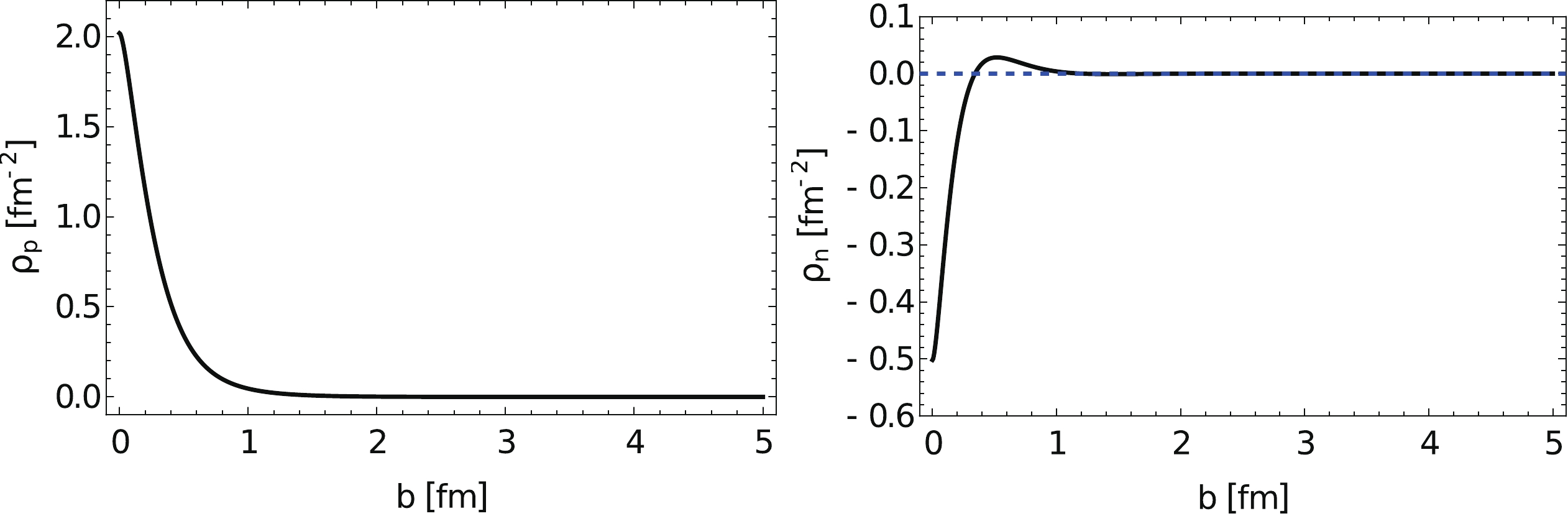
Figure 1. Transverse charge density of a proton (left) and neutron (right) in the charge-profile model.
Based on the transverse charge density, we can obtain the three-dimensional charge profile of the proton and neutron after inverted convolution using a spherical symmetry approximation, as shown in Fig. 2
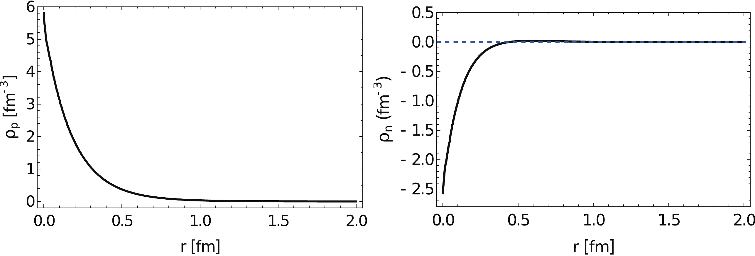
Figure 2. Three-dimensional charge profile of a proton (left) and neutron (right) in the charge-profile model.
-
With inner charge distribution models, we can investigate the space distribution of a field produced by a single nucleon by replacing the sum in Eq. (4) as an integration. For a single proton with 100 GeV, which corresponds with RHIC energies, traveling along the
$ +z $ direction, we set the time when the proton travels through$ (0,0,0) $ as$ t=0 $ fm, and then we calculate the space distribution of field at this time.With the three-dimensional charge-profile model, the results are shown in Fig. 3. Since this single proton travels with an ultra-relativistic speed, the space distribution of field is Lorentz contracted with a factor
$ \gamma = E/m $ . Therefore, we show our results on$ x-y $ plane with four different z locations. In the first panel of Fig. 3, the$ x-y $ distribution of$ B_y $ at$ z=0 $ is shown. We can observe that the magnetic field at the central location$ r=(0,0,0) $ , only the center of this single proton, is not divergent but is 0 exactly. While we increase the value of z, the strength of$ B_y $ decreases. As shown in Fig. 3(d), the strength of$ B_y $ at$ z=10/\gamma $ fm is about three orders smaller than that at$ z=0 $ .
Figure 3. (color online) Space distribution of magnetic field
$B_y$ on the$x-y$ plane with$z=0$ in Fig. 3(a),$z=1/\gamma$ (fm) in Fig. 3(b),$z=5/\gamma$ (fm) in Fig. 3(c), and$z=10/\gamma$ (fm) in Fig. 3(d) produced by a single proton with 100 GeV traveling through the$+z$ direction, calculated within the Charge-Profile model.Additionally, we checked the strength of
$ B_y $ using the point-like model. The corresponding results are shown inFig. 4. In this calculation, we have abandoned the result at$ r= $ (0, 0, 0) to eliminate divergence. We observe that the strength of$ B_y $ in the point-like model is significantly larger than that in the charge-profile model at small values of z, while the strength of$ B_y $ in the two models are similar at large z. These calculations indicate that the results within the point-like model can implement a much larger fluctuation compared with the charge-profile model. For small collision systems, because only a few nucleons contribute significantly to the magnetic field, this fluctuation will introduce many complications. Moreover, this fluctuation results only from the numerical calculation based on an unnecessary simplification. Hence, the physical charge-profile model has been introduced to calculate the electromagnetic field in this work.
Figure 4. (color online) Space distribution of the magnetic field
$B_y $ on$x-y$ plane with$z=0$ in Fig. 4(a),$z=1/\gamma$ (fm) in Fig. 4(b),$z=5/\gamma$ (fm) in Fig. 4(c), and$z=10/\gamma$ (fm) in Fig. 4(d) produced by a single proton with 100 GeV traveling through the$+z$ direction, calculated within the point-like model.In the point-like and hard-sphere models, the neutron cannot contribute to the electromagnetic field because of its neutral charge. However, as shown in Fig. 2, the neutron also has a charge profile. Therefore, the neutron can also contribute to electromagnetic field in principle. As shown in Fig. 5, the space distribution of
$ B_y $ is calculated within the charge-profile model for the neutron. The strength of field is finite and significantly smaller than the proton at a small z location, while it decreases rapidly to 0 at a large z location. This is reasonable since the neutron is charge neutral if it is measured from far away regardless of its charge distribution.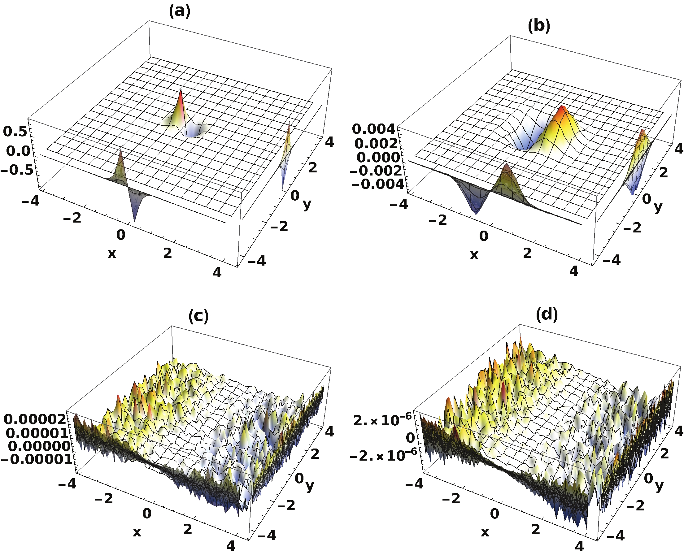
Figure 5. (color online) Space distribution of magnetic field
$B_y$ on the$x-y$ plane with$z=0$ in Fig. 5(a),$z=1/\gamma$ (fm) in Fig. 5(b),$z=5/\gamma$ (fm) in Fig. 5(c), and$z=10/\gamma$ (fm) in Fig. 5(d) produced by a single neutron with 100 GeV traveling through the$+z$ direction, calculated within the charge-profile model. -
In this section, we focus on the electric and magnetic filed produced in a high-energy small collision system
$ p+A $ . The collision geometry in our calculation is shown in Fig. 6, where b is the impact parameter, which is the distance between the centers of two nuclei. In our framework, the single proton p is treated as a projectile traveling along the$ +z $ direction, while the heavy ion A is treated as target traveling along the$ -z $ direction. We set the z coordination passing through the center of b and place the projectile at$ x=b/2 $ and the target at$ x=-b/2 $ .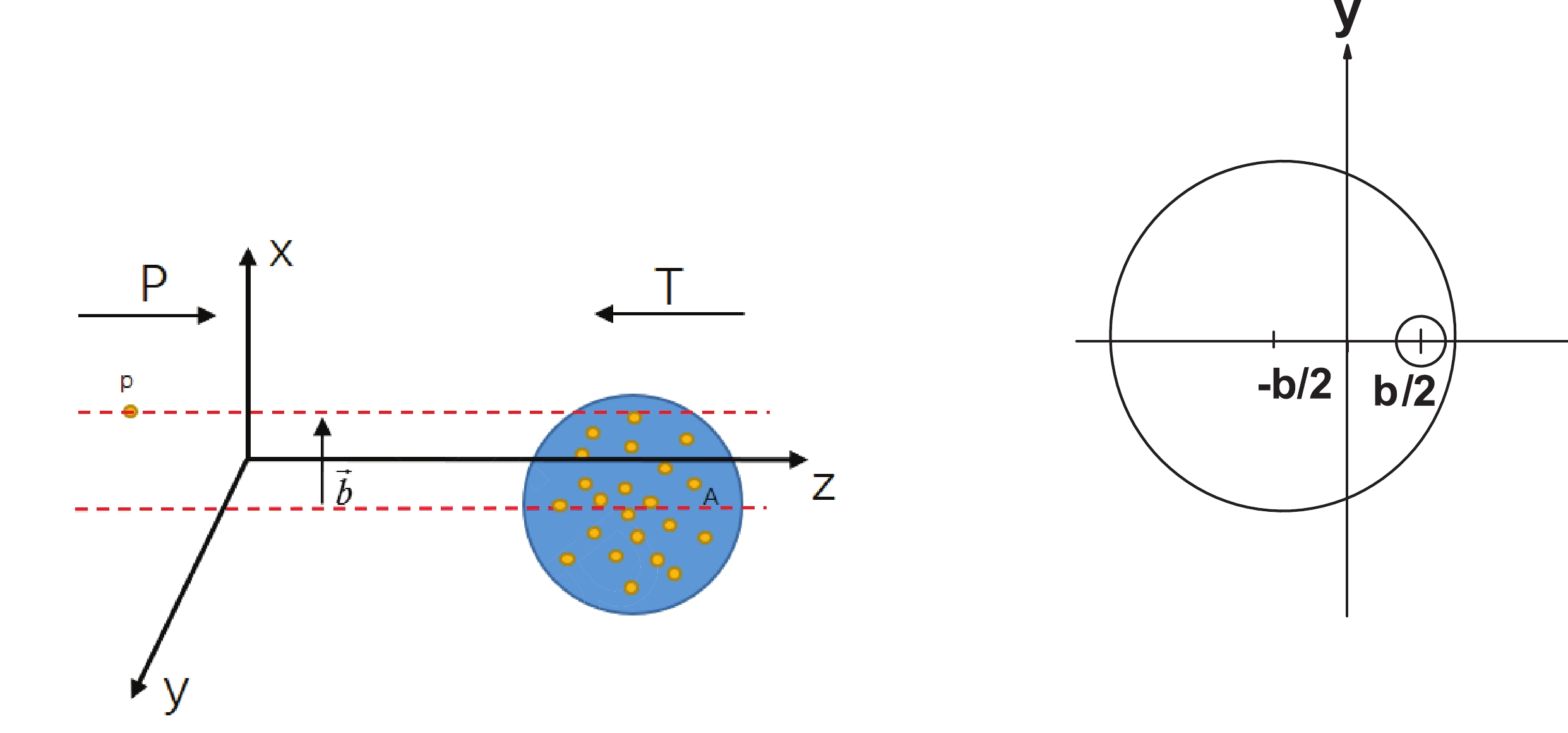
Figure 6. (color online) Geometry of a small collision system
$p+A$ .Inside the heavy ion, the position of each nucleon is sampled according to the Woods-Saxon distribution:
$ \rho_{\rm WS}(r)=\frac{\rho_0}{1+\exp[(r-R)/a]}, $

(7) where
$ \rho_0 $ =0.17 fm$ ^{-3} $ ,$ a=0.535 $ fm, and R is the radius of the incoming heavy ion. To consider the nucleon repulsive core, a minimum distance between two nucleons in a nucleus is set as 0.4 fm. subsequently, the number of participants in each event can be determined using the Monte-Carlo Glauber model.For a charge density in the nucleon of
$ \rho_n $ and nucleon distribution in the nucleus of$\rho_{\rm WS}$ , we can obtain the charge density in the nucleus using convolution, as in Eq. (8). The convotuion results for Au with$ R=6.5 $ fm are shown in Fig. 7, where the red solid curve is obtained using the charge-profile model, and the blue dashed curve is obtained using the hard-sphere model. For the point-like model, this convolutions is simply the Woods-Saxon distribution itself, shown as a black dotted curve. We can observethat the Woods-Saxon charge density distribution in the nucleus can be well reproduced with all three nucleon charge density models.
Figure 7. (color online) Charge density in the nucleus from the convolution of the Woods-Saxon nucleon distribution with three charge densities in a nucleon for Au with
$R=6.5$ fm.$ \rho_A({\boldsymbol{r}}) = \int \rho_{\boldsymbol{n}}({\boldsymbol{r}}-{\boldsymbol{r_n}}) \rho_{\rm{WS}}({\boldsymbol{r_n}}) {\rm{d}}{\boldsymbol{r_n}}\, . $

(8) -
To understand and analyze theoretical uncertainties, we calculate
$ \langle {{E_x}}\rangle $ ,$ \langle|{{B_x}}|\rangle $ ,$ \langle-{{B_y}}\rangle $ , and$ \langle|{{B_y}}|\rangle $ using the point-like, hard-sphere, and charge-profile models based on our available results of fields produced b ya single nucleon in Section III. Here, the angle bracket denotes the event average. All results shown below are the strength of fields at location${\boldsymbol{r_c}}$ which is the center of mass of all participants.In our calculation using the charge-profile model, a distance cut of |r|=4 fm is used for the charge profile of the proton and neutron. This means that if the distance between the field point and retarded source point of nucleon is less than 4 fm, we calculate the fields using its charge profile, while if the distance is larger than 4 fm, we switch to the point-like modle to calculate the field strengths. Our results show that the difference of EM field strength between the two models at this large distance is negligible. We can observe this when we compare Fig. 3 and Fig. 4. Therefore, in principle, our calculation framework does not include the distance cut-off.
-
First, in Fig. 8, we show the impact parameter dependence of the strength of fields produced within the point-like model at RHIC energies. After averaging over
$ 10^6 $ events, the value of$ E_x $ and$ B_y $ are shown (red curves in Fig. 8(a) and Fig. 8(b) still with large fluctuation, as expected. After checking contributions from participant nucleons and spectator nucleons, we observe that this large fluctuation results from the participants.
Figure 8. (color online) Electromagnetic fields at t=0 and
${\boldsymbol{r}}={\boldsymbol{r_c}}$ as a function of the impact parameter b with the point-like model.In a small collision system
$ p+A $ , there are only a few participants in each event owing to the small size of the single projectile proton. Therefore, these participants are all near the observation point${\boldsymbol{r_c}}$ . The contribution from each participant to fields may have a large strength, as shown in Fig. 4. However, because the position of each nucleon in the nucleus is random, the orientation of this field contributed from each participant is almost azimuthally random. Thus, the total field summed over these participants can remain a large strength but azimuthally random. This is the reason for large fluctuations observed within the point-like model.To obtain the strength of the fluctuation, we also calculate the impact parameter dependence of
$ |B_x| $ and$ |B_y| $ shown in Fig. 8(c) and Fig. 8(d). As these two panels show, the averaged fluctuations of fields are very large, which is almost 80 times larger than fields strength in Au+Au collisions at RHIC energies [5].With the hard-shpere model, the impact parameter dependence of fields are shown in Fig. 9. The curves in Fig. 9 are significantly smoother than those in Fig. 8. As shown in Fig. 9(a) and Fig. 9(b), the fluctuations are also significantly smaller than those of the point-like model.

Figure 9. (color online) Electromagnetic fields at t=0 and
${\boldsymbol{r}}={\boldsymbol{r_c}}$ as functions of the impact parameterb in the hard-sphere model. As shown in Fig. 9(b), the total magnetic field
$ B_y $ is contributed primarily from spectators. The strength of the total$ B_y $ and the strength from spectators both increases with the impact parameter and have maximal values at$ b \approx 6.5 $ fm. As shown in Fig. 9(a), the contribution from the participants to$ E_x $ is negative in the range of impact parameter b between 2 and 8 fm. This is simply because of the single projectile proton collisions on the periphery of the target nucleus in this range of b. Therefore, the center of mass${\boldsymbol{r_c}}$ is the approximate geometric center of all participants in each event, and the single projectile proton prefers locating on the$ +x $ side of geometry center, as shown in Fig. 10. After averaging over many events, the contributions from the target participants to$ E_x $ will offset with each other, but the contribution from the single projectile proton will remain along the$ -x $ direction.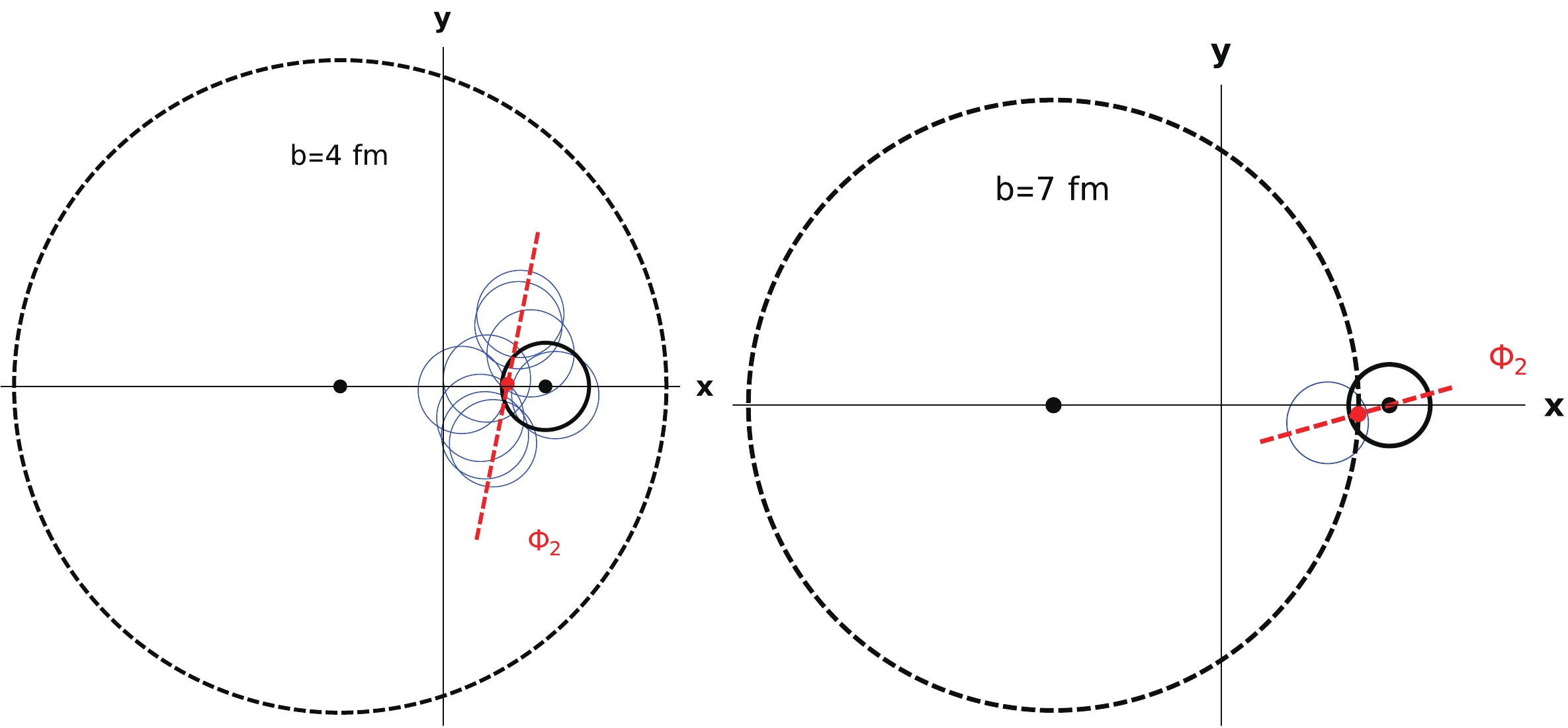
Figure 10. (color online) Examples of participant distributions in one event for
$b=4$ fm (left panel), and$b=7$ fm (right panel). The red point is the center of mass${\boldsymbol{r_c}}$ , and the red line indicates$\Phi_2$ . The blue circles are participants from thtarget nucleus, while the black circle is the single projectile proton.Fig. 11 shows the results of impact parameter dependence of fields calculated using the charge-profile model. Since the three-dimensional charge densities are obtained from electromagnetic form factors measured in experiments [33, 34], these results are more physical than those with the hard-sphere model.
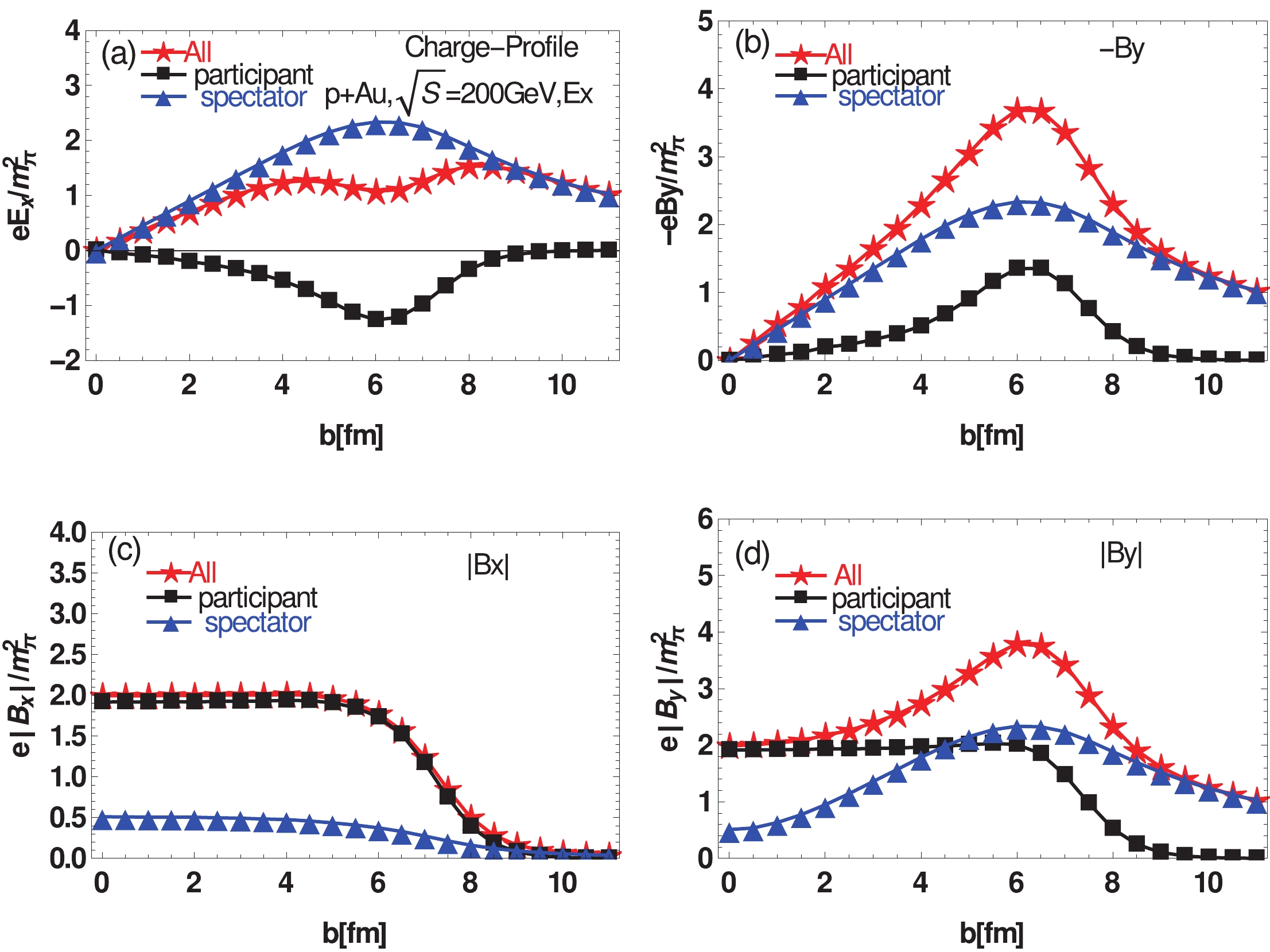
Figure 11. (color online) Electromagnetic fields at t=0 and
${\boldsymbol{r}}={\boldsymbol{r_c}}$ as functions of the impact parameter b with the charge-orofile model.Firstly, let us observe the fluctuations with the charge-profile model. As shown in Fig. 11(c) and Fig. 11(d), the fluctuation of fields from spectators are almost identical with those in the hard-sphere model. This means that the contributions from spectators are not sensitive to the detail of the inner charge distribution of the nucleon. This is because spectators are far from
$ {\boldsymbol{r_c}} $ , and the discrepancy of the inner charge density details cannot be observed clearly. In contrast, since all participants are near$ {\boldsymbol{r_c}} $ , their contributions are not negligible; thus, the fluctuations from participants are considerably different from those in the hard-sphere model.For the strength of electric fields
$ E_x $ shown in Fig. 11(a), the contribution from all participants is still negative, similar to that in the hard-sphere model, since the contribution from single projectile proton remains along the$ -x $ direction. Its negative strength is so large that a significant depression occurs to the total$ E_x $ at$ b \approx 6 $ fm.In Fig. 11(b), although strength of
$ B_y $ contributed from spectators is similar with that of the hard-sphere model, the contribution from participants is significantly larger. In peripheral collisions, in particular, contributions from participants are of the same order as spectators. This is the main difference compared with heavy-ion$ A+A $ collision systems. Since the orientation of the event plane is determined only by participants, this large contribution of the participants to$ B_y $ may induce a significant azimuthal correlation between the event plane$ \Phi_2 $ and magnetic field$ \Phi_B $ .Compared with the magnetic strength of
$ B_y $ in Ref. [30], our result within the charge-profile model is about half. Considering the very small size of overlapping area in small collision system, any discrepency in the inner charge density of nucleion can result in a significant difference in field strengths. We arrive at this same conclusion when we compare Fig. 3(a) and Fig. 4(a). Thus, beyond the hard-sphere model, we also implement the realistic charge-profile model in our calculation. -
As mentioned earlier,
$ \Delta\gamma\propto B^2\cdot\cos2(\Phi_B-\Phi_2) $ , where$ \Phi_B $ is the angle of the magnetic field${\boldsymbol{B}}$ direction. In this section, we focus on the second harmonic participant plane$ \Phi_2 $ as it is the most prominent anisotropy from bot geometry and fluctuations. The corresponding initial event plane angles are given by:$ \Phi_{{n}}=\frac{1}{{{n}}}\arctan\frac{<{{r}}^{{n}}\sin({{n}}\phi)>}{<{{r}}^{{n}}\cos({{n}}\phi)>} $

(9) where r is the distance of the participant particles from
${\boldsymbol{r_c}}$ , ϕ is the angle between the x direction and the direction of r [35]. We define$ \Phi_2 $ as the long axis direction of the ellipse, as shown in Fig. 10; our definition of the reaction plane in this work differs from experiments.Our calculations in this subsection are all within the charge-profile model to obtain a physical understanding of the azimuthal correlation between
$ \Phi_B $ and$ \Phi_2 $ . First, we provide the distribution of the discrepancy$ \Phi_B - \Phi_2 $ in Fig. 12. We can observe a strong negative correlation between$ \Phi_B $ and$ \Phi_2 $ at large b; this is because only one nucleon in the target nucleus can be hit by single projectile proton in this very peripheral collision, as illustrated in right panel of Fig. 10. Therefore, the direction of$ \Phi_2 $ (the long axis of ellipse) is preferred near the x direction, which is perpendicular to the direction of the magnetic field.
Figure 12. Normalized distribution of the discrepency between
$\Phi_B$ and$\Phi_2$ at t=0 and${\boldsymbol{r}}={\boldsymbol{r_c}}$ with three different impact parameters b=0 fm, b=5 fm, and b=7 fm, respectively, within the charge-profile model.At small and middle values of b, there is a slight but not negligible correlation between
$ \Phi_B $ and$ \Phi_2 $ , even at$ b=0 $ fm, as shown in the first panel on Fig. 12. This phenomenon can also be explained using the left panel in Fig. 10. In each event, the contribution to fields from the single projectile proton is very large compared with the target participants since$ {\boldsymbol{r_c}} $ is very close to it. While the location of this single projectile proton prefers the$ +x $ side of$ {\boldsymbol{r_c}} $ in the event, its contribution to$ B_y $ prefers the$ -y $ direction in each event. In contrast, owing to nuclear geometry, the target participants overlap as an approximate ellipse with their long axis along the y direction.This correlation between
$ \Phi_B $ and$ \Phi_2 $ can also be observed in the azimuthal correlation factor$ \cos2(\Phi_B-\Phi_2) $ , shown in left panel of Fig. 13. We observe that the value of this correlation factor is very small but not vanished at small and middle ranges of the impact parameter b. In the large b range, the azimuthal correlation shown in the lower panel of Fig. 12 appears again. This result corresponds with that in Ref. [29].
Figure 13. The left panel shows the azimuthal correlations between the magnetic field plane
$\Phi_B$ and$\Phi_2$ , the two curves correspond to the participant plane (solid) and spectator plane (dashed). The right panel shows$B^2\cdot\cos2(\Phi_B-\Phi_n)$ as a function of impact parameter for$p+{\rm Au}$ at RHIC energies.Since the CME induced charge separation effect is described as
$ \Delta\gamma\propto B^2\cdot\cos2(\Phi_B-\Phi_2) $ , we show this$ B^2 $ evolved azimuthal correlation in the right panel of Fig. 13. Owing to the large fluctuation in the strength of the magnetic field (Fig. 11(d)), the slight remaining azimuthal correlation can produce a finite$ \Delta\gamma $ signal owing to the CME effect.We have also checked the azimuthal correlation between the magnetic direction
$ \phi_B $ and spectator plane$ \phi_{2s} $ . The distributions of the discrepancy$ \Phi_B - \Phi_{2s} $ are shown in Fig. 14. These results show that the azimuthal coupling between$ \phi_B $ and spectator plane$ \phi_{2s} $ at small and middle values of b almost vanishes, which is in contrast to the participant plane. This decoupling of$ \phi_B $ and$ \phi_{2s} $ can also be observed on the left panel of Fig. 13.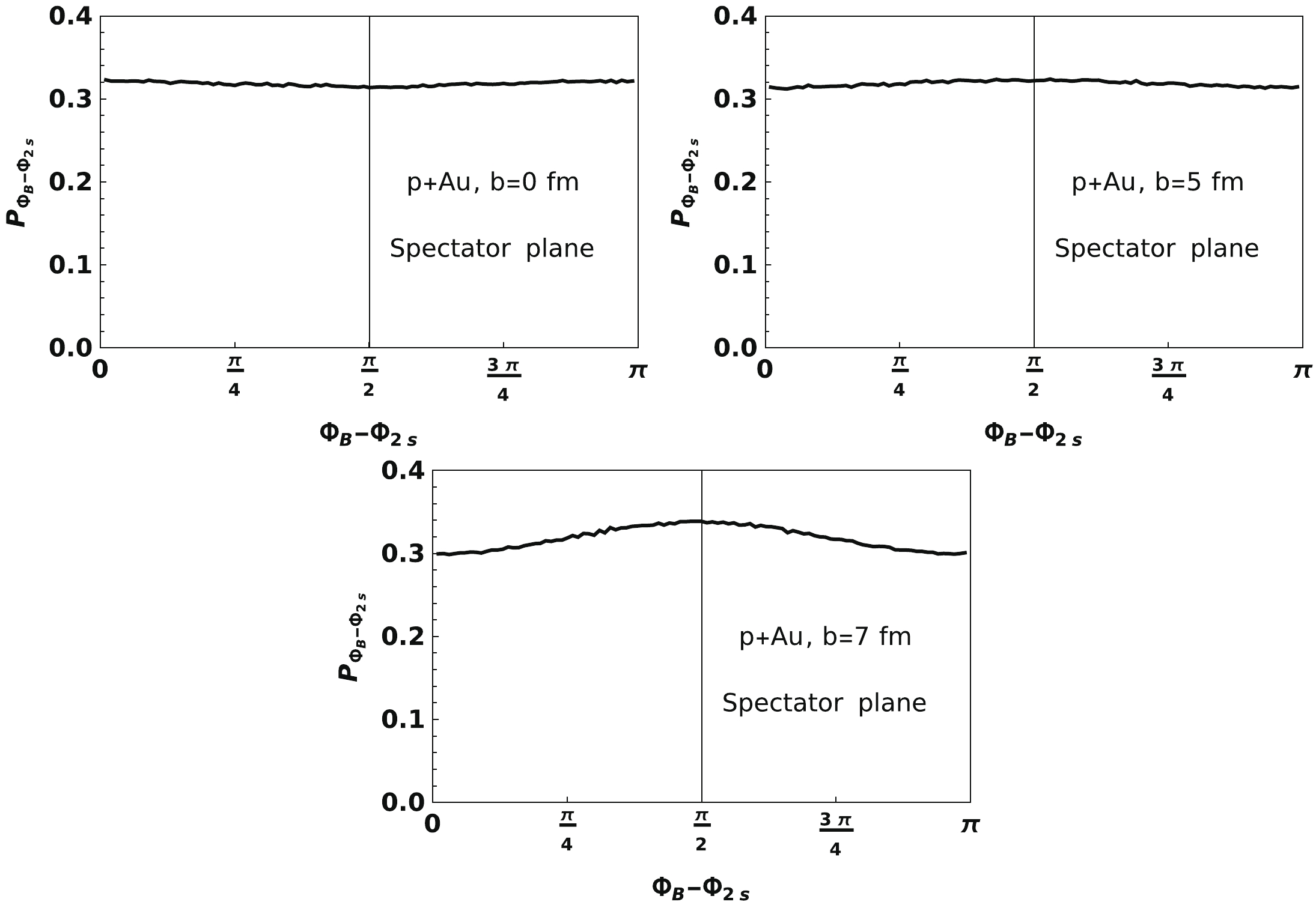
Figure 14. Normalized distribution of the discrepancy between
$\Phi_B$ and$\Phi_{2s}$ at t=0 and$\boldsymbol{r}=\boldsymbol{r}_c$ with three different impact parameters b=0 fm, b=5 fm, and b=7 fm, respectively, within the charge-profile model.This calculation can be easily extended to LHC energies. We give corresponding results in Fig. 15. The result of azimuthal correlation
$ \cos2(\Phi_B-\Phi_2) $ at LHC energies is similar with those at RHIC energies. Owing to the significant fluctuation of the strength of magnetic field, the$ B^2 $ evolved azimuthal correlation$ B^2\cdot\cos2(\Phi_B-\Phi_n) $ at LHC energies is three orders larger than those at RHIC energies.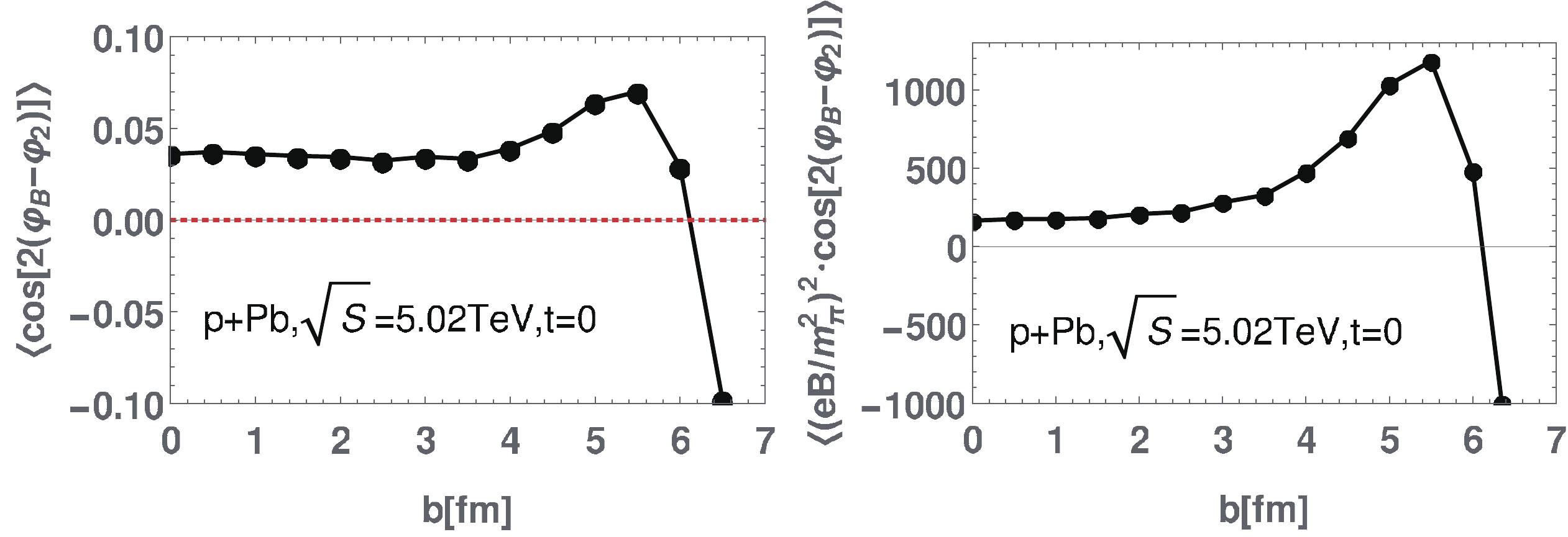
Figure 15. (color online) The left panel shows the azimuthal correlations between magnetic field plane
$\Phi_B$ and$\Phi_2$ , while the right panel shows$B^2\cdot\cos2(\Phi_B-\Phi_n)$ as a function of impact parameter for$p+{\rm Pb}$ at LHC energies.Although all of our results are shown on only one special spatial point
${\boldsymbol{r_c}}$ , the discovery of the azimuthal correlation at this special point is sufficiently important, because the possible CP violation in QGPs is not a global but a local effect. This strong azimuthal correlation between$ \Phi_B $ and$ \Phi_2 $ implies that the CME signals may be observed in the small system and may partly explain the observed$ \Delta\gamma $ experimental data [19, 31]. -
The contribution of the CME to the charge separation effect is related not only with the strength of magnetic field, but also with the angle between direction of magnetic field
$ \Phi_B $ and reaction plane$ \Phi_2 $ . In the heavy-ion small collision systems with p+A or d+A collisions, the direction of the magnetic field was initially believed to be determined primarily by the distribution of spectators, while the direction of reaction plane was computed from the space distribution of participants. Owing to the decoupling of the angular correlation between the reaction plan and direction of magnetic field, this charge separation effect should be vanished. However, experimental data indciates a considerably different result compared with theory predictions.Employing a physical charge-profile model to describe the inner charge distribution of a proton and a neutron, we systematicallycalculate the property of electromagnetic field produced in a small system, at both RHIC and LHC energies, including its dependence on the impact parameter b. In particular, we carefully study the azimuthal correlation between
$ \Phi_B $ and$ \Phi_2 $ .In contrast with previous expectations, our results show a significant angular correlation between them. This correlation results primarily from the very close distance between the location of the single projectile proton and location of the center of mass
${\boldsymbol{r_c}}$ of the hot medium produced in a small collision system. The contribution of a single projectile proton to the magnetic field is the main source after averaging over all participants. Therefore, the strong angular distribution priority of this single projectile proton can contribute significantly to the angular correlation of$ \Phi_B $ and$ \Phi_2 $ .This discovery breaks through previous concepts about the magnetic filed produced in small collision systems. It can aid us in clarifying the contribution of the CME to the observation in small-system-collision experiments. We should also point out that our resuts here are only at
$ t=0 $ fm. Whether the CME can be observed in small systems depends on how long the magnetic field lasts and the effects of the final state interactions on the initial CME signal in small systems.In our next study, a more realistic nuclear collision model, such as the HIJING or AMPT model, will be implemented with our framework of the charge-profile model. We will check whether this azimuthal correlation between
$ \Phi_B $ and$ \Phi_2 $ can be kept or not in the time evolution of collision systems. -
We thank Xu-Guang Huang for very helpful discussions.
Electromagnetic field produced in high-energy small collision systems within charge density models of nucleons
- Received Date: 2022-02-28
- Available Online: 2022-08-15
Abstract: Recent experiments show that


 DownLoad: