


 Abstract
 HTML
HTML Reference
 Related
 PDF
PDF


-
Since the concept of black hole was proposed, people have been trying to find this mysterious physical object in the universe. Recently, the first image of the supermassive black hole at the center of M87
$^* $ galaxy, which was captured by the Event Horizon Telescope (EHT) Collaboration, is a strong proof of the existence of black holes [1–6]. A bright ring appears around a dark area in the image, where the dark area in the center is called the black hole shadow and the bright area is the photon sphere. It is commonly known that the strong gravity of black hole deflects light and forms the black hole shadow, which was also known as the gravitational lensing effect [7]. With the deepening of the study of black holes, people pay more attention to the observation of black hole shadows, because this will bring new insights and development to the study of black holes. There is a lot of research into black hole shadows under different gravitational backgrounds, such as finding extra dimensions through the black hole shadow characteristics, the gravitational lensing effect, the shape and size of the shadow for a rotating or non-rotating black hole, constraining the relevant parameters by shadow features, and so on [8–43].In our universe, real astrophysical black holes in galaxies are surrounded by a large amount of high-energy radiation material, which makes it possible to indirectly observe the black hole [44]. The accretion flow around a black hole is usually not spherically symmetric, but the simplified ideal spherical model can provide strong support for the characteristics of black hole observation. It is generally accepted that the shape of the black hole shadow has a standard circular geometry in a static spherically symmetric spacetime [45]. In Ref. [46], Bardeen pointed out that the radius of shadow for a Schwarzschild black hole is
$ r_s=3 M $ , where M is the mass of black hole. Bardeen also mentioned that the shape of the shadow for a rotating black hole is closely related to angular momentum. In 1979, a simulated image of a black hole was shown for the first time, in which a black hole surrounded by an optically thin disk was considered [47]. For a model in which the black hole is surrounded rather by an optically thin spherical accretion, it has been found that the shadow is dependent on the geometric characteristics of the spacetime, and has nothing to do with the details of the accretion process [48]. However, the observed luminosity is affected by the accretion flow model [49–53]. When an optically and geometrically thin disk accretion is located on the equatorial plane of the black hole, the observational peculiarities of the black hole shadow observed by a distant observer have been studied in Ref. [54]. Gralla et al. classified the trajectories of light rays near the black hole, whereby dividing the rings outside the shadow area into direct, photon ring, and lensing ring, and proposed that the observed intensity is dominated by the direct case. Furthermore, they also found that the size of the dark central region depends on the specific emission model of accretion flow. Using different accretion flow models, there is a series of interesting observable features about the shadow and rings of the black hole in other gravitational spacetime backgrounds; see Refs. [55–65].Most often, the black hole has a singularity inside the horizon. However, in Ref. [66], a model of a black hole with regular non-singular geometry was proposed by Bardeen. In this system, an energy–momentum tensor is introduced, which is interpreted as the gravitational field of a nonlinear magnetic monopole charge. Since then, the physical properties of the Bardeen black hole has aroused people's interest, and involve a wide range of quasinormal modes, energy distribution, radiation, thermodynamic behavior and so on [67–80]. Indeed, the study of black hole shadows can explore the basic physical properties of the spacetime. Therefore, it is necessary to study the shadow and observed characteristics in the context of the Bardeen spacetime. In this paper, we focus on the shadow and observed luminosity of a Bardeen black hole surrounded by various accretion models, namely the static model, infalling spherical accretion and optically thin disk accretion, which were regarded as the only background light source. By comparing the results in this work with the Schwarzschild spacetime, we can study the influence of the magnetic monopole charge on the shadow and observed characteristics, due to the charge parameter which has a remarkable role in the Bardeen spacetime. Therefore, this may provide a feasible method to distinguish the Bardeen spacetime from the Schwarzschild spacetime.
The paper is organized as follows. In section II, we study the associated trajectories of light rays near a Bardeen black hole, as well as the radius of the photon sphere and the black hole shadow when the state parameters are changed. In section III, we analyze the shadow image and luminosity of the black hole surrounded by the different spherical accretion models. In section IV, we consider thin disk emission near the black hole, and compare the observed appearance with different emission profiles. Finally, we discussed our results and conclusions in section V. In this paper, we use the units
$ G = c = 1 $ . -
We would like to consider the spherically symmetric spacetime, with the metric of the Bardeen regular black hole as follows [66],
$ {\rm d} s^2=-A(r) {\rm d} t^2 +B (r) {\rm d} r^2 +C (r) \left({{\rm d}\theta }^2+ \sin ^2 \theta {{\rm d} \varphi }^2 \right), $

(1) with
$ A(r)=1-\frac{2 M r^2}{\left(g^2+r^2\right)^{3/2}},\quad B(r)=\frac{1}{A(r)}, \quad C (r)=r^2, $

(2) in which M is the mass of the black hole and g is the magnetic charge of a self-gravitating magnetic field described by a nonlinear electrodynamic source. Note that the spacetime structure could recover to the Schwarzschild spacetime in the case where
$ g\rightarrow0 $ . As mentioned in Ref. [67], the metric function can be approximated as$ A (r)\sim 1-\frac{2 M}{r}+\frac{3 g^2 M}{r^3}+{{\cal{O}}}\left(\frac{1}{r^5}\right). $

(3) It is clear that the form of the above equation is different from the Reissner–Nordström spacetime. The horizon of the Bardeen black hole can be obtained by
$ A (r)=0, $

(4) where the largest positive root is the event horizon of the black hole. It is worth noting that the solution (1) is parameterized by the mass parameter M and magnetic charge g, so changing the specific magnetic charge
$ g/M $ will directly affect the geometry of the spacetime. When the specific magnetic charge$ g/M<\dfrac{4\surd3}{9} $ , which is an important threshold for the existence of the event horizon, there is one unstable null circular geodesic located out of the event horizon. For the case$ g/M > \dfrac{4\surd3}{9} $ , there is no horizon; we do not consider this case in this paper [81]. A light ray passing in the vicinity of a massive object is deflected due to the interaction between the light and the gravitational field of the massive object. We can use the Euler–Lagrange equation to investigate the motion of photons around the Bardeen black hole, which reads as$ \frac{{\rm d}}{{\rm d}\lambda }\left(\frac{\partial {\cal{L}}}{\partial \dot{x}^{\mu }}\right)=\frac{\partial {\cal{L}}}{\partial x^{\mu }}, $

(5) where λ and
$ \dot{x}^{\mu } $ are the affine parameter and four-velocity of the photon, respectively. For the metric function (1), the Lagrangian$ {\cal{L}} $ can be expressed as$ {\cal{L}}=\frac{1}{2} g_{\mu \nu } \dot{x}^{\mu } \dot{x}^{\nu }=\frac{1}{2} \left(-A (r) \dot{t}^2+B (r) \dot{r}^2+C (r) \left(\dot{\theta} ^2+ \sin\theta ^2 \varphi ^2\right)\right). $

(6) In the spherically symmetric spacetime, we discuss the motion of photons confined to the equatorial plane of a black hole [10, 45, 82], with the restrictive conditions
$ \theta =\dfrac{\pi }{2} $ and$ \dot{\theta} =0 $ . As the t and θ coordinates can not explicitly determine the coefficient of the metric equation, there are two conserved quantities E and L, representing energy and angular momentum, respectively. That is$ E=-\frac{\partial {\cal{S}}}{\partial \dot{t}}=A (r) \dot{t},\quad L=\frac{\partial {\cal{S}}}{\partial \dot{\varphi} }=r^2 \dot{\varphi}. $

(7) For the null geodesic
$ g_{\mu \nu } \dot{x}^{\mu } \dot{x}^{\nu }=0 $ , we can obtain the orbit equation$ \dot{r}^2+V_{\rm eff}=\frac{1}{b^2}, $

(8) in which
$V_{\rm eff}$ is the effective potential, which is given by$ V_{\rm eff}=\frac{1}{r^2} \left(1-\frac{2 M r^2}{\left(g^2+r^2\right)^{3/2}}\right), $

(9) Moreover, b is called the impact parameter, which is the ratio of angular momentum to energy, i.e.,
$ b = L/E= \dfrac{r^2 \dot{\varphi}}{A (r) \dot{t}} $ . In the spacetime (1), there exists a critical impact curve with radius$ b_p $ , for which the light along this curve will asymptotically approach a bound photon orbit. For the position of the photon sphere, the effective potential should follow the condition$ \dot{r}=0 $ and$ \ddot{r}=0 $ , which means [50]$ V_{\rm eff}=\frac{1}{b ^2},\quad 2 V'_{\rm eff}=0. $

(10) From Eq. (10), one can find the relation between the photon sphere radius
$ r_p $ and critical impact parameter$ b_p $ $ r_p{}^2-b_p^2 A(r)=0,\quad 2 b_p^2 A(r)^2-r_p{}^3 A'(r)=0. $

(11) Indeed, the inner region of the critical curve is the shadow region of the black hole, that is, the critical impact parameter
$ b_p $ is the shadow radius that can be seen by a distant observer ($ r_o\rightarrow \infty $ ). In the spacetime (1), changing the parameters M and g will directly affect the geometric structure. Hence, for the different values of the specific magnetic charge$ g/M $ , we show the different numerical results for the photon sphere radius$ r_p $ , shadow radius$ b_p $ and event horizon$ r_h $ , as listed in Table 1. In order to reflect the difference between the Bardeen and Schwarzschild spacetime, we take the value of$ b_p $ of the Schwarzschild case ($ g\rightarrow 0 $ ), which corresponds to the value in Table 1, i.e., the shadow radius in these two spacetimes is equal, and show the corresponding physical quantities of Schwarzschild black hole in Table 2.$g/M=0$ 

$g/M=0.1$ 

$g/M=0.2$ 

$g/M=0.475$ 

$g/M=0.6$ 

$g/M=0.7$ 

$g/M=0.75$ 

$b_{p}$ 

$3 \surd 3$ 

5.18747 5.16108 4.98508 4.83975 4.67719 4.57212 $r_{p}$ 

3 2.99164 2.96617 2.7937 2.64674 2.47495 2.35745 $r_{h}$ 

2 1.99247 1.96946 1.80981 1.66546 1.47436 1.29904 Table 1. Values of relevant physical quantities in the Bardeen spacetime under different values of specific magnetic charge
$g/M$ , in which$M=1$ .$M=1$ 

$M=0.99833$ 

$M=0.99325$ 

$M=0.95938$ 

$M=0.93141$ 

$M=0.90013$ 

$M=0.87991$ 

$b_{p}$ 

$3 \surd 3$ 

5.18747 5.16108 4.98508 4.83975 4.67719 4.57212 $r_{p}$ 

3 2.99499 2.97975 2.87814 2.79423 2.70038 2.63972 $r_{h}$ 

2 1.99666 1.9865 1.91876 1.86282 1.80025 1.75981 Table 2. Values of relevant physical quantities in the Schwarzschild spacetime under different values of mass.
From Table 1, it can be found that all related physical quantities
$ r_p $ ,$ b_p $ and$ r_h $ show a decreasing trend with the increase of specific magnetic charge$ g/M $ . In the Schwarzschild spacetime ($ g = 0 $ ), the values of$ r_p $ ,$ b_p $ and$ r_h $ are larger than those of Bardeen case ($ g \neq 0 $ ). In Table 2, the shadow radius$ b_p $ of the Schwarzschild black hole is consistent with that of the Bardeen black hole, but the corresponding photon sphere and event horizon radius of the Schwarzschild black hole are slightly larger than those in the Bardeen spacetime. In other words, although the shadow radii observed in these two spacetime are equal, the observed luminosity and appearance could be different, as the geometric structure of the Schwarzschild and Bardeen spacetime are different.With the help of introducing parameter
$ u_0=1/r $ , we can rewrite the equation of motion for photons, and use it to depict the trajectory of light ray:$ {\cal{V}}(u_0)=\frac{{\rm d} u_0}{{\rm d}\varphi }=\sqrt{\frac{1}{b^2}-u_0^2 \left(1-\frac{2 M}{u_0^2 \left(g^2+\dfrac{1}{u_0^2}\right)^{3/2}}\right)}. $

(12) It is worth noting that the geometry of geodesics depends entirely on Eq. (12), which is a function of the impact parameter b. In the case of
$ b<b_p $ , the light ray is always trapped by the black hole and cannot reach infinite distance. In the case of$ b>b_p $ , the light ray will be deflected at the radial position$ u_0 $ where$ {\cal{V}}(u_0)=0 $ , and then move away from the black hole to reach infinite distance. When$ b=b_p $ , the photons are in a state of rotation around the black hole, neither falling into the black hole nor escaping. In the following sections, we further study the shadow of a black hole surrounded by various profiles of accretion flow. -
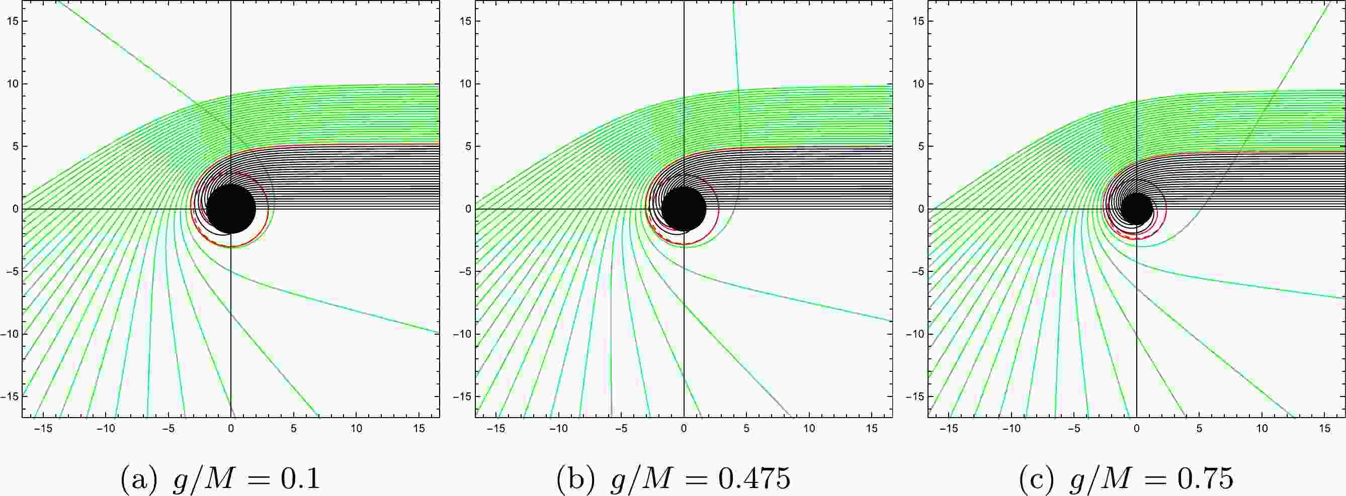
From equation (12), we find that the trajectory of a light ray changes as we change the value of specific magnetic charge
$ g/M $ and impact parameter b. Therefore, we simply describe the path of light rays under the relevant physical parameters, as shown in Fig. 1. In The red, green lines and black lines correspond to$ b=b_p $ ,$ b>b_p $ and$ b<b_p $ , respectively. When the value of specific magnetic charge$ g/M $ increases, the radius of the photon sphere$ r_p $ decreases, as well as the event horizon$ r_h $ . Furthermore, the deflection rate of light rays is different under the different values of specific magnetic charge$ g/M $ . This means that the light density obtained by distant observers is different, which naturally leads to a different observed intensity cast by the black hole shadow. When the value of$ b_p $ is equal to that in Fig. 1, the trajectory of light near the black hole in the Schwarzschild spacetime is shown in Fig. 2. We found that the light trajectories and deflections near the black hole are different from the Bardeen case, which means that the appearance of magnetic charge g will lead to different observed intensity in these two spacetimes, even though the observed shadow radii are equal.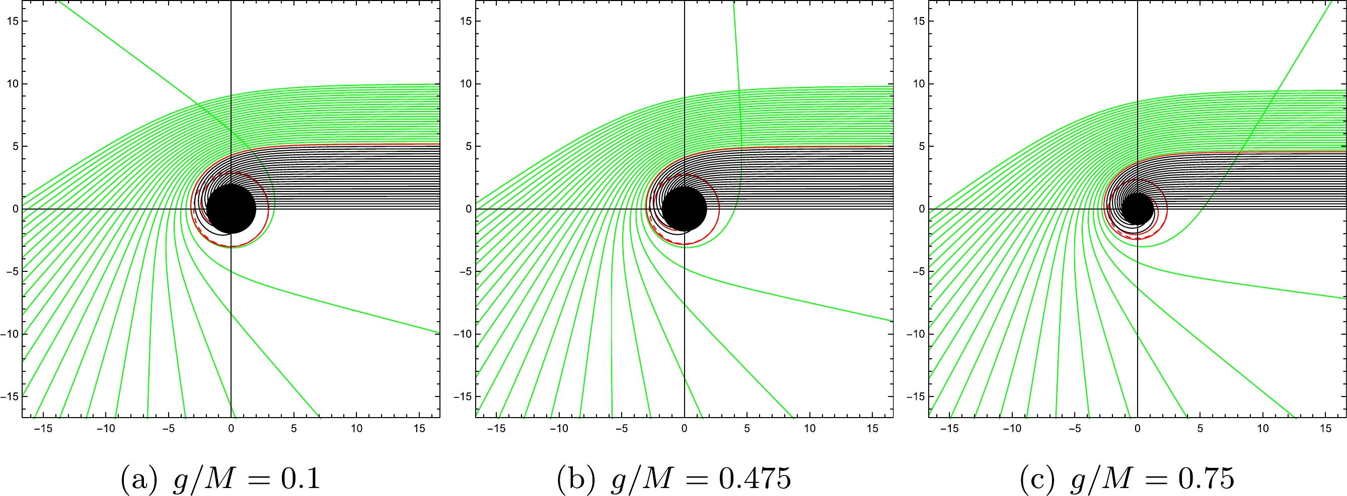
Figure 1. (color online) Trajectories of light rays for different values of specific magnetic charge
$ g/M $ in the polar coordinates$ (r, \varphi) $ , where$ M=1 $ . Here, the black hole is shown as a black disk, and the red dotted line represents the position of the photon sphere.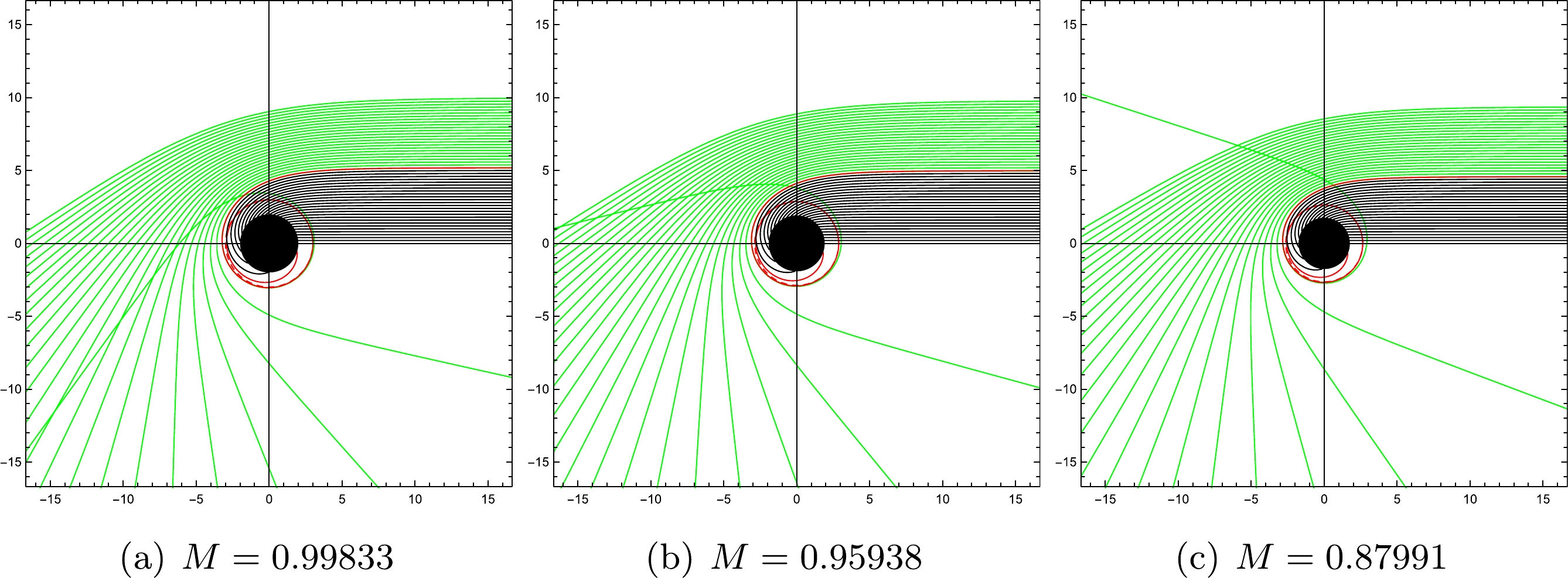
Figure 2. (color online) Trajectories of light rays for the case
$ g=0 $ (the Schwarzschild spacetime) for different values of M in polar coordinates$ (r, \varphi) $ . Here, the black hole is shown as a black disk, and the red dotted line represents the position of the photon sphere. -
For the distant observer, we want to study the observed luminosity of the black hole shadow, in which the accretion flow around the black hole is the only light source. We introduce two simple relativistic spherical accretion models, namely, static spherical accretion and infalling spherical accretion. In the background of the black hole being wrapped by static spherical accretion flow, we can integrate the specific emissivity along the photon path
$ \gamma_i $ , and so obtain the specific intensity$ {\cal{I}}_{{\rm obs}} $ for the distant observer (usually measured in ergs−1cm−2str−1Hz−1). That is [8, 50]$ {\cal{I}}_{{\rm obs}}(\nu _0)=\int _{\gamma _i}{g_s}^3 {j} (\nu _e) {\rm d} l_{{\rm prop}}, $

(13) and
$ g_s=\frac{\nu _o}{\nu _e}. $

(14) It is worth mentioning that we focus on the case where the emitter is fixed in the rest frame. In the above equation,
$ g_s $ is the redshift factor and$ \nu _e $ is the photon frequency at the emitter. In addition,$ {j} (\nu _e) $ is the emissivity per-unit volume at the emitter,${\rm d} l_{{\rm prop}}$ is the infinitesimal proper length, and$ \nu _0 $ is the observed photon frequency, respectively. In the spacetime (1), the redshift factor$ g_s=A(r)^{1/2} $ . For the specific emissivity$ {j} (\nu _e) $ , we consider that the emission is monochromatic with emission frequency$ \nu _f $ and the emission radial profile is$ 1/r^2 $ , that is,$ {j} (\nu _e)\sim\frac{\delta \left(\nu _e-\nu _f\right)}{r^2}, $

(15) where δ is the delta function. In addition, we can obtain the proper length
${\rm d}l_{{\rm prop}}$ as$ {\rm d}l_{{\rm prop}}= \sqrt{\frac{1}{A (r)}+r^2 \left(\frac{{\rm d}\varphi }{{\rm d} r}\right)^2} {\rm d} r. $

(16) Then, the expression of the observed specific intensity can be rewritten as
$ {\cal{I}}_{{\rm obs}}(\nu _o )=\int _{\gamma _i}\frac{(A (r))^{3/2}}{r^2} \sqrt{\frac{1}{A (r)}+r^2 \left(\frac{{\rm d}\varphi }{{\rm d}r}\right)^2} {\rm d}r. $

(17) In Eq. (17), the total observed intensity
${\cal{I}}_{{\rm obs}}(\nu _o )$ as a function of impact parameter b. In addition, the change of a relevant physical quantity will directly affect the specific intensity observed by a distant observer. Taking the value of specific magnetic charge$ g/M=0.1, 0.475, 0.75 $ as examples, we give the trend of observed intensity with impact parameter b for the different values of specific magnetic charge$ g/M $ in Fig. 3.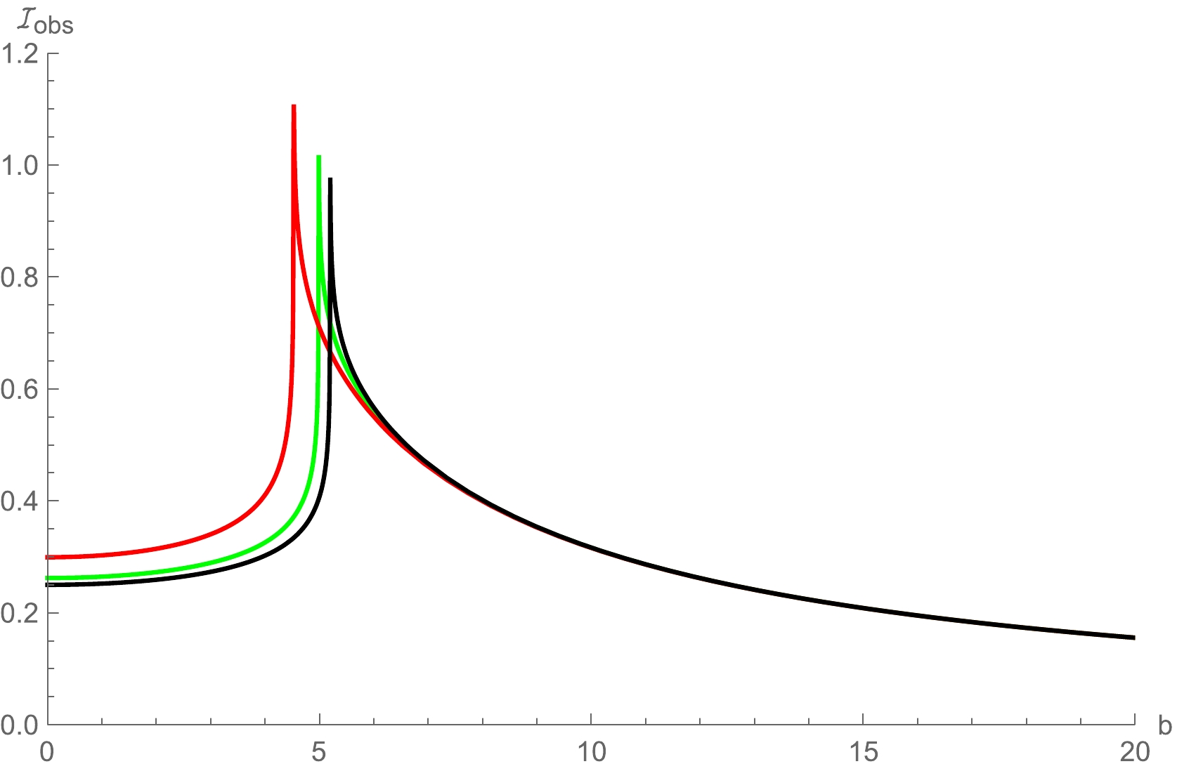
Figure 3. (color online) Observed specific intensity of the black hole surrounded by static spherical accretion flow. Here, the black, green and red lines correspond to
$ g/M=0 $ ,$ g/M=0.475 $ and$ g/M=0.75 $ , respectively, and$ M=1 $ .It is clear that the observed intensity increases slowly with the increase of b (
$ b<b_p $ ), but increases rapidly near the photon sphere ($ b=b_p $ ) until it reaches a peak at the position of the photon sphere. After that, the observed intensity decreases with the increase of b ($ b>b_p $ ) until at infinity${\cal{I}}_{{\rm obs}}(\nu _o )\rightarrow0$ . In addition, the larger the value of specific magnetic charge$ g/M $ , the stronger the specific intensity observed. For the case$ g/M =0 $ (the Schwarzschild spacetime), the peak of observed intensity is clearly smaller than when$ g/M=0.45 $ (or$ g/M=0.75 $ ). In other words, the observed intensity of the Bardeen black hole is stronger than that of the Schwarzschild spacetime, and higher values of specific magnetic charge$ g/M $ will enhance the light density, so that the observer can obtain more luminosity. The two-dimensional intensity map in celestial coordinates casted by the black hole is shown in Fig. 4.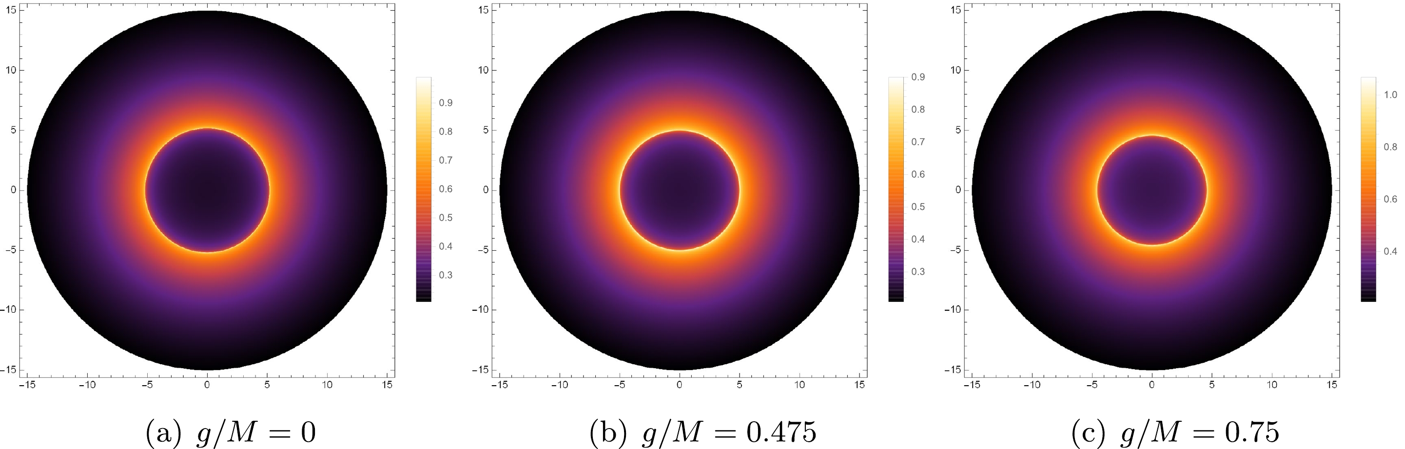
Figure 4. (color online) Image of the black hole shadow with the static spherical accretion for different values of specific magnetic charge
$ g/M $ , in which$ g/M=0 $ (left panel),$ g/M=0.475 $ (mid panel) and$ g/M=0.75 $ (right panel). Here, we take$ M=1 $ .In Fig. 4, there exists a bright ring with the strongest luminosity, which is the position of photon sphere. As a tiny fraction of the radiation can escape from the black hole, the inner region of the photon sphere is not completely black, and there is small observed luminosity near the photon sphere. Clearly, the maximum luminosity of the shadow image is enhanced with the increase of specific magnetic charge
$ g/M $ , while the size of the shadow and the radius of photon sphere is decreased. -
In the background of a black hole surrounded by infalling spherical accretion, radiating gas moves towards the black hole along the radial direction. Indeed, the infalling spherical accretion is closer to the real situation than the static spherical accretion model. Equation (17) is still suitable in the infalling accretion model, but the redshift factor is different from the static case. In the infalling accretion model, the redshift factor is related to the velocity of the accretion flow, namely
$ g_i=\frac{{\cal{K}}_{\rho } u _0^{\rho }}{{\cal{K}}_{\sigma } u _e^{\sigma }}, $

(18) and
$ {\cal{K}}^{\mu }=\dot{x}_{\mu }, $

(19) in which
$ {\cal{K}}^{\mu } $ is the four-velocity of the photon and$ u_0^{\mu }=(1,0,0,0) $ is the four-velocity of the static observer. Moreover, the four-velocity of the infalling accretion corresponds to$ u_e^{\mu } $ , which is$ u_e^t={A (r)}^{-1},\quad u_e^r=-\sqrt{\frac{1-A (r)}{A (r) B ( r)}}, \quad u_e^{\theta }=u_e^{\varphi }=0. $

(20) Here,
$ {\cal{K}}_t $ is a constant of motion. For the photon,$ {\cal{K}}_r $ can be obtained by the equation$ {\cal{K}}_{\mu } {\cal{K}}^{\mu }=0 $ , and consequently$ {\cal{K}}_t=\frac{1}{b}, \quad \frac{{\cal{K}}_r}{{\cal{K}}_t}=\pm \sqrt{B (r) \left(\frac{1}{A (r)}-\frac{b^2}{r^2}\right)}, $

(21) in which the sign
$ + $ or$ - $ corresponds to the photon approaching or going away from the black hole. Hence, the redshift factor of the infalling accretion is$ g_i=\left(u_e^t+\left(\frac{{\cal{K}}_r }{{\cal{K}}_e}\right)u_e^r \right) ^{-1}. $

(22) On the other hand, the form of the proper distance should be rewritten as
$ {\rm d} l_{\rm prop}={\cal{K}}_\mu u_e ^\mu {\rm d}\lambda=\frac{{\cal{K}}_t}{g_i |{\cal{K}}_r|} {\rm d} r. $

(23) Considering that the specific emissivity has the same form as in the equation (15), the observed flux for the distant observer in the case of infalling spherical accretion model is
$ {\cal{I}}_{{\rm obs}}({\nu^i_{o}})\propto \int _{\gamma _i}\frac{g_i^3 {\cal{K}}_t {\rm d} r}{r^2 |{\cal{K}}_r|}. $

(24) Based on the above equation, we can also investigate the shadow and observed luminosity of the Bardeen black hole surrounded by infalling spherical accretion. Similarly to before, the observed luminosity distribution under different values of the specific magnetic charge
$ g/M $ is given in Fig. 5.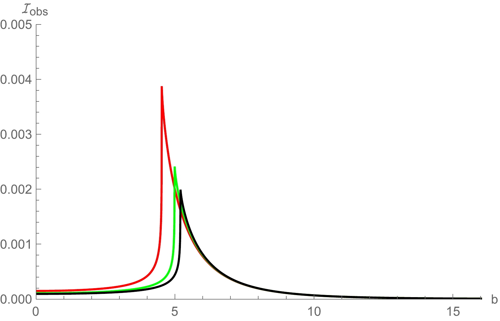
Figure 5. (color online) Observed specific intensity of the black hole surrounded by the infalling spherical accretion, in which the black, green and red lines correspond to
$ g/M=0 $ ,$ g/M=0.475 $ and$ g/M=0.75 $ , respectively. Here, we take$ M=1 $ .We find that the maximum value of observed intensity is still at the position of photon sphere (
$ b\sim b_p $ ). In addition, the observed intensity increases with the increase of impact parameter b in the region of$ b < b_p $ , and decreases with the increase of impact parameter b in the region$ b > b_p $ . However, the peak value of the observed intensity is much smaller than that of the static model, and the difference in peak value is more obvious under the different values of specific magnetic charge$ g/M $ . In other words, the black hole shadow with infalling spherical accretion is darker than that in the static case. A two-dimensional image of the observed intensity is also shown in Fig. 6.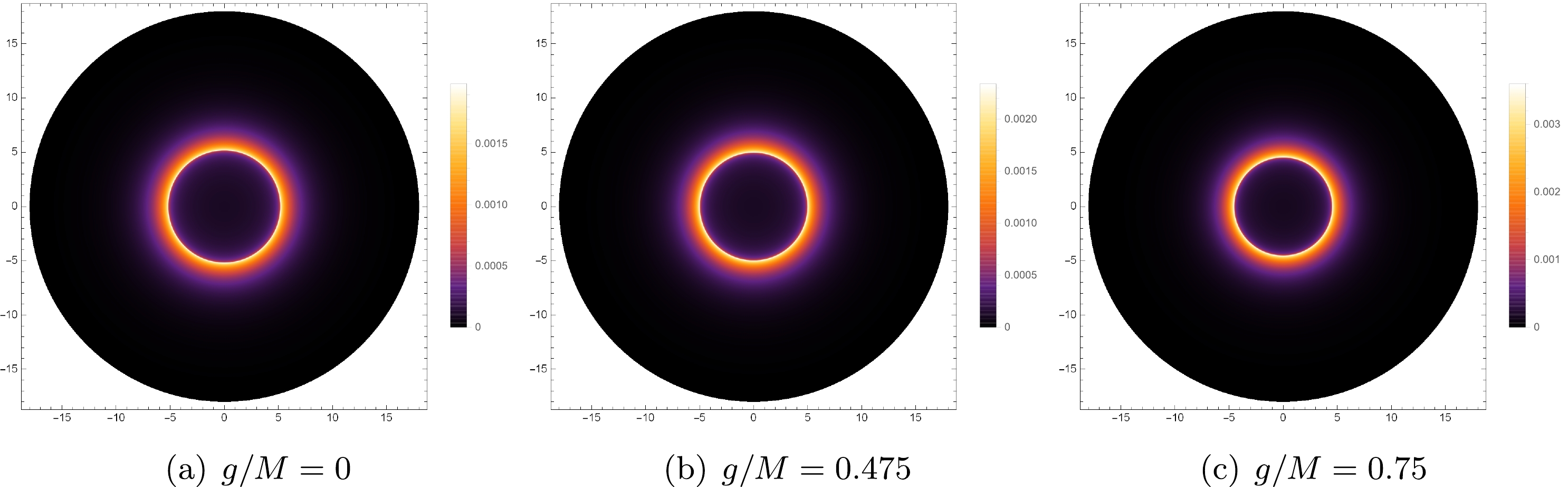
Figure 6. (color online) Image of the black hole shadow with infalling spherical accretion, for different values of specific magnetic charge
$ g/M $ , in which$ g/M=0 $ (left panel),$ g/M=0.475 $ (mid panel) and$ g/M=0.75 $ (right panel). Here, we take$ M=1 $ .We find that the central region inside the photon sphere in Fig. 6 is evidently darker than the corresponding region in Fig. 4, and the intensity of the bright ring is far less than that with static accretion. The obvious difference between these two models is due to the Doppler effect, as near the event horizon of the black hole, this effect is more obvious. In addition, we find that the radius of the shadow and the position of photon sphere remain unchanged in the different accretion processes. This suggests that the shadow is an inherent property of the spacetime, and the behavior of accretion flow around the black hole only affects the observed intensity.
-
In this section, we study the shadow when a black hole is surrounded by thin disk accretion in the Bardeen black hole, where an optically and geometrically thin disk is placed on the equatorial plane of black hole. The trajectories of light rays near the black hole are the important basis for studying the shadow and observed features of black hole. In Ref. [54], Gralla et al. distinguish the trajectories of light rays near the black hole, and they propose the total number of orbits which is defined as
$ n (b)=\frac{\varphi }{2 \pi }, $

(25) which is a function of impact parameter b. Using equation (25), the trajectories of the light ray are divided into three types, namely, direct, lensing and photon ring trajectories. That is, there are not only the photon rings but also lensing rings outside of the black hole shadow. In the case of
$ n(b) < 3/4 $ , the light ray will intersect the equatorial plane only once, corresponding to the direct emissions. In the case of$ 3/4 < n(b) < 5/4 $ , the light ray will cross the equatorial plane at least twice, corresponding to the lensing rings. In the case of$ n(b) > 5/4 $ , the light ray will intersect the equatorial plane at least three times, corresponding to the photon rings. For the different values of specific magnetic charge$ g/M $ , the range of impact parameters corresponding to direct, lensing rings and photon rings in the Baedeen spacetime is shown in Table 3. Also, we show the relationship between the total number of orbits$ n(b) $ and impact parameter b in the Bardeen spacetime in Fig. 7.$g/M$ 

Direct Lensing rings Photon rings 0 $b<5.0267$ or

$b>6.1927$ 

$5.0267<b<5.1893$ and

$5.2305<b<6.1927$ 

$5.1893 < b < 5.2305$ 

0.1 $b<5.0049$ or

$b >6.1623$ 

$ 5.0049<b<5.179$ and

$5.2196<b<6.1623$ 

$5.179< b < 5.2196$ 

0.475 $b<4.7564$ or

$b>6.0446$ 

$4.7564<b<4.9717$ and

$5.0276<b<6.0446$ 

$4.9717< b < 5.0276$ 

0.75 $b<4.0769$ or

$b>5.8461$ 

$4.0769<b<4.5142$ and

$4.6561<b<5.8461$ 

$4.5142< b <4.6561$ 

Table 3. Regions of direct, lensing rings and photon rings corresponding to impact parameters b under different values of specific magnetic charge
$g/M$ , where$M=1$ .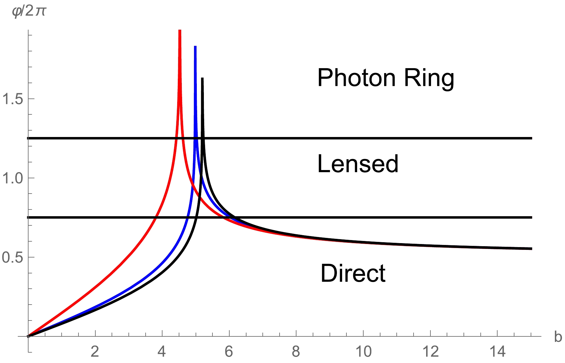
Figure 7. (color online) Behavior of photons in the Bardeen black hole as a function of impact parameter b in case of
$ M = 1 $ . The colors correspond to$ g/M = 0 $ (black),$ g/M=0.475 $ (blue), and$ g/M=0.75 $ (red), respectively.In Fig. 7, we find that the same value of b may correspond to different regions under different values of specific magnetic charge
$ g/M $ , as seen in Table 3. In addition, the values of impact parameter b corresponding to the photon rings and lensing rings are smaller than those in the Schwarzschild spacetime ($ g\rightarrow0 $ ), but the specific magnetic charge$ g/M $ leads to the increase of the ratio of the region occupied by the photon rings and lensing rings. When the impact parameter b increases to a large enough value, the light ray trajectories are the direct case no matter what the value of$ g/M $ is. That means, both the specific magnetic charge$ g/M $ and impact parameter b will affect the observed characteristics of the Bardeen black hole. In order to more clearly distinguish the distribution of light ray trajectories near the black hole, we show the associated photon trajectories for the Bardeen black hole in polar coordinates ($ b,\varphi $ ) in Fig. 8.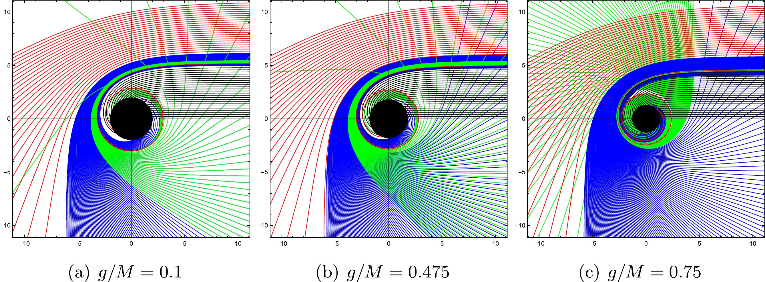
Figure 8. (color online) Selection of associated photon trajectories in polar coordinates
$ (b, \varphi) $ , in which the red, blue and green lines correspond to direct, lensing, and photon ring bands, respectively. The spacing in the impact parameter is 1/10, 1/100, and 1/1000 in the direct, lensing and photon rings, respectively. The black hole is shown as the black disk, and the dashed red line represents the photon ring. The black hole mass is taken as$ M = 1 $ . -
We consider that a distant static observer is located at the north pole, and the thin disk accretion at the equatorial plane of the black hole. Moreover, the light emitted from the thin disk accretion is isotropic for the static observer. In view of this, the specific intensity and frequency of the emission are expressed as
$I_{\nu }^{{\rm em}} (r)$ and$\nu_{\rm em}$ , so as the observed specific intensity and frequency are defined as$I_{\nu'}^{{\rm obs}} (r)$ and$\nu_{\rm obs}$ . By considering that${I_{\nu }^{{\rm em}}}/{\nu _e^3}$ is conserved along a ray from the Liouville theorem, we obtain a correlation between the observed specific intensity and the emissivity specific intensity [55],$ I_{\nu ' }^{{\rm obs}}= (A (r))^{3/2} I_{\nu }^{{\rm em}}(r). $

(26) Thus, we can obtain the total observed and emitted intensity by integrating for the full frequency,
$ I_{{O}}=\int I_{\nu ' }^{{\rm obs}} (r) \, {\rm d}\nu_{\rm obs} ' =\int (A (r))^2 I_{\nu }^{{\rm em}} \, {\rm d}\nu_{\rm em} =(A (r))^2 I_{\nu }^{{\rm em}} (r), $

(27) and
$ I_{{E}}=\int I_{\nu }^{{\rm em}} (r) {\rm d} \nu_{\rm em}. $

(28) It is worth mentioning that this only includes the intensity of light emitted from the accretion disk, and the absorption or reflection of light and other factors are not considered. When the trajectory of a light ray passes through the accretion disk on the equatorial plane, a certain luminosity will be obtained, and transmitted to the observer at infinity. As discussed earlier, the different values for the number of orbits
$ n(b) $ define the number of times that the ray path pass through the equatorial plane of the black hole. In the case of$ 3/4<n(b)<5/4 $ , the light ray will bend around the black hole and intersect with the back of the thin disk after the first intersection with the thin disk. In this way, the light ray will pass through the thin disk twice. When$ n(b)>5/4 $ , the light passes through the back of the thin disk and then through the front of the thin disk again, as the light ray is more curved around the black hole, i.e., the light will pass through the thin disk at least three times. Hence, the sum of the intensity at each intersection is the total intensity that the observer can observe, which is$ I_{{O}}(r)=\sum\limits_n (A (r))^2 I_{{E}}\Big|_{r= r_n(b)}. $

(29) Here,
$ r_n(b) $ is the transfer function, which represents the radial position of the$ n^\text{th} $ intersection with the thin emission disk, which means that the relationship between radial coordinate r and impact parameter b can be expressed by the transfer function. In addition,${\rm d}r/{\rm d} b$ corresponds to the slope of the transfer function, which is called the demagnification factor. Actually, the slope of the transfer function reflects the demagnified scale of the transfer function [54, 55]. In Fig. 9, graphs of the transfer functions are given under the different values of specific magnetic charge$ g/M $ .
Figure 9. (color online) Relationship between the first three transfer functions
$ r_n(b) $ and b in the Bardeen spacetime, in which the black, orange, and red lines correspond to the direct, lensing rings and photon rings, respectively. The black hole mass is taken as$ M = 1 $ .The black line corresponds to the first transfer function (
$ n=1 $ ), and its slope$\left(\dfrac{{\rm d} r}{{\rm d}b}\Big|_1 \right)$ is a small fixed value. This first transfer function corresponds to the direct image of the thin emission disk, which is the redshift of the source profile. The orange line corresponds to the second transfer function ($ n=2 $ ), for which the slope$\left( \dfrac{{\rm d} r}{{\rm d} b}\Big|_2 \right)$ is a very large value. Therefore, the observer will obtain a highly demagnified image on the back of the thin disk, which corresponds to the lensing rings. The red line represents the third transfer function ($ n=3 $ ), whose slope$\left( \dfrac{{\rm d} r}{{\rm d} b}\Big|_3 \right)$ is close to infinity$\left(\dfrac{{\rm d} r}{{\rm d} d}\Big|_3 \sim \infty \right)$ . The observer will see an extremely demagnified image of the front side of the disk. The third transfer function corresponds to the photon ring. As a result, the observed luminosity provided by the photon rings and lensing rings only accounts for a small proportion of the total observed flux, the direct emission is the main measure of observed intensity. In addition, the image provided by the later transfer functions are more demagnetized and negligible, so we only consider the first three transfer functions. -
With the help of this preparatory work, we can further study the specific intensity of emission. For the form of emission, we mainly consider three different models. In Model I, the peak of emission intensity is at the position of the innermost stable circular orbit (
$r_{\rm isco}$ ). There will be no emission inside the innermost stable circular orbit, but there exists a sharp downward trend outside the innermost stable circular track:$ {I_E}({r_1}) = \left\{ {\begin{array}{*{20}{l}} {{{\left( {\dfrac{1}{{r - ({r_{\rm isco}} - 1)}}} \right)}^2},}&{r > {r_{\rm isco}}}\\ {0,}&{r < {r_{\rm isco}}} \end{array}} \right. $

(30) In Model II, we assume that the position of the emission peak is located at the photon sphere (
$ r_p $ ), and the emission is a decay function of the third power:$ {I_E}({r_2}) = \left\{ {\begin{array}{*{20}{l}} {{{\left( {\dfrac{1}{{r - ({r_p} - 1)}}} \right)}^3},}&{r > {r_p}}\\ {0,}&{r < {r_p}} \end{array}} \right. $

(31) In Model III, there is a gradual decay of the emission between the event horizon
$ r_h $ and the innermost stable circular orbit$r_{\rm isco}$ , such as$ {I_E}({r_3}) = \left\{ {\begin{array}{*{20}{l}} {\dfrac{{\dfrac{\pi }{2} - {{\tan }^{ - 1}}(r - ({r_{\rm isco}} - 1))}}{{\dfrac{\pi }{2} - {{\tan }^{ - 1}}({r_{ph}})}},}&{r > {r_h}}\\ {0,}&{r < {r_h}} \end{array}} \right. $

(32) Taking the specific magnetic charge
$ g/M = 0.475 $ as an example, the results for the intensity of the emission and observation are shown in Fig. 10. The left column is the trend of emission profiles$ I_E(r) $ with the increase of radius r, The middle column is the relationship between the observed intensity$ I_O(r) $ and the impact parameter b. The right column is the two-dimensional density plot of observed intensities$ I_O(r) $ in celestial coordinates. The first, second and third row correspond to the emission Models I, II and III, respectively. As can be clearly seen from Fig. 10, there is a disparity for both the central black area and observed intensity in the different emission models.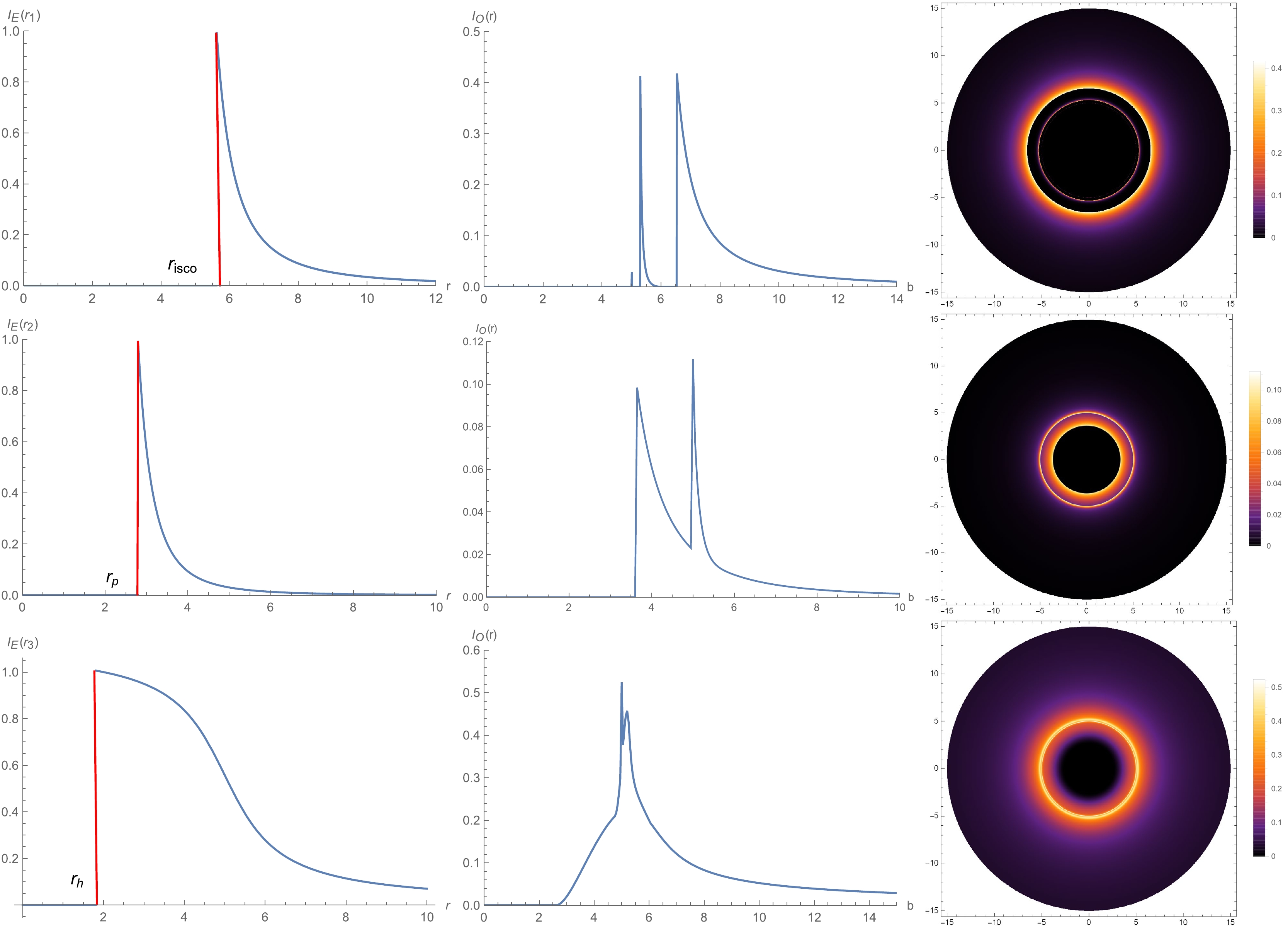
Figure 10. (color online) Observed appearance of the thin disk with different emission profiles near the black hole, viewed from a face-on orientation. The value of specific magnetic charge
$ g/M=0.475 $ , and$ M=1 $ .In Model I where the emission starts at the position of the innermost stable circular orbit, although the photon rings can gain more brightness from the thin disk, they are highly demagnetized. As can be see from the middle column, the observed intensity in the photon ring region is very small and confined to a narrow region. Moreover, the two-dimensional density map also shows that there is an almost invisible thin line in the photon ring region. Therefore, the contribution of the photon ring to the total observed flux is negligible. For the lensing rings, the observed intensity is larger than that of the photon rings, but the area occupied by the lensing rings is also very narrow, which leads to a bright line in the area of the lensing rings in the two-dimensional density map. As the result, the observed intensity obtained by the observer at infinity is mainly provided by direct emission.
In Model II where the emission starts at the photon sphere, the emission regions of the lensing rings and the photon rings overlap, which resulting in a bright band outside the shadow as shown in the two-dimensional density map. The contribution of the lensing rings to the total observed flux is higher than that of Model I, while the contribution of the photon ring is still negligible. That is to say, the observed intensity obtained by the distant observer will still be determined by direct emission.
In Model III where the emission starts from the event horizon of black hole, the observed intensity increases with the increase of b from the outer edge of event horizon until it reaches to the peak near the lensing ring. The photon rings and lensing ring completely coincide and cannot be distinguished. In addition, the contribution of the lensing rings to the total observed flux is partially helpful while the photon ring makes a negligible contribution, but direct emission continues to dominate the total observed intensity.
The profiles of emission and observed intensities when the specific magnetic charge
$ g/M=0.75 $ are shown in Fig. 11. By comparing Fig. 10 with Fig. 11, it can be found that the observed intensity, range of the central dark area and size of the light band outside the shadow are all clearly different. As the value of specific magnetic charge$ g/M $ increases, the range of the central dark area and size of the light band outside the shadow decrease. Moreover, the observed intensity obtained by the distant observer also decreases. As the proportion of area for the photon rings and lensing rings increases with larger values of specific magnetic charge$ g/M $ , the proportion of area from direct emission decreases relatively, which naturally leads to the weakening of observed intensity determined by direct emission.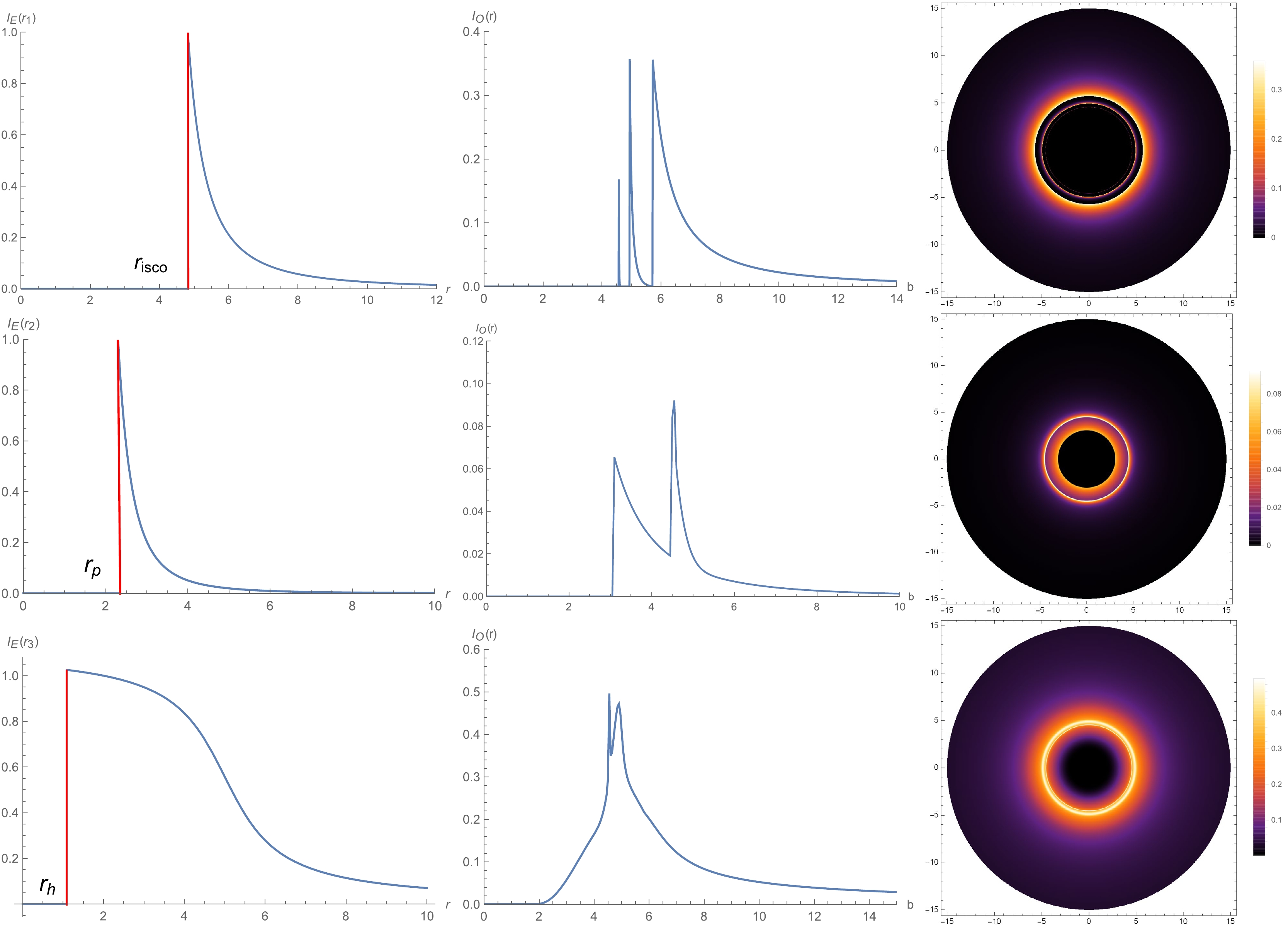
Figure 11. (color online) Observed appearance of the thin disk with different emission profiles near the black hole, viewed from a face-on orientation. The value of specific magnetic charge
$ g/M=0.75 $ , and$ M=1 $ .To distinguish the Bardeen black hole from the Schwarzschild black hole, here we have employed
$ M = $ 0.87991 and plotted the shadows and light rings of the Schwarzschild black hole under the three models, as shown in Fig. 12. When$ M=0.87991 $ for the Schwarzschild black hole, the shadow radius$ b_p $ is equal to that of the Bardeen black hole (i.e.,$ g/M=0.75 $ ). In this case, if there is no matter, or only spherical accretions around the black hole, the size of shadow is exactly the same for the Bardeen and Schwarzschild black holes. However, by comparing Figs. 11 and 12, we find that with a thin disk the observed intensities (i.e., the middle columns for Figs. 11 and 12) for all three emission models are very different. For instance, the light rings observed in the Schwarzschild case are larger, due to the radius of the photon sphere and the event horizon of the Schwarzschild black hole being larger than those of the Bardeen spacetime. More importantly, the results show that for Model III the direct emission and rings all overlap for the Schwarzschild black hole, but are distinguishable in the Bardeen case. In addition, the intensities of direct emission and the rings are very different for these two black holes. From these facts, we can conclude that the shadows and rings could be an effective characteristic for distinguishing the Bardeen black hole from the Schwarzschild black hole, and that the magnetic charge g has a close correlation with the observed intensity.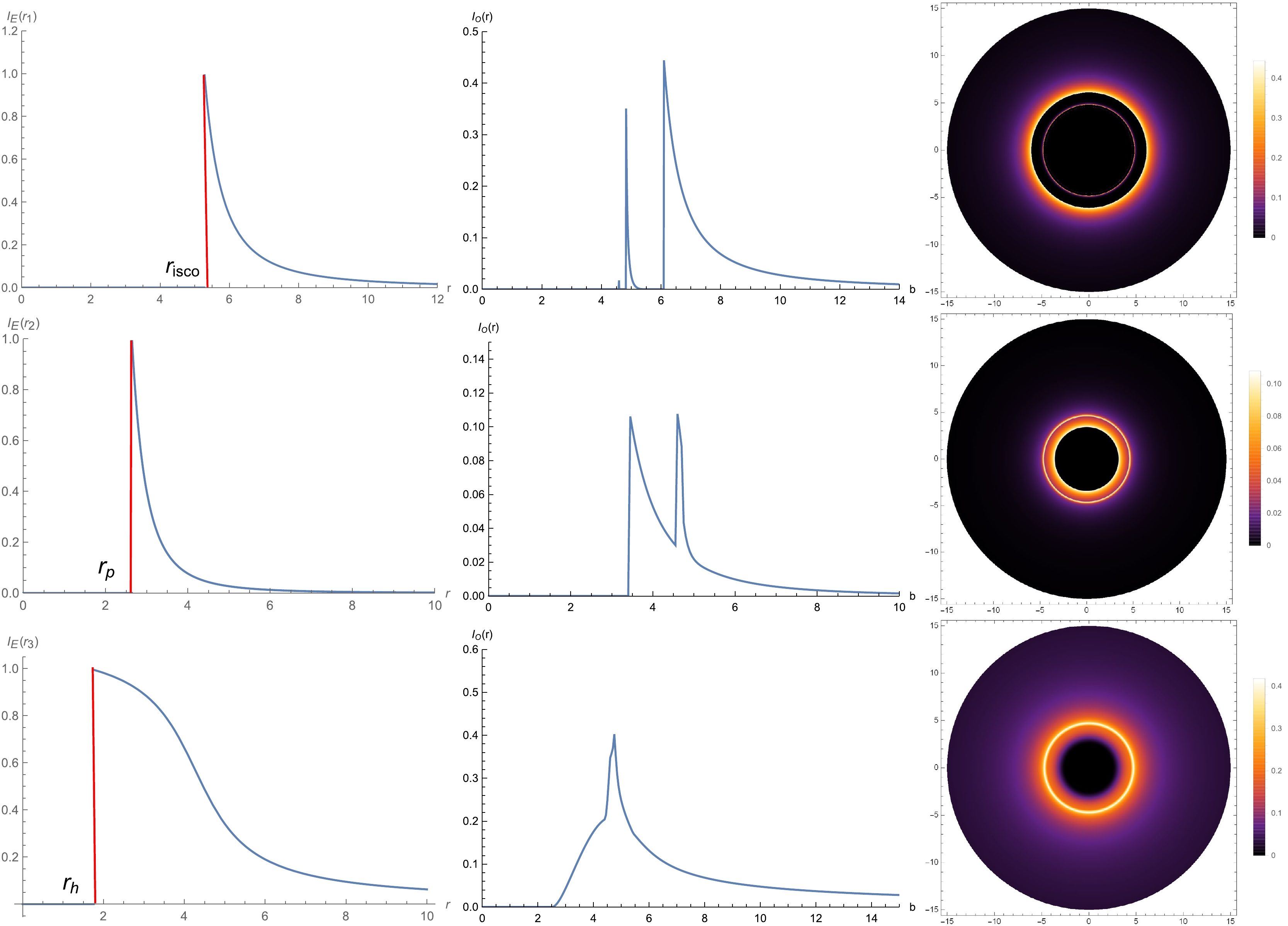
Figure 12. (color online) Observed appearance of the thin disk with different emission profiles near a black hole in the Schwarzschild spacetime with
$ M=0.95938 $ , viewed from a face-on orientation. -
It is commonly known that black holes are surrounded by accretion matter, and the distribution of accretion plays a key role in the imaging of black holes. In the context of the Bardeen spacetime, we have investigated the black hole shadow and observed luminosity under different accretion models. In particular, we pay close attention to the different observed characteristics for a distant observer when the related physical quantities have different values.
When the black hole is surrounded by spherically symmetric accretion flow, we consider two behaviors of the accretion, i.e., the static and infalling accretion models. For the case of static spherically symmetric accretion, we find that the observed luminosity increases with the increase of the specific magnetic charge
$ g/M $ , while the photon sphere and radius of the black hole decrease. In addition, the maximum observed luminosity always appears in the region of the photon sphere under the different values of specific magnetic charge$ g/M $ . From the observed intensity density map, one can see that the central region of the shadow is not completely dark, and the observed brightness of the central region increases slightly with the increase of$ g/M $ . In the infalling accretion model, the maximum observed luminosity is clearly lower than that of the static model, which is the most prominent difference between these two models. The Doppler effect for the infalling matter leads to this difference between the two kinds of spherical accretion. As a result, the observed image in the infalling accretion model is darker than the static one under the same state parameters. This change of observed intensity is more obvious when the specific magnetic charge$ g/M $ takes a larger value. The maximum observed luminosity with$ g/M = 0.75 $ is about twice that of$ g/M = 0 $ (Schwarzschild black hole). It must also be mentioned that in both spherical accretion models, there is a great difference in the observed luminosity, but the position of photon sphere and the shadow radius are unchanged under the same parameters, which means that the shadow is an inherent property of the spacetime and not affected by the accretion flow behavior.By considering the Bardeen black hole surrounded by a geometrically and optically thin disk accretion, we have distinguished the trajectory of light rays near black hole. Then, we take three different emission models for the thin disk accretion flow. For an observer at infinity (
$ r_0\rightarrow \infty $ ), there is not only a dark central area, but also the photon rings and lensing rings outside of black hole shadow. In the different emission models, the maximum observed luminosity and the size of central dark area are different. The thin disk serves as the only background light source. Light rays in the region of the photon rings can accretes through the thin disk more than three times, gaining extra brightness. However, the photon rings cannot be observed directly by the observer, as the photon ring region is very narrow and its image is extremely demagnetized. In addition, the image of the lensing ring region also experiences high demagnetization, such that the lensing rings can only provide a very small part of the total observed flux. Therefore, the observed intensity is dominated by direct emission in all three different emission models. Although these results are obtained with ideal models, it is very important to push forward the theoretical study of the black hole shadow as far as possible and lay the foundation for observed results.
Shadow images and observed luminosity of the Bardeen black hole surrounded by different accretions
- Received Date: 2022-02-20
- Available Online: 2022-08-15
Abstract: In this paper, by exploring photon motion in the region near a Bardeen black hole, we studied the shadow and observed properties of the black hole surrounded by various accretion models. We analyzed the changes in shadow imaging and observed luminosity when the relevant physical parameters are changed. For the different spherical accretion backgrounds, we find that the radius of shadow and the position of the photon sphere do not change, but the observed intensity of shadow in the infalling accretion model is significantly lower than that in the static case. We also studied the contribution of the photon rings, lensing rings and direct emission to the total observed flux when the black hole is surrounded by an optically thin disk accretion. Under the different forms of the emission modes, the results show that the observed brightness is mainly determined by direct emission, while the lensing rings will provide a small part of the observed flux, and the flux provided by the photon ring is negligible. By comparing our results with the Schwarzschild spacetime, we find that the existence or change of relevant status parameters will greatly affect the shape and observed intensity of the black hole shadow. These results support the theory that the change of state parameter will affect the spacetime structure, thus affecting the observed features of black hole shadows.


 DownLoad: