-
As a unique means of generating quark-gluon plasma (QGP) on earth, high-energy heavy-ion collision experiments provide opportunities to study this type of extremely hot and dense matter. With further research on the collective behaviour of quarks and gluons, the deep structure of a nucleus and the state of the universe a few microseconds after the Big Bang have been discovered. For heavy-ion collisions, besides collision energy, the impact parameter (denoted by b) is a crucial quantity that determines the initial geometry of a collision. Numerous quantities have essential correlations with the impact parameter. For example, the elliptic flow of hadrons is sensitive to the impact parameter [1]. Electromagnetic (EM) fields in heavy-ion collisions roughly satisfy
$ e\vert {\rm Field} \vert \propto \sqrt{s} f(b/R_A) $ , where$ f(b/R_A) $ is a function of$ b/R_A $ with$ R_A $ as the nucleus radius [2, 3]. When studying the EM properties of QGP, dilepton production is a significant probe. For lepton pair production, both the cross section and azimuthal asymmetry have a strong dependence on the impact parameter [4]. The recently observed hyperon spin polarization increases with increasing impact parameter of collisions [5, 6]. However, the impact parameter of a single collision cannot be measured directly in heavy-ion experiments. Usually, it is estimated using particular final-state observables sensitive to it, such as charged-particle multiplicity. By introducing the concept of centrality, which is defined as classes categorized by b, and comparing experimental data with simulation results using, for example, the Glauber model, one can determine the rough interval of the impact parameter of an event [7].Owing to their powerful ability to establish a reliable map between input data and the target value without significant prior knowledge, deep learning (DL) methods are widely used in both science research and our daily life. When applying DL algorithms to face recognition tasks, a machine can identify a person's ID with his/her facial information [8]. For heavy ion collisions, the impact parameter can be viewed as one of the IDs of an event. Several studies have proved the effectiveness of DL methods on impact parameter 'recognition' [9–17]. From a simple neural network [9] to a PointNet model [13] and boosted decision trees [17], with the development of machine learning algorithms, more appropriate learning methods have been proposed to improve the performance of 'recognition' and satisfy experimental requests. However, most of this research only involves collisions at low or intermediate energies [9–16]. Although a recent study [17] considered LHC energies, the adopted machine learning model is not a deep neural network (DNN).
Here, we investigate RHIC Au+Au collisions at
$ \sqrt{s_{NN}} = 200 $ GeV and choose final-state charged hadrons as probes. After transforming the momentum information of these particles into energy spectra as input data for the learning models, we use a multi-layer perceptron (MLP) model and convolutional neural network (CNN) model to obtain a map between the energy spectrum and impact parameter, respectively. Then, we analyze the influences of beam energy and the range of pseudorapidity on the accuracy of predictions. Furthermore, we examine the interpretability of the CNN serving as a regression machine. An 'attention' map of the CNN model is obtained using the Grad-Cam algorithm, and all of the collisions are simulated by a multi-phase transport (AMPT) model [18]. -
The discovery of the Higgs Boson in 2012 completed the jigsaw of elementary particles according to the current Standard Model. Soon after, CERN announced the Higgs boson machine learning challenge [19] to the public. The goal of this challenge is to help experimentalists better distinguish the signal of Higgs boson decay from background noise using machine learning (ML) methods. ML was found to be extremely effective in this task.
As a branch of the field of artificial intelligence, ML technology has promoted intelligentization in many areas of industry, such as autonomous driving, smart mobile electronic devices, and the internet. Because scientists often deal with large quantities of data or require information that is difficult to obtain using traditional methods, they have applied ML techniques to fundamental science research, and physics is no exception. On the whole, the applications of ML in physics can be divided into two categories. The first is the replacement of physical models with ML models if the latter are more effective for specific problems. By training ML models with a large quantity of data, a map can be constructed between two or more physical quantities. For instance, by training neural networks to approximately imitate wave functions, we can construct a map between the potential and one particle's energy without solving the Schrödinger equation [20] or quantum many-body problem [21]. The second is to recognize the target signal (such as a physical phenomenon) from the background with noise. For example, deep neural networks can help distinguish the Higgs boson or other exotic particles of interest (signal) from other particles (background) [22]. In short, ML algorithms can be used to deal with regression and classification problems in physics. As a branch of ML, DL has become the most popular AI method in physics research. In the field of relativistic heavy ion collisions, DL has been applied to the problems of QCD phase transition [23–25], relativistic hydrodynamics [26], jet structure [27, 28], the search for the chiral magnetic effect [29], and recognition of the initial clustering structure in nuclei [30]. Among various DL algorithms, the DNN, especially the convolutional neural network, are commonly used.
The DNN is one of the early DL models. Owing to its remarkable ability to realize nonlinear mapping with a comparatively simple structure, the DNN is still a preferred tentative model for most regression tasks. A DNN (Fig. 1), also known as a multi-layer perceptron (MLP), is composed of an input layer, sufficient hidden layers to be considered 'deep', and an output layer.
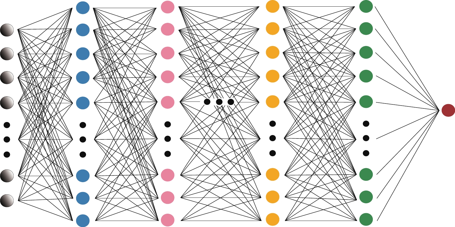
Figure 1. (color online) Architecture of the multi-layer perceptron (MLP) we use in this study. It contains four hidden layers. The first layer is composed of 512 neurons, the second layer has 256 neurons, the third layer has 128 neurons, and the final hidden layer has 64 neurons.
The CNN commonly appears in 2D image-related tasks. A typical CNN consists of the input layer, convolutional layers, pooling layers, fully connected layers, and the output layer. Our CNN architecture is shown in Fig. 2.

Figure 2. (color online) Structure of the convolutional neural network (CNN). It contains two convolutional layers and four fully-connected layers.
As a supervised learning regression task, impact parameter determination aims at constructing a map between the input observables and a single value, that is, the impact parameter of an event. Thus, it is appropriate to choose the mean squared error (MSE) as the loss function to examine the performance of the learning models. This is defined as
$ \begin{equation} {\rm Loss} = \frac{1}{N_{\rm batch}} \sum\limits_{i=1}^{N_{\rm batch}}(y_i^{\rm pred} - \hat{y}_i^{\rm true})^2 , \end{equation} $

(1) where
$ \hat{y}_i^{\rm true} $ is the true value of the impact parameter of an event among a batch of events with a size of$ N_{\rm batch} $ , and$ y_i^{\rm pred} $ is the output of the MLP/CNN model, corresponding to the prediction value. -
We consider Au+Au collisions at
$ \sqrt{s_{NN}}=200 $ GeV and use a multi-phase transport (AMPT) model to perform the simulation. The AMPT model [18] is a hybrid transport model that contains four basic stages: the initial condition, partonic scattering, hadronization, and hadronic interaction. The initial condition is generated using the HIJING model [31]. Scatterings among partons are modeled by Zhang's Parton Cascade (ZPC) model [32]. Two different versions of the AMPT model are available for the process of hadronization. The first is the default model, in which partons are recombined with their parent strings and the Lund string fragmentation model is used to turn partons into hadrons. The second contains a string melting model. This combines partons with hadrons via a quark coalescence model. Finally, the rescatterings of hadronic matter are performed by a relativistic transport (ART) [33]. Here, we choose the model with string melting as the simulator.The selection of features serving as input information is the first step in a deep learning process. Considering the experimental observability, we choose the momenta of the freezed-out charged hadrons with pseudorapidity η satisfying
$ -1 \leq \eta \leq 1 $ as observables.As shown in Sec. II, the input data of an MLP model and that of a CNN model have different forms. Here, for the CNN model, the observables above are transformed into two-dimensional (2D) energy spectra in (
$ p_x $ ,$ p_y $ ) space. Fig. 3 illustrates the case of an event with$ b=1.65 $ fm. The$ x, y $ components of momenta are cut by the interval$ [-1.5, 1.5] $ , and the ($ p_x $ ,$ p_y $ ) space is cut by a$ 25 \times 25 $ grid. Each cell in this grid contains the sum of the energies of charged particles whose$ p_x $ and$ p_y $ are within corresponding intervals. Note that the energy contains not only the momentum but also the mass of the particle. Thus, an energy spectrum carries more physical information than a multiplicity spectrum. By arranging the pixels of a 2D energy spectrum into a 1D chain, data is generated as an input for the MLP model.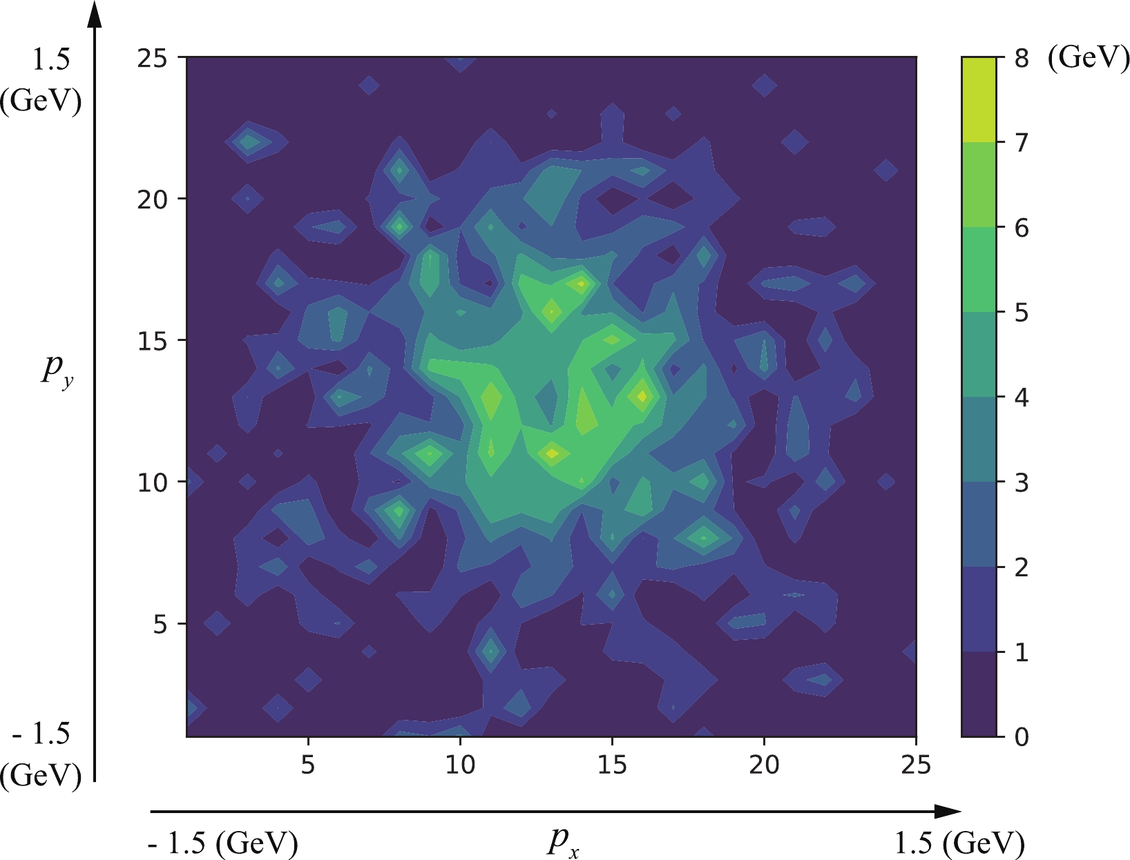
Figure 3. (color online) Energy spectrum in (
$ p_x $ ,$ p_y $ ) space of final-state charged particles of an event with$ b=1.65 $ fm. This is cut by a$ 25 \times 25 $ grid. Each unit in the grid represents the sum of the energies of the enclosed particles. This type of energy spectrum is used as the input data for DL models. -
We generate 28000 events per centrality and divide them into two parts: 20000 events for training and 8000 events for validation. The interval of the impact parameter
$ b \in [0, 12.5] $ fm is divided into nine centrality classes [34]. Thus, the total training dataset is composed of 180000 events, and the total validation dataset contains 72000 events. After appropriate training of the model, 20000 events (satisfying a differential distribution$ \propto b db $ in the impact parameter) are input into the model to test its prediction accuracy.In Fig. 4, we show the errors of the predicted impact parameters compared to the true values. Both the MLP and CNN models exhibit high prediction accuracy for semi-central and semi-peripheral events. The mean error of the CNN model for events with the impact parameter satisfying
$ 2 $ $ \leq b \leq 11 $ fm ranges from$ -0.06 $ to$ 0.05 $ fm, and that of the MLP model ranges from$ -0.08 $ to$ 0.08 $ fm. The mean absolute prediction error is$ 0.40 $ fm for the CNN model and$ 0.41 $ fm for the MLP model, indicating that the CNN model performs slightly better than the MLP model. However, the accuracy decreases in central regions. The prediction values are greater than the true values for central collisions and vice versa for peripheral events.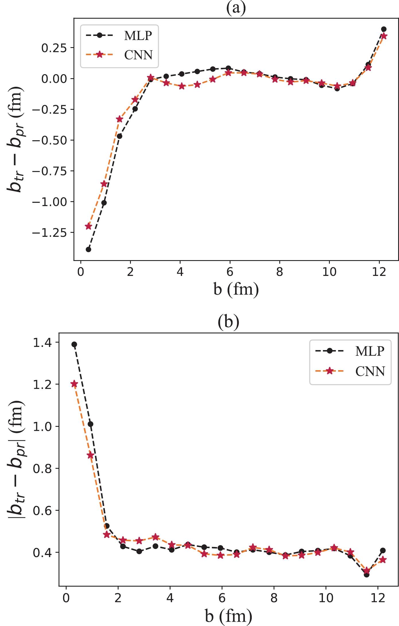
Figure 4. (color online) Errors between the true values of the impact parameter and those predicted by the MLP/CNN model for Au+Au collisions at
$ \sqrt{s_{NN}} = 200 $ GeV: (a) The mean errors between the true values (denoted by$ b_{\rm tr} $ ) and predicted values (denoted by$ b_{\rm pr} $ ); (b) Corresponding mean absolute errors. -
In heavy ion collisions, the beam energy is another crucial quantity that largely determines the bulk properties of the matter created in an event. Low-energy collisions differ from high-energy collisions in many aspects. With a higher beam energy, colliding nuclei generate more partons, and eventually more varieties of hadrons freeze out. To illustrate this, we generate a dataset for events with collision energies
$ \sqrt{s_{NN}} = 7.7,\ 39.0,\ 62.4, 130.0, \ 200.0 $ GeV, corresponding to the beam energy scan program performed at the RHIC. Then, we analyze their differences in the multiplicity and composition of final state charged particles. As shown in Fig. 5, the multiplicity of charged particles increases with beam energy. In addition, the fraction of protons in charged hadrons is higher at lower collision energies; however, the fraction of charged pions is not monotonic in collision energy. Hence, we test whether the differences in multiplicity and composition of the produced hadrons at lower collision energies affect the ability of the DL models.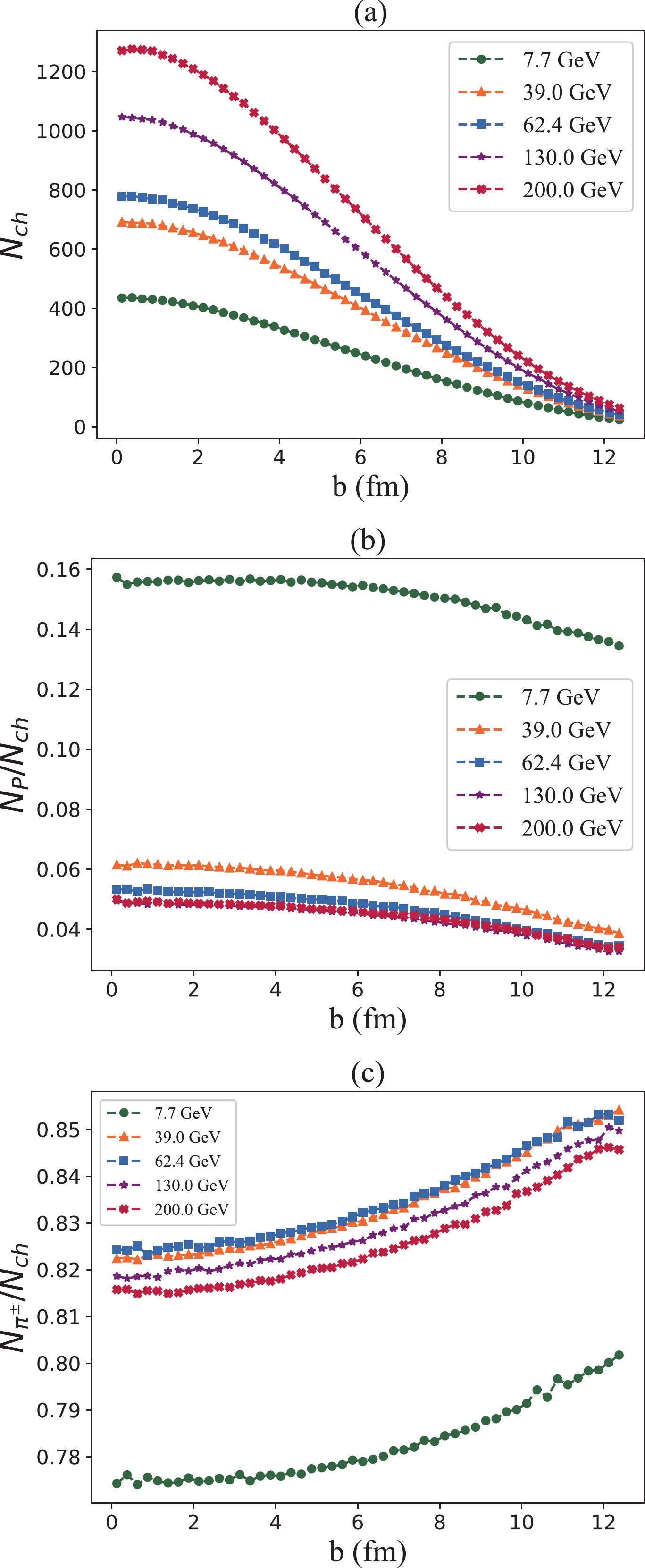
Figure 5. (color online) Multiplicity and composition of charged particles produced in collisions with different beam energies, that is,
$ \sqrt{s_{NN}} $ = 7.7, 39.0, 62.4, 130.0, 200.0 GeV: (a) The multiplicity of charged particles; (b) The fraction of protons in charged particles; (c) The fraction of charged pions.Therefore, we train and test the DL models to the cases of
$ \sqrt{s_{NN}} = 7.7,\ 39.0,\ 62.4,\ 130.0, \ 200.0 $ GeV. The results are shown in Fig. 6 and Fig. 7 for the MLP and CNN models, respectively. The DL models perform well for low and intermediate energy cases. Thus, we find that the DL models are robust against different collision energies.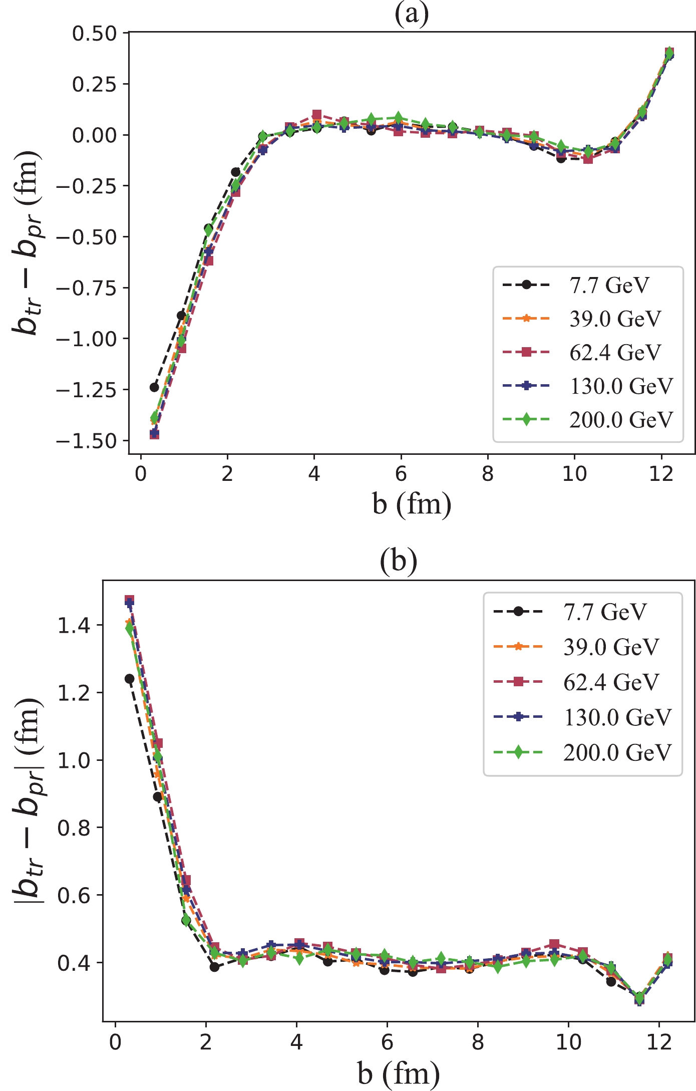
Figure 6. (color online) Performance of the MLP model in dealing with collisions with different beam energies, that is,
$ \sqrt{s_{NN}} $ = 7.7, 39.0, 62.4, 130.0, 200.0 GeV: (a) The mean errors between the true values (denoted by$ b_{\rm tr} $ ) and predicted values (denoted by$ b_{\rm pr} $ ); (b) Corresponding mean absolute errors.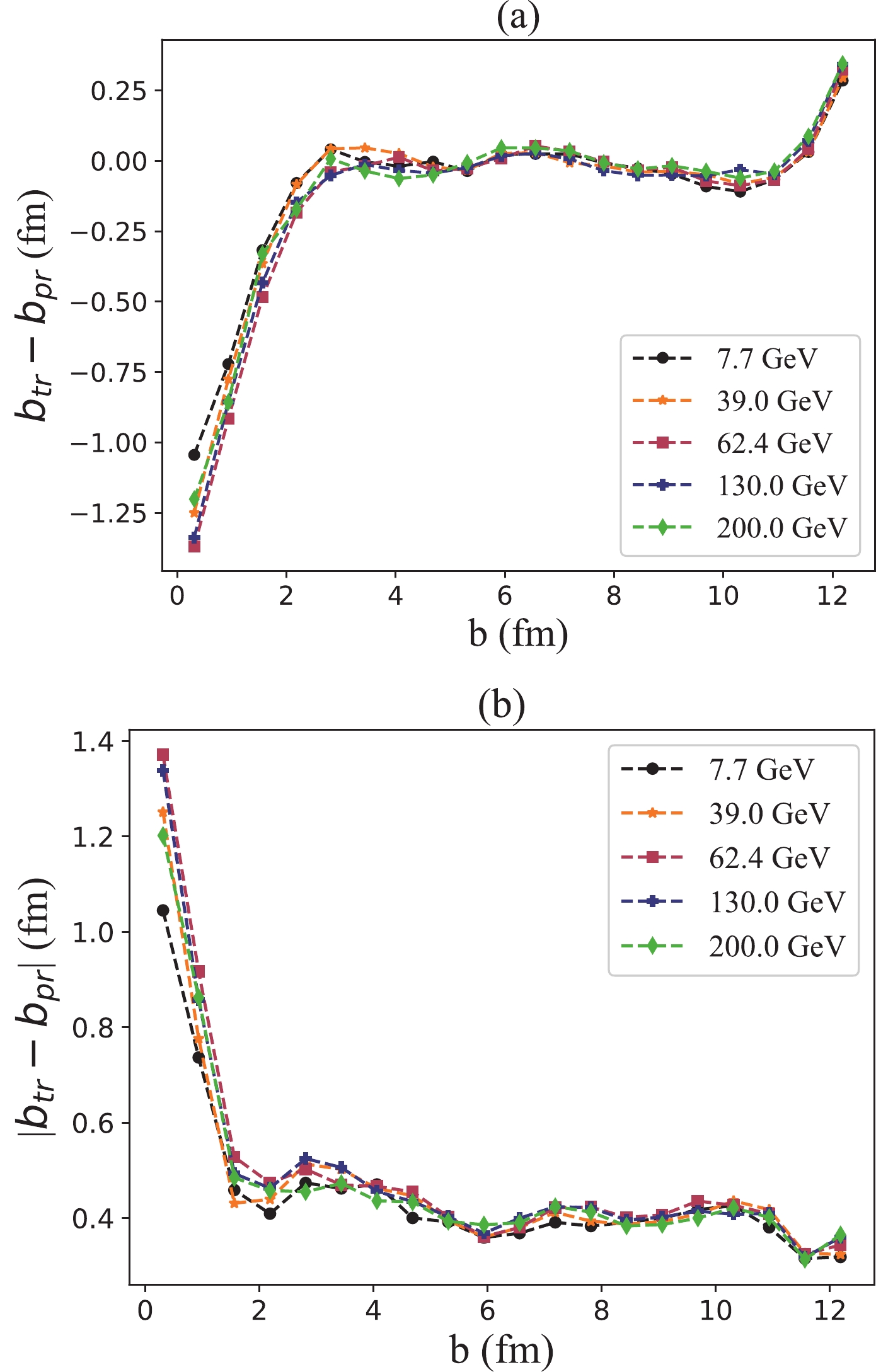
Figure 7. (color online) Performance of the CNN model in dealing with collisions with different beam energies, that is,
$ \sqrt{s_{NN}} $ = 7.7, 39.0, 62.4, 130.0, 200.0 GeV: (a) The mean errors between the true values (denoted by$ b_{\rm tr} $ ) and predicted values (denoted by$ b_{\rm pr} $ ); (b) Corresponding mean absolute errors. -
In most relativistic heavy ion collision experiments, attention is mainly focused on the mid-rapidity region, that is,
$ -1 \leq \eta \leq 1 $ , owing to the coverage limit of most detectors. However, the mid-rapidity region only covers a small part of final-state charged particles [35] (see Fig. 8). Therefore, more information can be obtained from the energy spectrum if we can observe a larger region in pseudorapidity. The octagon detector in the PHOBOS experiment can accept charged particles with$ |\eta| < 3.2 $ [36], and the recent upgrade of the inner Time Projection Chamber (iTPC) detector at the RHIC can extend the rapidity acceptance to$ -1.5 \leq \eta \leq 1.5 $ [37]. Thus, we take the regions of$ -3 \leq \eta \leq -1 $ and$ 1 \leq \eta \leq 3 $ into consideration.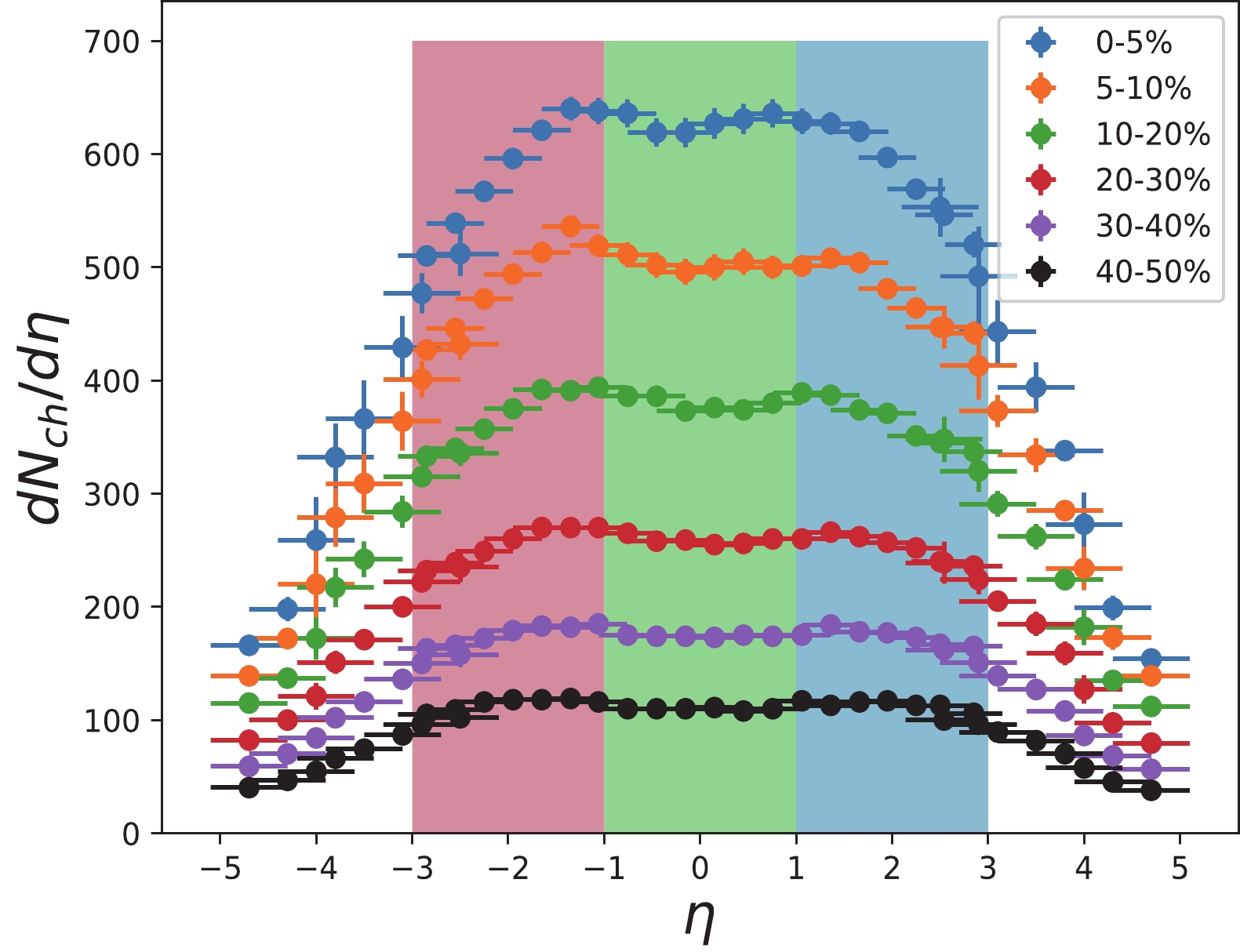
Figure 8. (color online) Distributions of
${\rm d}N_{\rm ch} / {\rm d}\eta$ for centrality ranges of, top to bottom, 0%–5%, 5%–10%, 10%–20%, 20%–30%, 30%–40%, and 40%–50% [35]. The particles in the pseudorapidity window of$ -3 \leq \eta \leq 3 $ are divided into three parts, [-3, -1], [-1, 1], and [1, 3], corresponding to three channels, 'R', 'G', and 'B', of the input layer.Now, we expand the training and detection region to
$ -3 \leq \eta \leq 3 $ . Because particles with positive pseudorapidity move in the opposite direction to those with negative pseudorapidity, we add two extra channels into the input layer of the CNN. Similar to inputting a colored picture with three channels 'RGB' into the CNN, we choose the region$ -3 \leq \eta \leq -1 $ as channel 'R,'$ -1 \leq \eta \leq 1 $ as channel 'G,' and$ 1 \leq \eta \leq 3 $ as channel 'B' (Fig. 8). Then, we feed the energy spectra with the three channels above to the CNN we trained with only data in the 'G' region. The CNN exhibits a higher prediction accuracy than that with one channel (Fig. 9). The mean absolute prediction error of the CNN for$ 2 \leq b \leq 12.5 $ fm is$ 0.35 $ fm. This value is 0.40$ \rm fm $ in the case of the CNN with only one input channel. Thus, extending the pseudorapidity window can truly improve the performance of regression.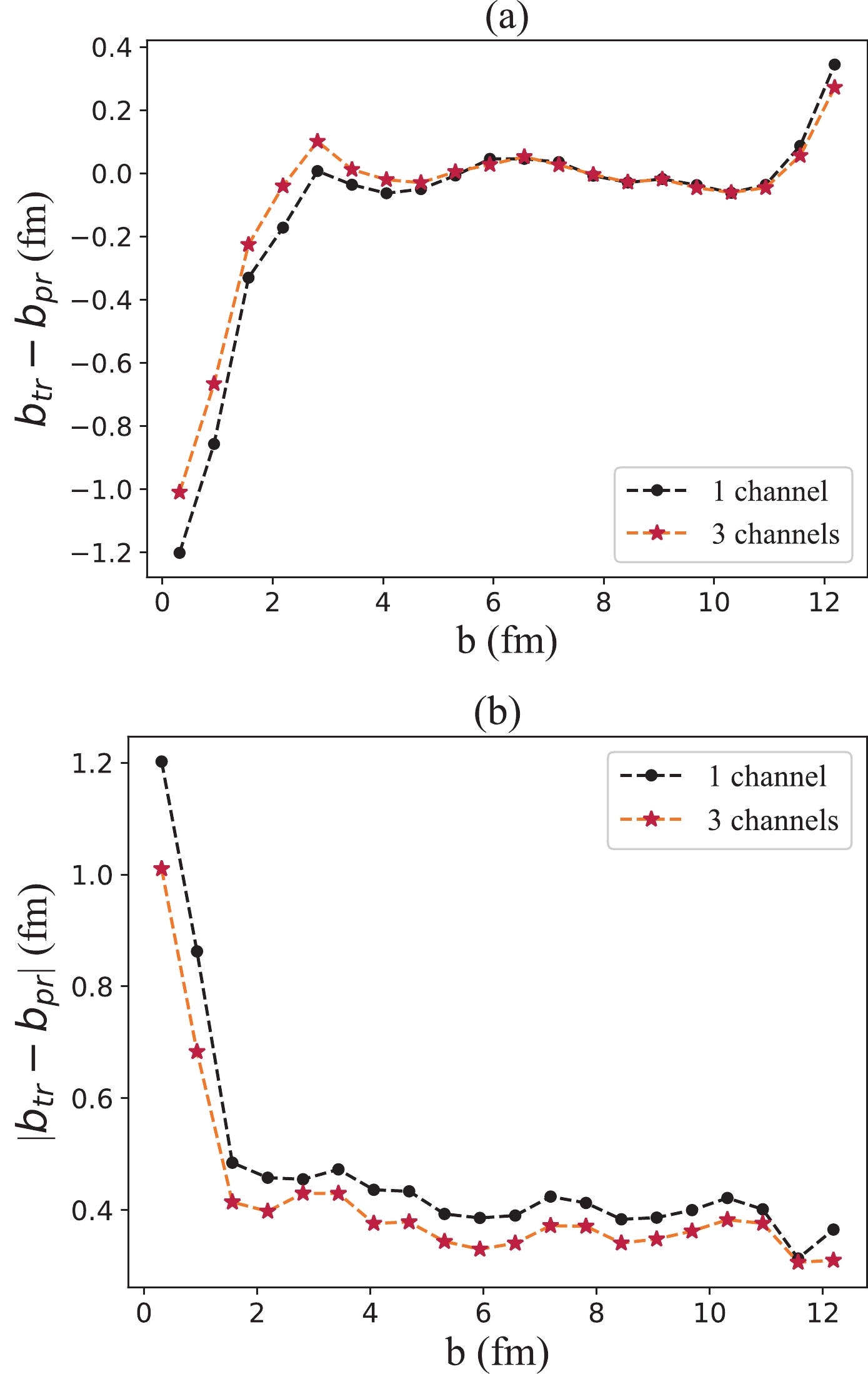
Figure 9. (color online) Errors between the true values of the impact parameter and those predicted by the CNN model with
$\sqrt{s_{NN}} = 200$ GeV. The number of input channels is one and three, respectively: (a) The mean errors between the true values (denoted by$ b_{\rm tr} $ ) and predicted values (denoted by$ b_{\rm pr} $ ); (b) Corresponding mean absolute errors. -
As mentioned previously, the impact parameter of a single event cannot be directly measured experimentally. This also applies to geometric quantities, such as the participant number
$ N_{\rm part} $ and binary collision number$ N_{\rm coll} $ . Instead, one can introduce the quantity of 'centrality,' which is usually expressed as a percentage of the total nuclear interaction cross section [7] and is strongly correlated with the impact parameter b, to estimate an event's b range. In heavy ion collision experiments, the multiplicity of final state charged particles ($ N_{\rm ch} $ ) is usually chosen as the main observable to classify event centrality. It is assumed that the average multiplicity of charged particles decreases monotonically when the impact parameter increases. With the Glauber model and Monte Carlo method, we can establish the centrality classes for heavy ion collisions [38]. By comparing the charged-particle multiplicity of an event measured by experiments with the results given by the MC-Glauber model, one can determine this event's centrality and further estimate its impact parameter.Here, we propose a scheme to compare the uncertainty on b determined using the multiplicity method with the CNN method. Based on the above assumption that the impact parameter is monotonically related to charged-particle multiplicity, if we select a batch of events with the same multiplicity (
$ N_{\rm ch} $ ), their impact parameters should satisfy a Gaussian-like distribution. We select the standard deviation ($ \sigma_{b}^{\rm mult} $ ) of these impact parameters as the quantity to characterize the uncertainty of mapping$ N_{\rm ch} $ to the corresponding impact parameter, which can be taken as the center of the Gaussian-like distribution, that is,$ \mu_{b}^{\rm mult} $ . Then, a batch of events with the same impact parameter$ \mu_{b}^{\rm mult} $ are generated by the AMPT model. With a well-trained CNN model, we can obtain the corresponding predicted impact parameters and calculate their standard deviation, that is,$ \sigma_{b}^{\rm CNN} $ . By comparing$ \sigma_{b}^{\rm mult} $ with$ \sigma_{b}^{\rm CNN} $ , we can evaluate the uncertainty on impact parameter determination using the multiplicity or CNN method.Owing to event-by-event fluctuation in the nucleon distribution of nuclei before collision and the complex evolution process after the collision, events with the same impact parameter should have different charged-particle multiplicities and energy spectra. Thus, evaluating the uncertainty of these two methods is equivalent to measuring the degree of single-valued correspondence between the impact parameter and multiplicity or energy spectrum. From the results shown in Fig. 10, it can be concluded that the charged-particle energy spectrum with CNN as the identifier of the impact parameter is better than that with the multiplicity method.
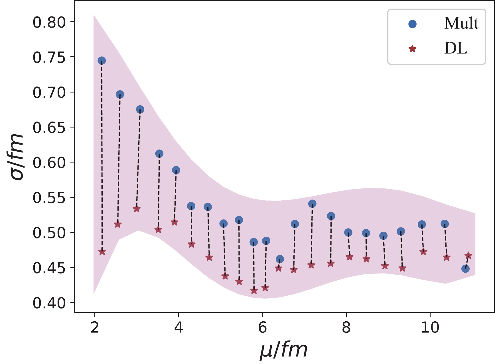
Figure 10. (color online) Comparing the standard deviation of the b distribution obtained using the multiplicity method with that obtained using the CNN. μ is the mean value of the b distribution. 'Mult' denotes the multiplicity method and 'DL' refers to the deep learning method, which is the CNN model here.
-
DL algorithms have revealed a strong capability to construct a map between the input data and target. As a result, we can succeed in various regression or classification tasks without prior knowledge. However, most widely used DL models are not interpretable. Because of their 'complexity' and 'dimensionality', it is difficult to understand how these models work and obtain instructive information from them [39]. Therefore, these DL models are viewed as 'black boxes' in most cases. More effort has been made to open the 'black boxes' of DL algorithms. By analyzing the DNNs on the information plane [40], one can understand the training and learning processes and hence the internal representations of the DNNs [41]. In addition, for CNNs, which are usually used in visual recognition tasks, there have been a number of studies aimed at visualizing them. By operating global average pooling and defining a quantity measuring the importance of neurons in a CNN, one can generate a class activation map (CAM) [42], with which we can localize the crucial regions of a 2D matrix for a CNN to succeed in classification tasks. Based on the CAM method, R. R. Selvaraju et al. proposed a new CNN interpretation method known as gradient-weighted class activation mapping (Grad-CAM) [43]. Compared with the former method, Grad-CAM can be applied to more types of CNNs and can provide more information about what is learned by the neuron network.
In the CAM method, the class activation map for class c (in our case, c is trivial and can be supressed because we have a regression problem instead of a classification problem) is defined as
$ {M^{c}} $ .$ \begin{equation} M^{c}_{x,y}(A) = \sum\limits_k \omega_k^c f_k(A;x,y). \end{equation} $

(2) Here,
$ f_k(A;x,y) $ represents the activation of unit k in the final convolutional layer at spatial location$ (x,y) $ of input data A, and$ \omega_k^c $ is the weight measuring the importance of unit k for class c. In Grad-CAM,$ \omega_k^c $ is defined as the result of performing global average pooling on the gradient of the score for class c with respect to activations$ f_k $ :$ \begin{equation} \omega_k^c = \frac{1}{Z} \sum\limits_x \sum\limits_y \frac{\partial y^c}{\partial f_k(A; x,y)}, \end{equation} $

(3) where
$ (1/Z)\sum\limits_x \sum\limits_y $ represents the operation of global average pooling. Subsequently, the gradient-weighted class activation map is given as$ \begin{equation} L^c = {\rm ReLU} \left(\sum\limits_k \omega_k^c f^k \right). \end{equation} $

(4) CAM and Grad-CAM have succeeded in classification problems. However, several adjustments are required in the definitions of the maps to apply them to our CNN for regression. When Grad-CAM meets classification tasks, only the regions positively correlated with the class of interest should be preserved. Thus, a ReLU operation is performed on the linear combination of maps. However, for regression problems, both the positively-correlated and negatively-correlated features should be considered. Consequently, we redefine an activation map as the absolute value of the linear combination of maps.
$ \begin{equation} L^c = Abs \left(\sum\limits_k \omega_k^c f^k \right). \end{equation} $

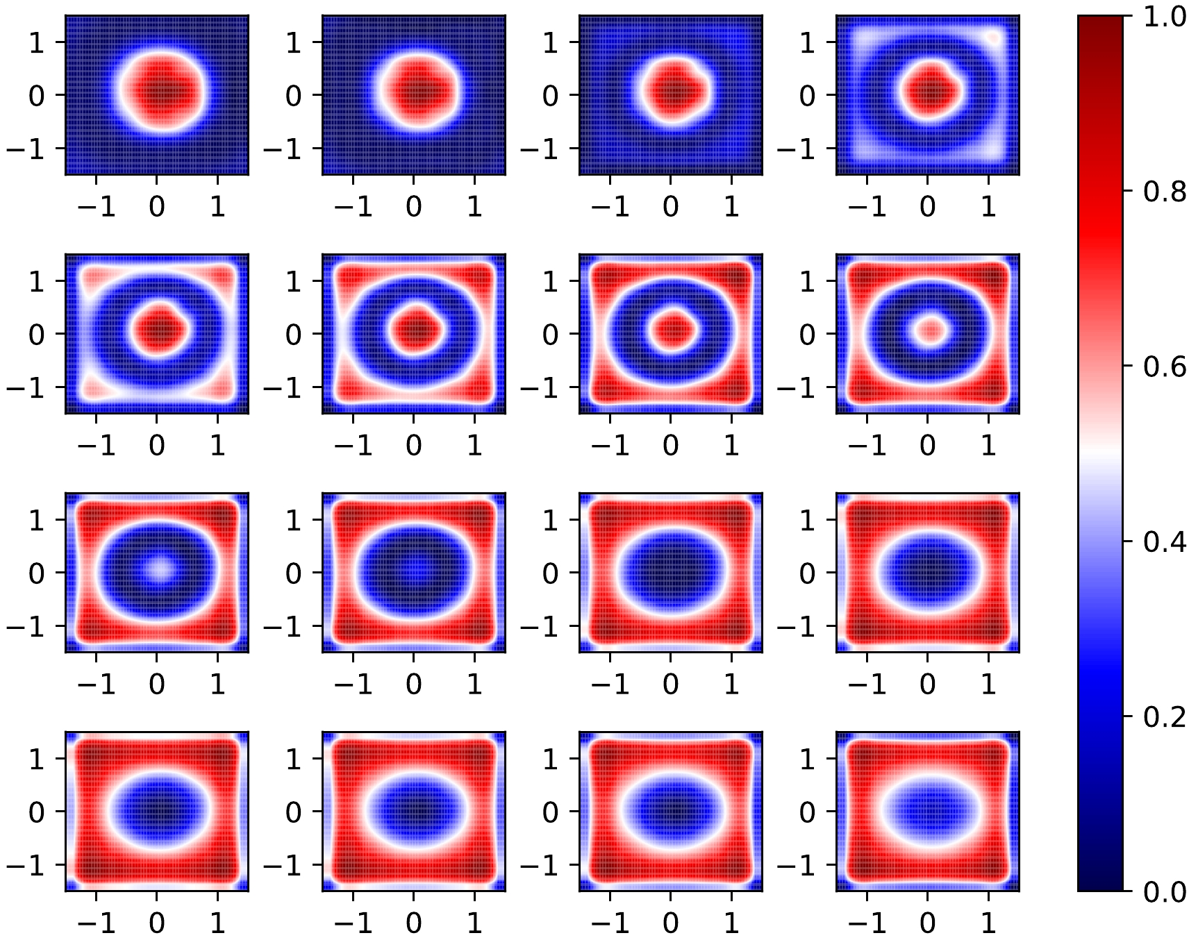
(5) We obtain average 'attention' maps for impact parameters in the interval
$[2,11]$ fm, where our CNN behaves well in prediction (see Fig. 11). It turns out that compared with the cases of central collision, the CNN turns its 'attention' to regions of larger transverse momenta for peripheral collisions. The CNN gives high marks to charged particles with small transverse momenta when it tries to 'recognize' a central event's impact parameter. With an increase in b, the peripheral area of the energy spectrum begins to attract the CNN's attention and becomes more important for distinguishing peripheral events from central ones. This suggests that the CNN focuses on particles with larger transverse momenta for peripheral events. -
In this paper, we investigate the feasibility of applying the DL method to determine a single event's impact parameter in relativistic heavy-ion collisions. By constructing DNN (a MLP) and CNN models, we establish a map between the energy spectrum of final-state charged particles and the impact parameter for a single collision event.
Simulated using the AMPT model, 180000 events of an Au + Au collision at
$ \sqrt{s_{NN}} = 200\ {\rm GeV} $ are generated to train the DL models. In addition, the validation dataset contains 72000 events, which aims at measuring the performance of the DL models. After selecting the best of the trained models, 20000 events are used to test its prediction accuracy. The MLP and CNN models both exhibit high accuracy in the cases of semi-central and semi-peripheral collisions, that is, with an impact parameter of$ 2-10 $ fm. The mean prediction error of the CNN model for events with$ 2 \leq b \leq 11 $ fm ranges from -0.06 to 0.05 fm, and that of the MLP model ranges from -0.08 to 0.08 fm. The mean absolute prediction error on the b interval$ [2, 12.5] $ fm is 0.40${\rm fm} $ for the CNN model. However, these two DL models operate worse for central and peripheral collisions.To investigate the influence of beam energy in this task, we also apply these two DL models with the same architectures to the cases of
$ \sqrt{s_{NN}} = 7.7,\ 39.0,\ 62.4,\ 130.0 $ . The DL models turn out to be effective for both low-energy and high-energy collisions. By extending the pseudorapidity cut, the performance of the CNN is improved, and it reconstructs the impact parameter satisfying$ 2 \leq b \leq 12.5 $ fm with a mean absolute error of 0.35 fm. Subsequently, we propose a scheme to compare the uncertainty on b determination using the multiplicity method with the CNN method. We find that the charged-particle energy spectrum is a better observable than the multiplicity to realize this type of impact parameter determination.By modifying the Grad-CAM algorithm for classification tasks to that available for regression tasks, we obtain 'attention' maps for the CNN model. When meeting central collisions, the CNN has a tendency to focus on particles with small transverse momenta and vice versa for peripheral events.
-
We acknowledge useful discussions with W. B. He, L. G. Pang, X. N. Wang, and K. Zhou.
Determination of the impact parameter in high-energy heavy-ion collisions via deep learning
- Received Date: 2022-03-17
- Available Online: 2022-07-15
Abstract: In this study, Au+Au collisions with an impact parameter of


 Abstract
 HTML
HTML Reference
 Related
 PDF
PDF




 DownLoad: