


 Abstract
 HTML
HTML Reference
 Related
 PDF
PDF


-
Theoretical calculations using the lattice quantum chromodynamics (LQCD) approach reveal that the quark-gluon plasma (QGP) phase, which is chirally restored and color deconfined, is formed at critical conditions of high energy density (
$ \epsilon \sim 1 $ GeV/$\rm{fm}^3$ ) and temperature ($ T \sim 154 $ MeV) [1, 2]. These conditions are expected in ultra-relativistic heavy ion collisions, where a dense medium of quarks and gluons is produced, which then experience rapid-collective expansion before the partons hadronize and subsequently decouple [2]. Numerous experiments are committed to discovering QGP signals assuming quick thermalization, such as the Large Hadron Collider (LHC) at CERN, Geneva, and the Relativistic Heavy Ion Collider (RHIC) at BNL, USA [3, 4]. Regrettably, measurements are limited to final state particles, the majority of which are hadrons [2]; the ensuing transverse and longitudinal expansion of the produced QGP is studied using relativistic viscous hydrodynamics models [5]. In this case, the net entropy, which is essentially conserved from preliminary thermalization until freeze-out [2–5], is an intriguing quantity that may provide significant information on the produced matter during the early stages of nuclear collisions. By accurately accounting for entropy production at various phases of collisions, the observable particle multiplicities in the final state can be linked to system parameters, such as initial temperature, at earlier stages of nuclear collisions [3].Two alternative methods are typically used to calculate the net created entropy during the collisions [3]. Pal and Pratt pioneered the first approach, which calculates entropy using the transverse momentum spectra of various particle species and their source sizes, as calculated using Hanbury Brown-Twiss (HBT) correlations [2, 3]. The original research analyzed experimental data taken from
$ \sqrt{s_{NN}} = 130 $ GeV produced from Au-Au collisions and is still used to determine entropy at various energies [3, 4]. The second approach [6, 7] converts the multiplicity per rapidity$ {\rm d}N/{\rm d}y $ produced in the final state to entropy per rapidity$ {\rm d}S/{\rm d}y $ using the entropy per hadron derived in a hadron resonance gas (HRG) model. Despite the fact that estimating the entropy per rapidity$ {\rm d}S/{\rm d} y $ from the measured multiplicity$ {\rm d}N {ch} /{\rm d}\eta $ is reasonably simple, the conversion factor between the measured charged-particle multiplicity dNch /d and the entropy per rapidity$ {\rm d} S/{\rm d} y $ in literature [7–10] is varied. Hanus and Reygers [3] estimated the entropy production using the transverse momentum distribution from data produced in p-p and Pb-Pb collisions at$ \sqrt{s} = 7 $ , and$ 2.76 $ TeV, respectively, for various particles.Our study aims to calculate the entropy per rapidity
$ {\rm d} S/{\rm d} y $ based on the transverse momentum distribution measured in Pb-Pb collisions at$ \sqrt{s} = 2.76 $ and$ 5.02 $ TeV for particles π, k, p, Λ, Ω, and$ \bar{\Sigma} $ and π, k, p, Λ, and$ K_s^0 $ , respectively. For a precise estimation of the entropy per rapidity$ {\rm d} S/{\rm d} y $ , we fit the transverse momentum distribution of the considered particles using two thermal approaches, the Tsalis distribution [11, 12] and the HRG model [13]. This enables us to cover a large range of the measured transverse particle momentum$ p_{\rm T} $ , up to$ \sim 20 $ GeV/c (unlike Hanus, who used a small range of$ p_{\rm T} $ $ \sim 1.5 $ GeV/c), and consider the particle's mass as a free parameter. Indeed, we use the exact value of the particle's mass for all considered particles as in the Particle Data Group (PDG) [14]. The Tsallis distribution succeeds in describing a large range of$ p_{\rm T} $ but cannot describe its entire range. That is why we use the HRG model to fit the other part of$ p_{\rm T} $ . Moreover, we estimate the entropy per rapidity$ {\rm d} S/{\rm d} y $ for the considered particles using a highly promising simulation model, the artificial neural network (ANN). Recently, several modeling methods based on soft computing systems have included the application of artificial intelligence (AI) techniques. These evolution algorithms have a physically powerful existence in this field [15–19]. The behavior of p-p and Pb-Pb interactions are complicated owing to the non-linear relationship between the interaction parameters and the output. Understanding the interactions of fundamental particles requires multi-part data analysis, and AI techniques are vital. These techniques are useful as alternative approaches to conventional techniques [20]. In this sense, AI techniques such as ANNs, genetic algorithms (GAs), genetic programming (GP), and genetic expression programming (GEP) can be used as alternative tools to simulate these interactions [15, 19]. The motivation for using an ANN approach is its learning algorithm, which learns the relationships between variables in datasets and then creates models to explain these relationships (mathematically dependent) [21]. There is a desire for fresh computer science methods to analyze experimental data for a better understanding of various physics phenomena. ANNs have gained popularity in recent years as a powerful tool for establishing data correlations and have been successfully employed in materials science owing to its generalization, noise tolerance, and fault tolerance [22]. This enables us to use it to estimate the entropy per rapidity$ {\rm d}S/{\rm d}y $ . The results are then compared to available experimental data and the results obtained from previous calculations.This paper is organized as follows: In Sec. II, the approaches used in this study are presented, the results and discussion are shown in Sec. III, and the conclusion is presented in Sec. IV. A mathematical description of the entropy per rapidity
$ {\rm d}S/{\rm d}y $ and the transverse momentum spectra based on both the Tsallis distribution and HRG model are given in the Appendices. -
In Sec. II, we discuss the methods used to estimate the entropy per rapidity
$ {\rm d}S/{\rm d}y $ for various particles. The first method depends on the measured spectra of the considered particles [3]. In the second, we use the ANN model, which may be considered the future simulation model [22]. -
Here, we review the entropy per rapidity
${\rm d}S/{\rm d}y $ estimation from the phase space function distribution calculated using particle distribution spectra and femtoscopy [3]. The fundamentals of this approach are shown in Ref. [3, 23, 24].For any particle species in the thermal freeze-out stage, the entropy S is obtained from the phase space distribution function
$ f (\vec{p},\vec{r}) $ [3].$ \begin{equation} S=(2 J+1) \int \frac{{\rm d}^{3} r {\rm d}^{3} p}{(2 \pi)^{3}}[-f \ln f \pm(1 \pm f) \ln (1 \pm f)], \end{equation} $

(1) where
$ + $ and$ - $ represent bosons and fermions, respectively. The quantity$ 2 J + 1 $ represents the spin degeneracy of particles. The net entropy produced in nuclear collisions is then obtained by summing all the entropy of the created hadrons species. From Eq. (1), the integral can be expressed in a series expansion form$ \begin{equation} \pm(1 \pm f) \ln (1 \pm f)=f \pm \frac{f^{2}}{2}-\frac{f^{3}}{6} \pm \frac{f^{4}}{12}+\ldots, \end{equation} $

(2) The source radii, observed from HBT two particle correlations [25] in three dimensions, are calculated from a longitudinally co-moving system (LCMS) where the pair momentum component along the direction of the beam vanishes. In the LCMS, the density function of the source is parametrized by a Gaussian in three dimension, allowing the phase space distribution function to be represented as [3]
$ \begin{equation} f(\vec{p}, \vec{r})=\mathcal{F}(\vec{p}) \exp \left(-\frac{x_{\mathrm{out}}^{2}}{2 R_{\mathrm{out}}^{2}}-\frac{x_{\rm {side }}^{2}}{2 R_{\rm {side }}^{2}}-\frac{x_{\rm {long }}^{2}}{2 R_{\rm {long }}^{2}}\right), \end{equation} $

(3) where
$ \mathcal{F}(\vec{p}) $ , the maximum phase density, is given by [2, 3]$ \begin{equation} \mathcal{F}(\vec{p})=\frac{(2 \pi)^{3 / 2}}{2 J+1} \frac{{\rm d}^{3} N}{{\rm d}^{3} p} \frac{1}{R_{\rm {out }} R_{\rm {side }} R_{\rm {long }}}. \end{equation} $

(4) In Eqs. (3) and (4), the source radii are expressed in terms of the momentum
$ \vec{p} $ .Owing to restricted statistics, in many circumstances, only the source radius
$ R_{\mathrm{inv}} $ measured in one dimension, which is computed in the pair rest frame (PRF), may be obtained experimentally.The relationship between the PRF's
$ R_{\mathrm{inv}} $ and the three-dimensional source radii in the LCMS is considered as [2, 3]$ \begin{equation} R_{\mathrm{inv}}^{3} \approx \gamma R_{\mathrm{out}} R_{\mathrm{side}} R_{\mathrm{long}}, \end{equation} $

(5) where
$ \gamma=m_{\mathrm{T}} / m \equiv \sqrt{m^{2}+p_{\mathrm{T}}^{2}} / m. $ In Refs. [3, 26], the ALICE collaboration published values for both
$ R_{\mathrm{inv}} $ and$ R_{\mathrm{out}}, \; R_{\rm {side }},\; R_{\rm {long }} $ , which were determined from two pion correlations in Pb-Pb nuclear collisions at$\sqrt{s_{NN}}=2.76 \;\mathrm{TeV}$ .From these data, Hanus et al. expressed a more general formula for Eq. (5) as [3]
$ \begin{equation} R_{\rm {inv }}^{3} \approx h(\gamma) R_{\rm {out }} R_{\rm {side }} R_{\rm {long }}, \end{equation} $

(6) with
$ h(\gamma)=\alpha \gamma^{\beta} $ .From Eq. (5), the entropy per rapidity
$ {\rm d} s/ {\rm d} y $ can be given as [3]$ \begin{aligned}[b] \frac{{\rm d} S}{{\rm d} y}=& \int {\rm d} p_{\rm T} 2 \pi p_{\rm T} E \frac{{\rm d}^{3} N}{{\rm d}^{3} p}\left(\frac{5}{2}-\ln \mathcal{F} \pm \frac{\mathcal{F}}{2^{5 / 2}}\right.\\ &\left.-\frac{\mathcal{F}^{2}}{2 \times 3^{5 / 2}} \pm \frac{\mathcal{F}^{3}}{3 \times 4^{5 / 2}}\right), \end{aligned} $

(7) where
$ \mathcal{F} $ , the phase space distribution function, is given by [3]$ \begin{equation} \mathcal{F}=\frac{1}{m} \frac{(2 \pi)^{3 / 2}}{2 J+1} \frac{1}{R_{\mathrm{inv}}^{3}\left(m_{\mathrm{T}}\right)} E \frac{{\rm d}^{3} N}{{\rm d}^{3} p}. \end{equation} $

(8) For a better description of central Pb-Pb, Hanus et al. approximated the expression
$ (1+f) \ln (1+f) $ in terms of Eq. (1) with numerical coefficients$ a_{i} $ , which is also used for high multiplicity values of$ \mathcal{F} $ as [3]$ \begin{equation} \frac{{\rm d} S}{{\rm d} y}=\int {\rm d} p_{T} 2 \pi p_{\rm T} E \frac{{\rm d}^{3} N}{{\rm d}^{3} p}\left(\frac{5}{2}-\ln \mathcal{F}+\sum_{i=0}^{7} a_{i} \mathcal{F}^{i}\right). \end{equation} $

(9) To calculate the entropy per rapidity
$ {\rm d} S/{\rm d} y $ for the considered hadrons, the measured spectra of the transverse momentum$ E ({{\rm d}^{3} N}/{{\rm d}^{3} p}) $ must be extrapolated at$ p_{\rm T} = 0 $ . To achieve this, we compare the$ p_{\rm T} $ momentum spectra to two various fitting functions estimated from two well-known models, the Tsallis distribution and HRG model. A mathematical description of the transverse momentum distribution$ E ({{\rm d}^{3} N}/{{\rm d}^{3} p}) $ using the HRG model and Tsallis distribution is given in Appendices B and C, respectively. -
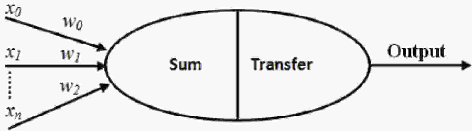
The ANN model [27–33] is a machine learning technique most popular in the high-energy physics community. In the last decade, important physics results have been separated using this model. A neuron is an essential processing component of the ANN model (see Fig. 1), which forms a weighted sum of its input and passes the outcome to the yield through a non-linear transfer function. These transfer functions can also be linear, and then the weighted sum is sent directly in the output direction. Eqs. (10) and (11) represent the weighted summation of the inputs and the non linear transfer function to the output of the neuron, respectively.
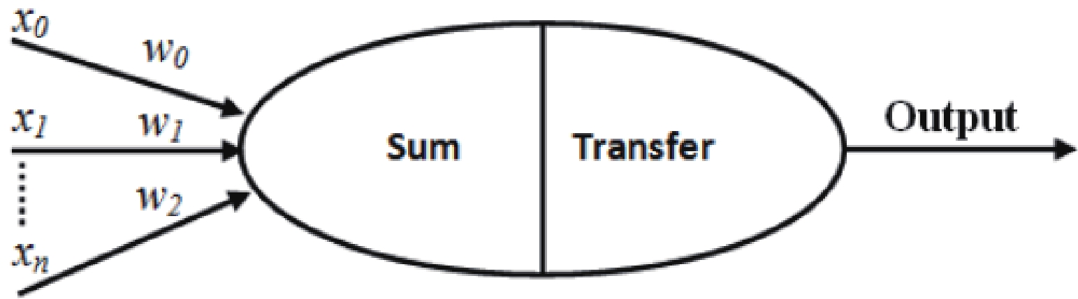
Figure 1. Schematic diagram of a basic formal neuron.
$ \begin{equation} \sigma=\sum\limits_{n} x_{n} w_{n}, \end{equation} $

(10) $ \begin{equation} Y=f(\sigma). \end{equation} $

(11) The most widely recognized ANN is the multilayer feed forward neural network dependent on the backpropagation (BP) learning algorithm. Backpropagation learning calculation is the most incredible of the multi-layer calculations, as revealed in Alsmadi et al., [34]. The multilayer feed-forward ANN structure is a blend of various layers (see Fig. 2). The primary layer (input layer) is the information layer, which presents the experimental data that is then prepared and spread to the yield layer (output layer) through at least one hidden layer.
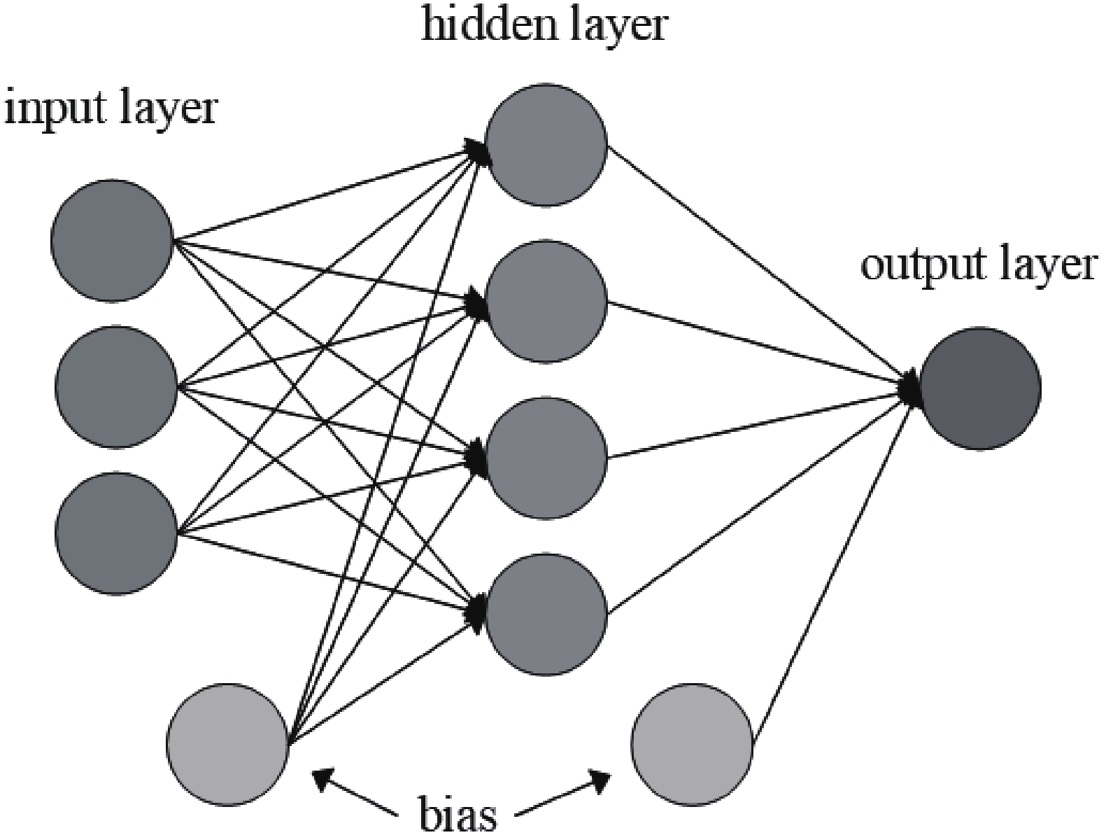
Figure 2. Representative architecture of a feed-forward artificial neural network.
The number of hidden layers and neurons required in every hidden layer is important when designing a network. The best number of neurons and hidden layers relies on factors such as the number of inputs, output of the network, commotion of the target data, intricacy of the error function, network design, and network training algorithm. In most cases, it is basically impossible to effortlessly decide the ideal number of hidden layers and neurons in each hidden layer without training the network. The training network involves constantly adjusting the weights of the association links between the processing of input patterns and the required output components relating to the network. A block diagram of the backpropagation network is shown in Fig. 3. The aim of training is to reduce and minimize the error representing the difference between the output experimental data
$ (t) $ and simulation results$ (y) $ to accomplish the most ideal result.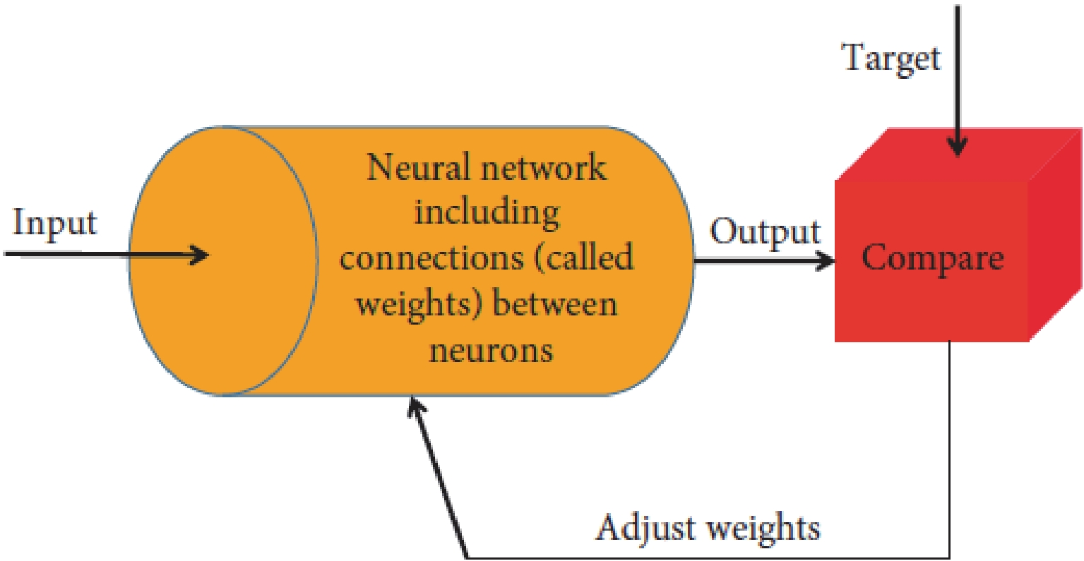
Figure 3. (color online) Back-propagation network block diagram.
Thus, the next mean square error (MSE) should be minimized [35].
$ \begin{equation} MSE=\frac{1}{n} \sum\limits_{i=1}^{n}\left(t_{i}-y_{i}\right)^{2}, \end{equation} $

(12) where n is the number of data points used to train the model.
In this study, the data are divided into three parts: the training set (
$ 70 $ %), test set ($ 15 $ %), and validation set ($ 15 $ %). The aim of this classification is to ensure the validation of the used ANN model after training by testing it to predict random values of the used data. A detailed description of the training algorithm is shown in Appendix E. -
In this section, we discuss the obtained results of the entropy per rapidity
$ {\rm d}S/{\rm d}y $ for central Pb-Pb at LHC energies$ \sqrt{s} =2.76 $ and$ 5.02 $ TeV. The ANN simulation model is also used to estimate the entropy per rapidity$ {\rm d}S/{\rm d}y $ at the considered energies. First, we train the ANN model to fit 70% of the used experimental data for the particle spectra of the mentioned particles. Then, we check the validation of the model by testing it to predict some values of the available experimental data of these particles. A comparison between the simulated results obtained from the experimental measurements and the simulated results is also shown. -
We calculate the entropy per rapidity
$ {\rm d}S/{\rm d}y $ for particles π, k, p, Λ, Ω, and$ \bar{\Sigma} $ produced in central Pb-Pb collisions at$ \sqrt{s} =2.76 $ TeV. The obtained results are compared to those estimated using the ANN simulation model and those calculated in [3]. As the experimental input, the computation includes the transverse momentum spectra of particles π, k, p [36], Λ [37], Ω, and$ \bar{\Sigma} $ [38]. Furthermore, we employ the ALICE-measured HBT radii to calculate the particle spectra of the mentioned particles [39]. The Rprop based ANN is used to simulate$ p_T $ spectra for the same particles. This procedure involves a supervised learning algorithm that is implemented using a set of input-output experimental data. Because the nature of the output (various particles) is not the same, authors chose individual neural systems trained independently. Six networks are chosen to simulate experimental data according to six different particles. Our networks have three inputs and one output. The inputs are$ \sqrt{s} $ ,$ P_{\rm T} $ , and centrality. The output is$ \dfrac{1}{N_{\rm evt} }\dfrac{{\rm d}^2 N}{{\rm d} y {\rm d} p_{\rm T}} $ .Number of layers between the input and output (hidden layer) and the number of neurons in the hidden layer is selected by trial and error. In the beginning, we start with one hidden layer and one neuron in the hidden layer. Then, the number of hidden layers and neurons increase regularly. By changing the number of neurons, the performance of the network changes. The learning performance of the network can be measured and evaluated by inspecting the coefficients of the MSE and regression value (R) for the training, test, and validation sets. If the coefficient of the MSE is close to zero, the difference between the network and desired output is small. Moreover, if this value is zero, there is no difference or no error. However, R determines the correlation level of the output. If its value is equal to
$ 1 $ , the experimental results are compared with the ANN model output, and a very good agreement has been found between them. In our study, the best MSE and R values are obtained using one hidden layer. The number of neurons in the hidden layer is ($ 10 $ ), ($ 10 $ ), ($ 5 $ ), ($ 10 $ ), ($ 8 $ ), and ($ 7 $ ) for particles π, k, p, Λ, Ω, and$ \bar{\Sigma} $ , respectively. A simplification of the proposed ANN networks are shown in Fig. 4 for particles π (a), k (b), p (c), Λ(d), Ω(e), and$ \bar{\Sigma} $ (f).
Figure 4. (color online) Schematic diagram of the basic formal neuron network for particles (a) π, (b) k, (c) p, (d) Λ, (e) Ω, and (f)
$ \bar{\Sigma} $ .The generated MSE and R values for the training, test, and validation sets are shown in Figs. 5 and 6 for particles π (a), k (b), p (c), Λ (d), Ω (e), and
$ \bar{\Sigma} $ (f). The MSE and R values are summarized in Table 1 after epoch$ 77 $ ,$ 8 $ ,$ 11 $ ,$ 10 $ ,$ 11 $ , and$ 16 $ for particles π (a), k (b), p (c), Λ (d), Ω (e), and$ \bar{\Sigma} $ (f). In all cases, the R values are closed to one. The MSE and regression values indicate good agreement between the ANN results and experimental data.ANN parameters Particles π K p Λ Ω $ \bar{\Sigma} $ 

Inputs $ \sqrt{S} $ 

$ p_{\rm T}/\mathrm{GeV} $ 

Centrality $ \sqrt{s} $ 

$2.76/\mathrm{TeV}$ 

Output $ \dfrac{1}{N_{\rm evt} }\dfrac{{\rm d}^2 N}{ {\rm d} y {\rm d} p_{\rm T}} $ 

Hidden layers 1 Neurons $ 10 $ 

$ 10 $ 

$ 5 $ 

$ 10 $ 

$ 8 $ 

$ 7 $ 

Epochs $ 77 $ 

$ 8 $ 

$ 11 $ 

$ 10 $ 

$ 11 $ 

$ 16 $ 

MSE (Training) $ 8.325 $ 

$ 1.85178 \times 10^{-2} $ 

$ 1.67861 \times 10^{-3} $ 

$ 1.97367 \times 10^{-2} $ 

$ 1.93485 \times 10^{-9} $ 

$ 2.75711 \times 10^{-6} $ 

MSE (Test) $ 9.05709 $ 

$ 2.6585 $ 

$ 9.57606 \times 10^{-3} $ 

$ 6.73839 \times 10^{-2} $ 

$ 3.4253 \times 10^{-6} $ 

$ 1.26585 \times 10^{-4} $ 

MSE (Validation) $ 0.012662 $ 

$ 0.41663 $ 

$ 0.0018642 $ 

$ 0.0072329 $ 

$ 1.4303 \times 10^{-8} $ 

$ 2.3812 \times 10^{-5} $ 

R (Training) $ 0.99997 $ 

$ 0.99991 $ 

$ 0.99987 $ 

$ 0.99426 $ 

$ 1 $ 

$ 0.99986 $ 

R (Test) $ 0.9976 $ 

$ 0.9999 $ 

$ 0.99995 $ 

$ 0.99995 $ 

$ 1 $ 

$ 0.99944 $ 

R (Validation) $ 1 $ 

$ 0.99201 $ 

$ 0.99981 $ 

$ 0.99771 $ 

$ 1 $ 

$ 0.99997 $ 

Training algorithms Rprop Training functions trainrp Transfer functions of hidden layer tansig tansig tansig tansig tansig tansig Output functions Purelin Table 1. ANN parameters for particles π, k, p, Λ, Ω, and
$ \bar{\Sigma} $ at$ \sqrt{s} =2.76 $ TeV.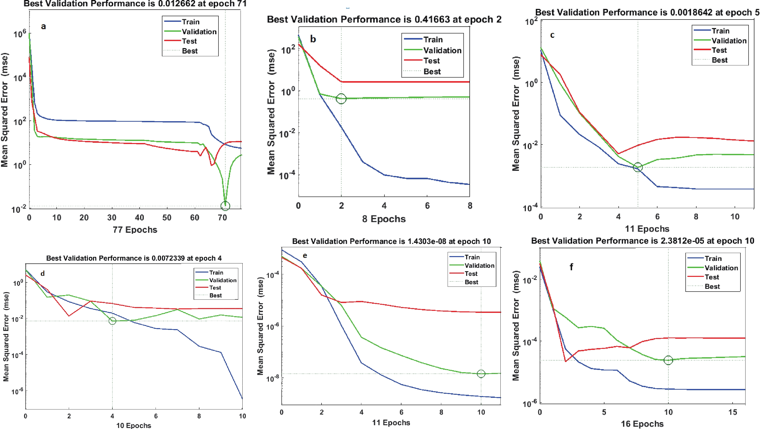
Figure 5. (color online) Best training, validation, and test performance (MSE) for particles (a) π, (b) k, (c) p, (d) Λ, (e) Ω, and (f)
$ \bar{\Sigma} $ .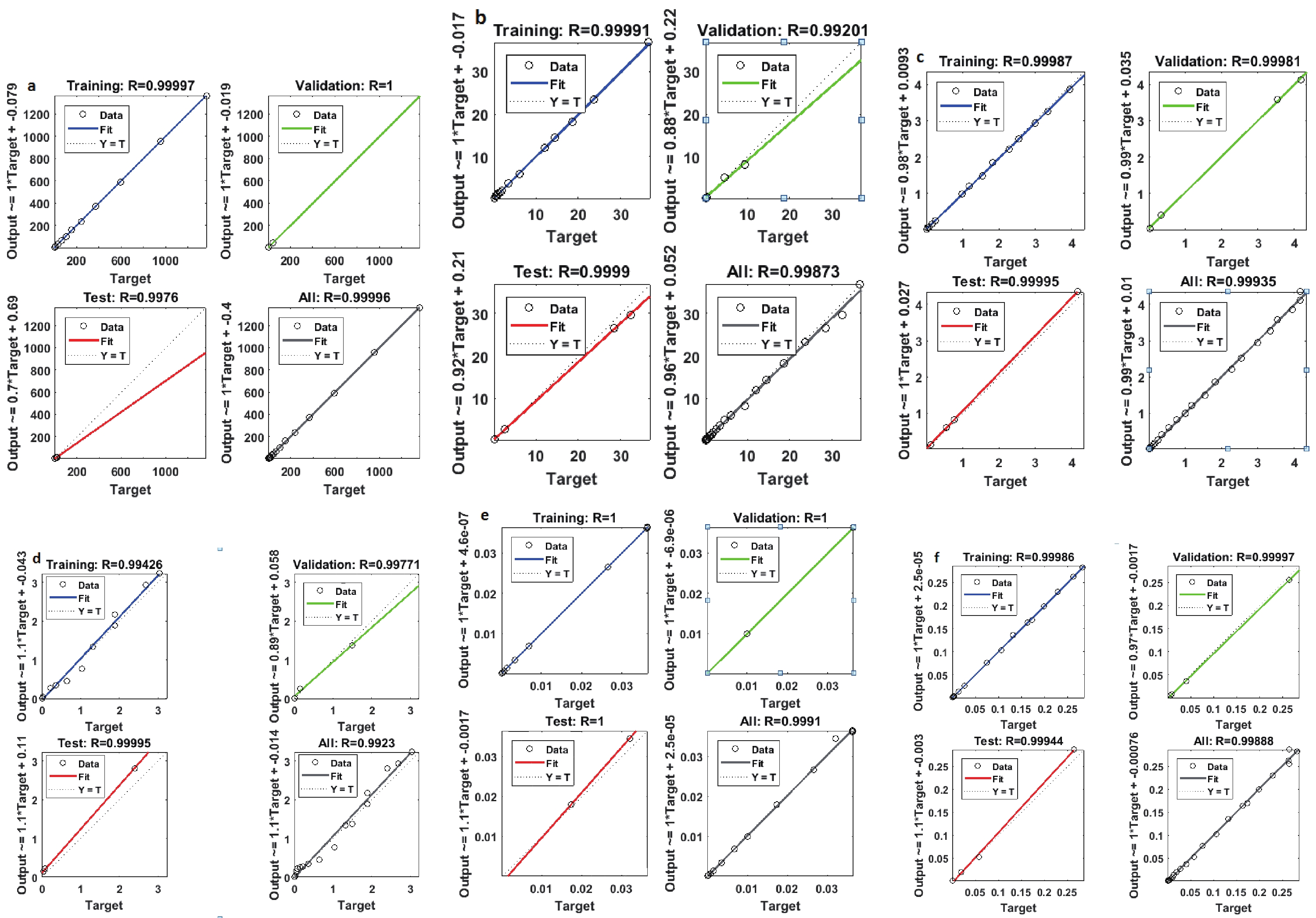
Figure 6. (color online) Regression values (R) for the training, validation, and test sets for particles (a) π, (b) k, (c) p, (d) Λ, (e) Ω, and (f)
$ \bar{\Sigma} $ at the used epoch.The transfer function used in the hidden layer is tansig for all particles and purelin for the output layer. All parameters used in the ANN model are represented in Table 1.
To estimate the entropy S, extrapolation of the observed transverse momentum spectra to
$ p_{\rm T} = 0 $ is required. To achieve this, we fit both the experimental and simulated$ p_{\rm T} $ spectra to two various functional models, the Tsallis distribution [11, 12] and HRG model [13]. The aim of using two different models is to fit the entire$ p_{\rm T} $ curve.Figure 7 shows the particle spectrum measured by the ALICE collaboration [40], which is represented by closed blue circles and fitted to the Tasllis distribution [11, 12], represented by the solid red curve, to extrapolate the spectrum at
$ p_{\rm T} = 0 $ . The HBT one-dimensional radii are scaled by$ ((2 + \gamma)/3)^{1/2} $ [3, 40] to become a function of transverse mass,$ m_{\rm T} $ . A comparison of the experimental and simulated particle spectra$ p_{\rm T} $ to both the Tsallis distribution and HRG model is shown in Fig. 8 for particles π (a), k (b), p (c), Λ (d), Ω (e), and$ \bar{\Sigma} $ (f). It is clear from Fig. 8 that the use of various forms of the fitting function is suitable because the Tsallis function can only fit the left side of the$ p_{\rm T} $ curve at$ 0.001 < y < 6 $ , while the HRG model can fit the right side$ 6 < y < 12 $ as well. The obtained fitting parameters as a result of both the Tsallis distribution and HRG model are summarized in Tables 2 and 3, respectively.Particle Tsallis distribution HRG model $ \chi^{2} $ /dof

dN/dy $ T_{Ts} $ /GeV

q V/ $ {\rm fm}^3 $ 

$ T_{\rm th} $ /GeV

μ/GeV π $ 739.886 $ 

$ 0.0658 $ 

$ 1.2305 $ 

$ 3.41332 \times 10^1 \pm 6.103 $ 

$ 3.3881\times 10^{-1} \pm 4.8231 \times 10^{-3} $ 

$ 1.2549 \pm 4.219 \times 10^{-2} $ 

$ 13.6/12 $ 

K $ 88.3303 $ 

$ 0.1711 $ 

$ 1.1132 $ 

$ 1.38260 \times 10^1 \pm 3.6055 $ 

$ 3.13028\times 10^{-1} \pm 4.36637\times 10^{-3} $ 

$ 1.26516 \pm 6.32063\times 10^{-2} $ 

$ 163.536/11 $ 

p $ 39.8814 $ 

$ 0.31752 $ 

$ 1.13739 $ 

$ 5.57340\times 10^2 \pm 3.31936\times 10^{2} $ 

$ 3.89646\times 10^{-1}\pm 1.79383\times 10^{-3} $ 

$ 3.10152\times 10^{-2} \pm 2.39531\times 10^{-1} $ 

$ 25.3567/12 $ 

Λ $ 47.6767 $ 

$ 0.4388 $ 

$ 1.1148 $ 

$ 48.7847 \pm 48983.2 $ 

$ 0.503582 \pm 45.8599 $ 

$ 1.12747 \pm 626.183 $ 

$ 286.085/15 $ 

Ω $ 1.24793 $ 

$ 0.4277 $ 

$ 1.14736 $ 

$ 1.24168 \pm 1.0661 $ 

$ 0.539524 \pm 0.0513 $ 

$ 1.14468 \pm 0.3706 $ 

$ 0.0199/7 $ 

$ \bar{\Sigma} $ 

$ 6.5279 $ 

$ 0.4640 $ 

$ 1.1245 $ 

$ 4.38896 \pm 1.5158 $ 

$ 0.545919 \pm 0.0209 $ 

$ 0.865 \pm 0.1993 $ 

$ 3.0475/15 $ 

Particle Tsallis distribution HRG model $ \chi^{2} $ /dof

${\rm d}N /{\rm{d}}y$ 

T/GeV q V/ $ {\rm fm}^3 $ 

T/GeV μ/GeV π $ 775.496 $ 

$ 0.08174 $ 

$ 1.1873 $ 

$ 23.5314 \pm 15.5048 $ 

$ 0.3286 \pm 0.0448 $ 

$ 1.3797 \pm 0.09944 $ 

$ 32.0297/11 $ 

K $ 88.2811 $ 

$ 0.1719 $ 

$ 1.111 $ 

$ 13.8111 \pm 1.993 $ 

$ 0.3125 \pm 0.00478 $ 

$ 1.2664 \pm 0.0292 $ 

$ 159.234/11 $ 

p $ 40.2232 $ 

$ 0.31542 $ 

$ 1.14088 $ 

$ 26.0248 \pm 3.2175 $ 

$ 0.3758 \pm 0.0053 $ 

$ 1.2924 \pm 0.0486 $ 

$ 23.8924/12 $ 

Λ $ 47.953 $ 

$ 0.4458 $ 

$ 1.11257 $ 

$ 50.852 \pm 54211.8 $ 

$ 0.5057 \pm 30.6755 $ 

$ 1.1584 \pm 358.797 $ 

$ 285.464/15 $ 

Ω $ 1.2580 $ 

$ 0.4125 $ 

$ 1.1492 $ 

$ 1.17248 \pm 0.294 $ 

$ 0.6464 \pm 0.0184 $ 

$ 0.4864 \pm 0.1411 $ 

$ 0.02487/7 $ 

$ \bar{\Sigma} $ 

$ 6.5309 $ 

$ 0.4595 $ 

$ 1.1260 $ 

$ 4.3795 \pm 1.8017 $ 

$ 0.5577 \pm 0.0248 $ 

$ 0.7849 \pm 0.2178 $ 

$ 3.1109/15 $ 

Table 3. Same as in Table 2, but the statistical fit results, from both used models, are compared to those of the ANN simulation model.
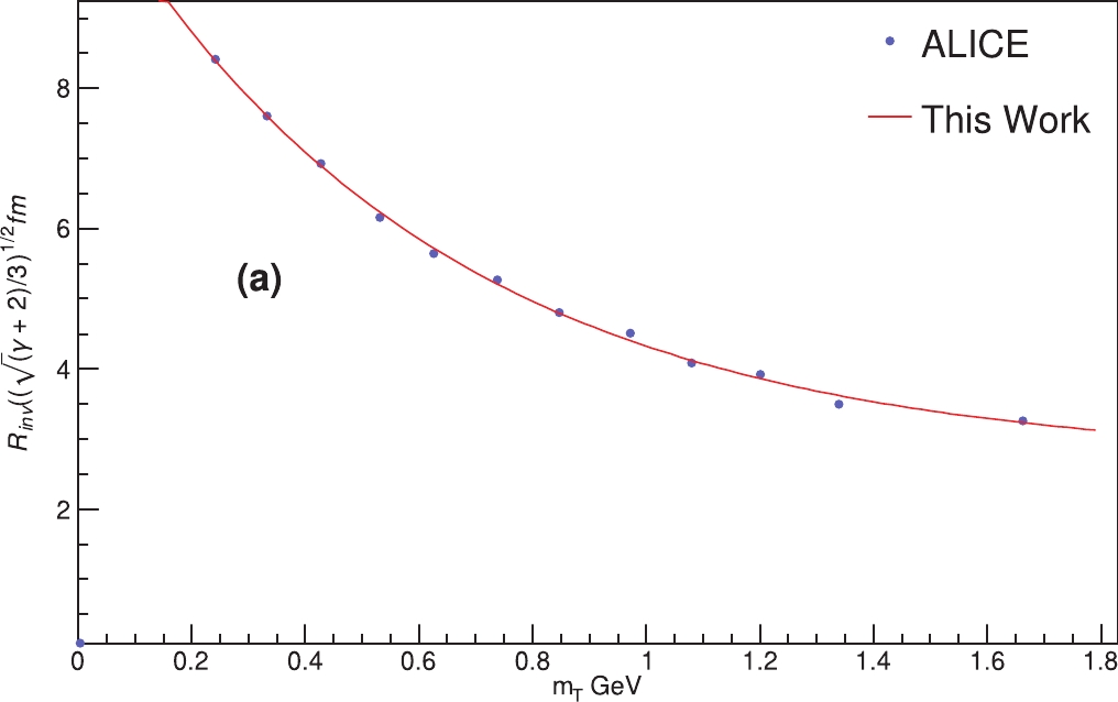
Figure 7. (color online) Particle spectrum measured by the ALICE collaboration [40], represented by blue closed circles, is fitted to the Tsallis distribution [11, 12], which is represented by the solid red curve, to extrapolate the spectrum at
$ p_{\rm T} = 0 $ . The HBT one-dimensional radii are scaled by$ ((2 + \gamma)/3)^{1/2} $ [3, 40] to become a function of transverse mass,$ m_{\rm T} $ .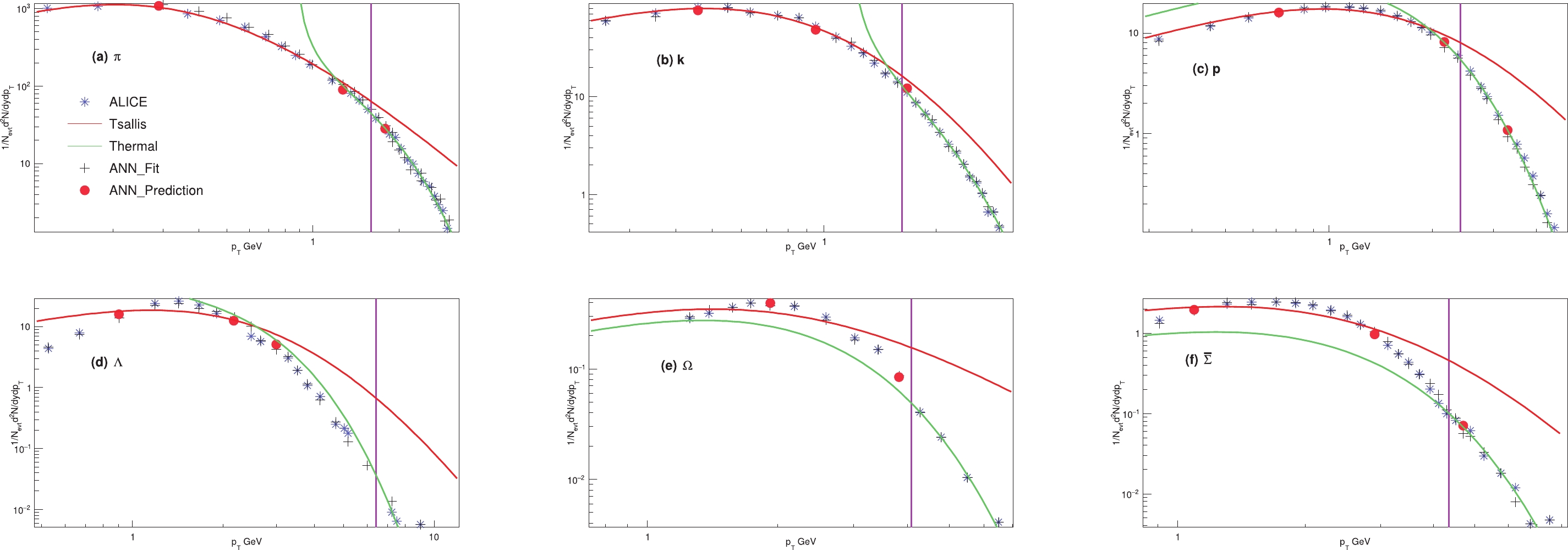
Figure 8. (color online) Transverse momentum distribution measured by the ALICE experiment collaboration [36–38] at a centre of mass energy
$ = 2.76 $ TeV, which is represented by blue open circles for particles π (a), k (b), p (c), Λ (d), Ω (e), and$ \bar{\Sigma} $ (f), is compared to the statistical fits from the Tsallis distribution, which has perfect fits at$ 0.001 < y < 6 $ and is represented by red solid lines, given by Eq. (40), and the HRG model, which works in$ 6 < y < 12 $ and is represented by green solid lines, given by Eq. (35). A border line is drawn between the Tsallis and HRG models, shown in purple. The experimental data and the results of both models are then compared to that obtained from the ANN simulation model, represented by dark brown plus signs. The prediction of the ANN model is presented by red closed circles.The function that describes the non-linear relationship between the inputs and output based on the ANN simulation model is given in Appendix D. The results of the ANN simulation (training and testing), Tsallis distribution, and HRG model of the particle spectra for the suggested particles compared with experimental data are shown in Fig. 8. The estimated entropy per rapidity
$ {\rm d}S/{\rm d}y $ from Pb-Pb central collisions at$ \sqrt{s} =2.76 $ TeV using the Tsallis distribution, HRG model, and ANN model for particles π, k, p, Λ, Ω, and$ \bar{\Sigma} $ is represented in Table 4. The effect of both the Tsallis distribution and HRG model fitting functions on the estimated entropy per rapidity$ {\rm d}S/{\rm d}y $ is also shown in Table 4. We compare the entropy per rapidity obtained from the statistical fits (HRG and Tsallis models) and ANN model to that obtained in Ref. [3].Particle $ ({\rm d}S/{\rm d}y)_{y=0} $ 

$ ({\rm d}S/{\rm d}y)_{y=0} $ 

supplemented by Tsallis$ ({\rm d}S/{\rm d}y)_{y=0} $ 

supplemented by HRG model$ ({\rm d}S/{\rm d}y)_{y=0} $ 

estimated by ANN model$ ({\rm d}S/{\rm d}y)_{y=0} $ Ref. [3]

π $ 1908.21 $ 

$ 2260.85 $ 

$ 2267.58 $ 

$ 2265.17 $ 

$ 2182 $ 

K $ 478.351 $ 

$ 512.399 $ 

$ 514.321 $ 

$ 514.347 $ 

$ 605 $ 

p $ 265.648 $ 

$ 278.125 $ 

$ 278.486 $ 

$ 277.937 $ 

$ 266 $ 

Λ $ 304.334 $ 

$ 325.742 $ 

$ 321.939 $ 

$ 300 $ 

$ 320 $ 

Ω $ 10.1561 $ 

$ 14.4025 $ 

$ 14.2159 $ 

$ 13.3129 $ 

$ 16 $ 

$ \bar{\Sigma} $ 

$ 54.3717 $ 

$ 58.3102 $ 

$ 57.8227 $ 

$ 58.1449 $ 

$ 58 $ 

Table 4. Estimated entropy per rapidity
$ {\rm d}S/{\rm d}y $ from Pb-Pb central collisions at$ \sqrt{s} =2.76 $ TeV using the Tsallis distribution, HRG model, and ANN model. The obtained results are compared to that obtained in Ref. [3].As shown in Table 4, the calculated entropy per rapidity
$ {\rm d}S/{\rm d}y $ from the statistical fits (HRG and Tsallis models), ANN model, and Ref. [3] are in agreement. The excellent agreement between the estimated results of$ {\rm d}S/{\rm d}y $ from the ANN simulation model and Ref. [3] encourage us to use it at other energies. -
For central Pb-Pb collisions at
$ \sqrt{s} = 5.02 $ TeV, we calculate the entropy per rapidity$ {\rm d}S/{\rm d}y $ for particles π, k, p, Λ, and$ K_s^0 $ . Transverse momentum spectra of the particles π, k, p [41], Λ, and$ K_s^0 $ [42] are used as the experimental input for the computation. We also employ ALICE measured HBT source radii [39] and use the same deduced inputs for the ANN model. We apply the ANN model to acquire the$ p_{\rm T} $ spectra of the particles π, k, p, Λ, and$ K_s^0 $ according to the input parameters represented in Table 5. First, we train the ANN model to fit ($ 70 $ %) of the used experimental data. Subsequently, we test its validation through ($ 30 $ %) for both test and validation sets to predict some of the values of the experimental data. Five networks are chosen to simulate experimental data according to different particles. The best performance training, test, and validation values R are obtained using one hidden layer. The number of neurons in the hidden layer is ($ 12 $ ), ($ 10 $ ), ($ 14 $ ), ($ 9 $ ), and ($ 7 $ ) for particles π, k, p, Λ, and$ K_s^0 $ , respectively. A simplification of the proposed ANN networks are shown in Fig. 9 for particles (a) π, (b) k, (c) p, (d) Λ, and (e)$ K_s^0 $ .ANN parameters Particles π K p Λ $ k_s^0 $ 

Inputs $ \sqrt{S} $ 

$ P_{\rm T}/\mathrm{GeV}$ 

Centrality $ \sqrt{S} $ 

$ 5.02 $ TeV

Output $ \dfrac{1}{N_{\rm evt} }\dfrac{{\rm d}^2 N}{ {\rm d} y {\rm d} p_{\rm T}} $ 

Hidden layers 1 Neurons $ 12 $ 

$ 10 $ 

$ 14 $ 

$ 9 $ 

$ 7 $ 

Epochs $ 19 $ 

$ 47 $ 

$ 8 $ 

$ 9 $ 

$ 14 $ 

MSE (Training) $ 5.41199 \times 10^{-2} $ 

$ 3.7357 \times 10^{-7} $ 

$ 2.45426 \times 10^{-30} $ 

$ 2.42245 $ 

$ 1.30543 \times 10^{-2} $ 

MSE (Test) $ 5.3254 $ 

$ 1.50092 \times 10^{-6} $ 

$ 5.03187 \times 10^{-2} $ 

$ 1.37346 $ 

$ 4.64693 \times 10^{-1} $ 

MSE (Validation) $ 0.0024821 $ 

$ 1.5046 \times 10^{-7} $ 

$ 0.052807 $ 

$ 0.0042563 $ 

$ 0.49388 $ 

R (Training) $ 0.99979 $ 

$ 1 $ 

$ 1 $ 

$ 0.99205 $ 

$ 0.99995 $ 

R (Test) $ 0.98118 $ 

$ 1 $ 

$ 0.99999 $ 

$ 0.95224 $ 

$ 1 $ 

R (Validation) $ 0.99989 $ 

$ 1 $ 

$ 0.99999 $ 

$ 0.99878 $ 

$ 0.99931 $ 

Training algorithms Rprop Training functions trainrp Transfer functions of hidden layer tansig tansig tansig tansig tansig Output functions Purelin Table 5. ANN parameters for particles π, k, p, Λ, and
$ K_s^0 $ at$ \sqrt{s} = 5.02 $ TeV.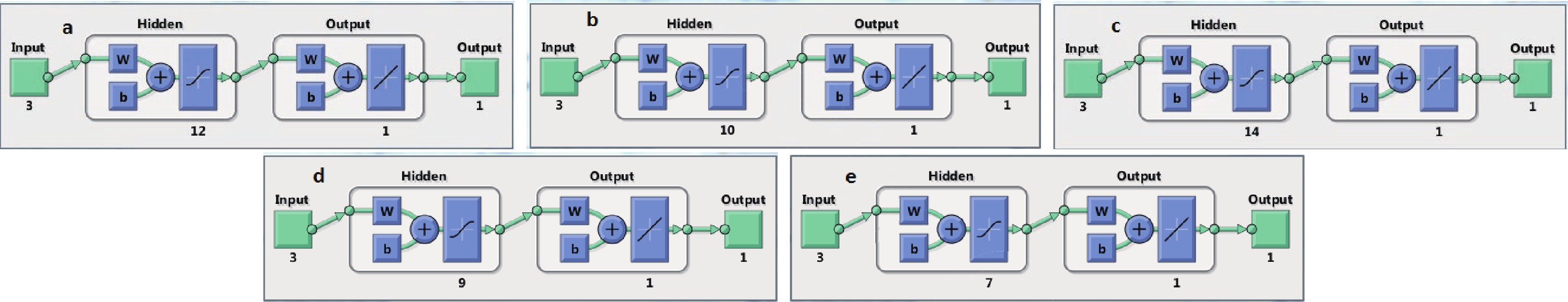
Figure 9. (color online) Same as in Fig. 4 but for particles (a) π, (b) k, (c) p, (d) Λ, and (e)
$ K_s^0 $ at$ \sqrt{s} = 5.02 $ TeV.As a result, the obtained best performance and regression values from the training, test, and validation sets are shown in Figs. 10 and 11 for particles (a) π, (b) k, (c) p, (d) Λ, and (e)
$ K_s^0 $ . This performance is obtained after epochs$ 19 $ ,$ 47 $ ,$ 8 $ ,$ 9 $ , and$ 14 $ for particles (a) π, (b) k, (c) p, (d) Λ, and (e)$ K_s^0 $ and is presented in Table 5. The transfer function used is tansig in the hidden layer for all particles and purelin in the output layer for all particles. All the parameters used for the ANN are shown in Table 5.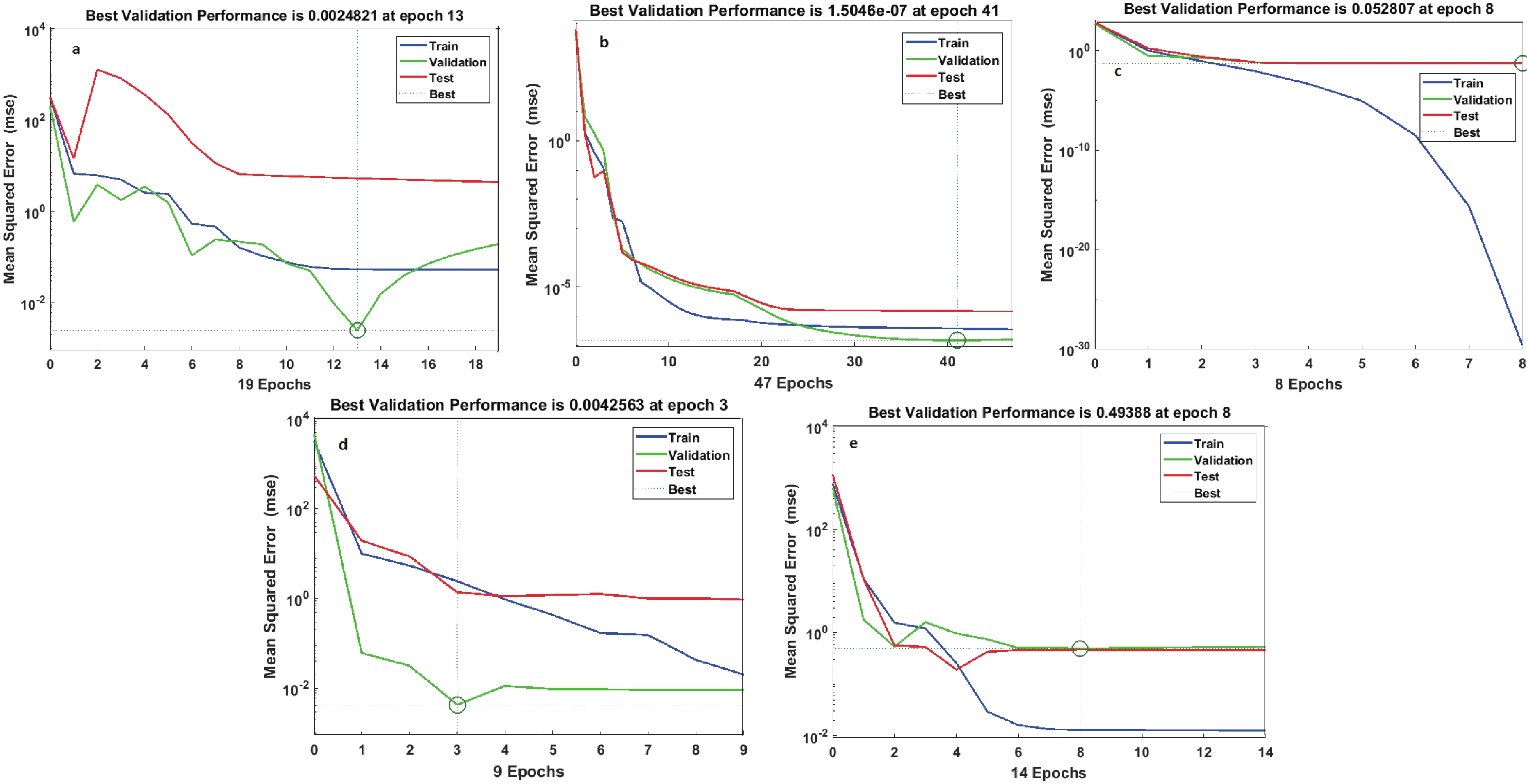
Figure 10. (color online) Same as in Fig. 5 but for particles (a) π, (b) k, (c) p, (d) Λ, and (e)
$ K_s^0 $ at$ \sqrt{s} = 5.02 $ TeV.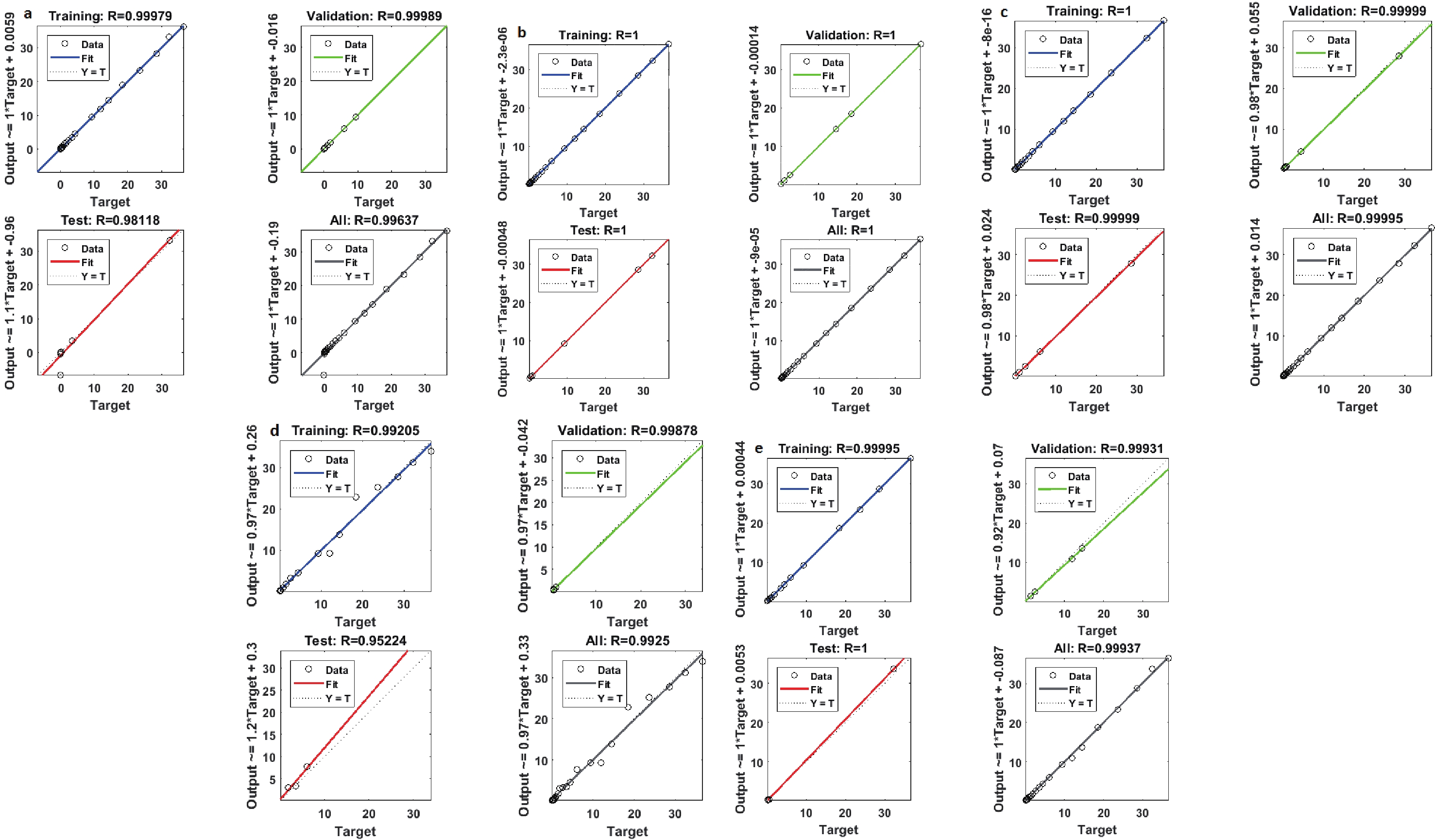
Figure 11. (color online) Same as in Fig. 6 but for particles (a) π, (b) k, (c) p, (d) Λ, and (e)
$ K_s^0 $ at$ \sqrt{s} = 5.02 $ TeV.Extrapolation of the observed transverse momentum spectra to
$ p_{\rm T} = 0 $ is necessary to determine the entropy S. To achieve this, we fit both the experimental and simulated$p_{\rm T}$ spectra to two various functional models, the Tsallis distribution [11, 12] and HRG model [13]. The aim of combining two models is to fit the entire$ p_{\rm T} $ curve.In Fig. 12, the experimental and simulated particle spectra
$ p_{\rm T} $ are compared to the Tsallis distribution and the HRG model for particles π (a), k (b), p (c), Λ (d), Ω (e), and$ \bar{\Sigma} $ (f). As shown in Fig. 8, employing various forms of the fitting function is suitable because the Tsallis function can only match the left side of the$ p_T $ curve at$ 0.001 < y < 10 $ , whereas the HRG model can fit the right side at$ 10 < y < 20 $ . This result may motivate us to pursue additional research. Tables 6 and 7 summarize the fitting parameters obtained from the Tsallis distribution and HRG model, respectively.Particle Tsallis parameters HRG model $ \chi^{2} $ /dof

$ {\rm d}N/{\rm d}y $ 

T/GeV q V/ $ {\rm fm}^3 $ 

T/GeV μ/GeV π $ 5804.25 $ 

$ 0.2101 $ 

$ 1.1218 $ 

$ 4709.14 \pm 1351.88 $ 

$ 2.6497 \pm 0.0475 $ 

$ 26.2268 \pm 0.7773 $ 

$ 316/48 $ 

K $ 953.214 $ 

$ 0.2392 $ 

$ 1.1146 $ 

$ 3614.78 \pm 1.6854 $ 

$ 0.719156 \pm 630181 $ 

$ 1.28019 \pm 630181 $ 

$ 905.7/44 $ 

p $ 437.394 $ 

$ 0.3393 $ 

$ 1.1167 $ 

$ 8.6667 \pm 3.7659 $ 

$ 3.45715 \pm 0.1372 $ 

$ 22.842 \pm 1.8419 $ 

$ 219.6/36 $ 

Λ $ 466.969 $ 

$ 0.4920 $ 

$ 1.119 $ 

$ 395.622 \pm 44731.7 $ 

$ 1.49141 \pm 15.7463 $ 

$ 10.0101 \pm 226.948 $ 

$ 198/16 $ 

$ K_s^0 $ 

$ 750.684 $ 

$ 0.4003 $ 

$ 1.105 $ 

$ 72.7633 \pm 82.7046 $ 

$ 2.5859 \pm 0.227 $ 

$ 17.809 \pm 3.2296 $ 

$ 547.7/18 $ 

Particle Tsallis fitting parameters HRG model fitting parameters $ \chi^{2} $ /dof

${\rm d}N/{\rm d}y $ 

$ T_{Ts} $ /GeV

q V/ $ {\rm fm}^3 $ 

$ T_{\tm th} $ /GeV

μ/GeV π $ 5807.58 $ 

$ 0.2099 $ 

$ 1.1221 $ 

$ 4681.65 \pm 1995.89 $ 

$ 2.5486 \pm 0.066 $ 

$ 24.7643 \pm 1.0789 $ 

$ 3173/48 $ 

K $ 958.826 $ 

$ 0.2396 $ 

$ 1.1159 $ 

$ 5871.87 \pm 4273.75 $ 

$ 3.202 \pm 0.1495 $ 

$ 36.6246 \pm 2.627 $ 

$ 9116.2/44 $ 

p $ 440.362 $ 

$ 0.3341 $ 

$ 1.1223 $ 

$ 1981.5 \pm 1398.83 $ 

$ 4.5297 \pm 0.2092 $ 

$ 59.7687 \pm 3.7575 $ 

$ 2246.4/36 $ 

Λ $ 472.765 $ 

$ 0.4976 $ 

$ 1.1183 $ 

$ 396.77 \pm 53486.2 $ 

$ 1.42152 \pm 15.2713 $ 

$ 9.10505 \pm 220.834 $ 

$ 1949.7/16 $ 

$ K_s^0 $ 

$ 749.794 $ 

$ 0.3945 $ 

$ 1.108 $ 

$ 26.688 \pm 55.3559 $ 

$ 2.0758 \pm 0.4493 $ 

$ 9.7132 \pm 5.5569 $ 

$ 5558.9/18 $ 

Table 7. Same as in Table 7, but the statistical fit results, from both used models, are compared to those of the ANN simulation model.

Figure 12. (color online) Transverse momentum distribution measured by the ALICE experiment collaboration [41, 42] at a centre of mass energy
$ = 5.02 $ TeV, which is represented by blue open circles for particles π (a), k (b), p (c), Λ (d), and$ K_s^0 $ (e), is compared to the statistical fits from the Tsallis distribution, which has perfect fits at$ 0.001 < y < 10 $ and is represented by red solid lines, given by Eq. (40), and the HRG model, which works in$ 10 < y < 20 $ and is represented by green solid lines, given by Eq. (35). A border line is drawn between the Tsallis and HRG models, shown in purple. The experimental data and the results of both models are then compared to that obtained from the ANN simulation model, represented by dark brown plus signs. The prediction of the ANN model is presented by red closed circles.The estimated entropy per rapidity
$ {\rm d}S/{\rm d}y $ from Pb-Pb central collisions at$ \sqrt{s} = 5.02 $ TeV using the Tsallis distribution, HRG model, and ANN model for particles π, k, p, Λ, and$ K_s^0 $ is represented in Table 8. The effect of both the Tsallis distribution and HRG model fitting functions on the estimated entropy per rapidity$ {\rm d}S/{\rm d}y $ is also shown in Table 8.Particle $ ({\rm{d}} S/{\rm{d}}y)_{y=0} $ 

$ ({\rm{d }}S/{\rm{d}}y)_{y=0} $ supplemented by Tsallis

$ (d S/dy)_{y=0} $ supplemented by HRG model

$ ({\rm{d }}S/{\rm{d}}y)_{y=0} $ estimated by ANN model

π $ 13188.2 $ 

$ 13406.9 $ 

$ 13333.6 $ 

$ 13330.9 $ 

K $ 3909.58 $ 

$ 3938.4 $ 

$ 1011.8 $ 

$ 3896.25 $ 

p $ 2259.36 $ 

$ 2262.64 $ 

$ 2250.08 $ 

$ 2253.3 $ 

Λ $ 2104.91 $ 

$ 2193.98 $ 

$ 2179.42 $ 

$ 2178 $ 

$ K_s^0 $ 

$ 2463.9 $ 

$ 3396.13 $ 

$ 3372.08 $ 

$ 3369.06 $ 

Table 8. Same as in Table 4 but at
$ \sqrt{s} =5.02 $ TeV.The values of the entropy per rapidity
$ {\rm{d }}S/{\rm{d }}y $ calculated by fitting the experimental and simulated particle spectra to the statistical models are in agreement. Better knowledge of the full created entropy in high energy heavy ion collisions is important for determining the bulk properties of both initial and final state quantities. The function that describes the non-linear relationship between the inputs and output is given in Appendix D. -
In this study, we calculate the entropy per rapidity
$ {\rm{d }}S/{\rm{d }}y $ produced in central Pb-Pb ultra-relativistic nuclear collisions at LHC energies using experimentally observed identifiable particle spectra and source radii estimated from HBT correlations. The considered particles are π, k, p, Λ, Ω, and$ \bar{\Sigma} $ and π, k, p, Λ, and$ K_s^0 $ with center of mass energies of$ \sqrt{s} =2.76 $ and$ 5.02 $ TeV, respectively. The ANN simulation model is used to estimate the entropy per rapidity$ {\rm{d }}S/{\rm{d }}y $ for the same particles at the considered energies. Extrapolating the transverse momentum spectra at$ p_{\rm T} =0 $ is required to calculate$ {\rm{d }}S/{\rm{d }}y $ ; thus, we use two different fitting functions, the Tsallis distribution and HRG model. The effect of both the Tsallis distribution and HRG model fitting functions on the estimated entropy per rapidity$ {\rm{d }}S/{\rm{d }}y $ is also discussed. The Tsallis function can only match the left side of the$ p_{\rm T} $ curve, whereas the HRG model can fit the right side. This result may motivate us to pursue additional research. The success of the ANN model in describing the experimental measurements implies further prediction for the entropy per rapidity in the absence of experiments. -
According to the Gibbs-Duhem relation, thermodynamic quantities are related by [43]
$ E(V, T, {\boldsymbol{\mu}})={\boldsymbol{F}}^{\prime}(V, T, {\boldsymbol{\mu}})+T S(V, T, {\boldsymbol{\mu}})+{\boldsymbol{\mu}} {\boldsymbol{b}}(V, T, {\boldsymbol{\mu}}) \tag{A1}. $

Thus, the entropy
$ (S) $ can be obtained as [43]$ S=\frac{1}{T}\left(E-{\boldsymbol{F}}^{\prime}-{\boldsymbol{\mu}} {\boldsymbol{b}}\right)=\ln Z-\beta \frac{\partial \ln Z}{\partial \beta}-(\ln \lambda) {\boldsymbol{\lambda}} \frac{\partial \ln Z}{\partial \lambda}\tag{A2}.$

Our aim is to express
$ (S) $ in terms of$ (f) $ , which is the single particle distribution function and is given by [43]$ \mathrm{f}_{F / \beta}(\xi, {\boldsymbol{\beta}}, \lambda)=\frac{1}{{\rm e}^{\,\beta(\xi-\mu)} \pm \mathbf{1}} \tag{A3},$

where
$ (+) $ and$ (-) $ represent fermions and bosons, respectively.The partition function (
${\rm ln} \,Z$ ) is given by [43]$ \ln Z_{F / \beta}({\boldsymbol{V}}, {\boldsymbol{\beta}}, \lambda)=\pm \int \frac{{\rm d}^{3} r {\rm d}^{3} P}{(2 \pi)^{3}} \ln \left[1 \pm {\bf{e}}^{\,\beta(\mu-\xi)}\right].\tag{A4} $

Differentiating Eq. (16) with respect to β, the inverse of temperature, we get [43]
$ \begin{aligned}[b] \frac{\partial \ln Z_{F / \beta}}{\partial \beta}=&\pm \int \frac{{\rm d}^{3} r {\rm d}^{3} P}{(2 \pi)^{3}} \frac{({\boldsymbol{\mu}}-{\boldsymbol{\xi}}) {\bf{e}}^{{\,\boldsymbol{\beta}}(\mu-\xi)}}{1 \pm {\bf{e}}^{{\,\boldsymbol{\beta}}(\mu-\xi)}}\\ =&\pm \int \frac{{\rm d}^{3} r {\rm d}^{3} P}{(2 \pi)^{3}} \frac{(\mu-\xi)}{{\rm e}^{\beta(\xi-\mu)} \pm 1}. \end{aligned} \tag{A5}$

Furthermore, differentiating Eq. (16) with respect to λ, we obtain [43]
$ \frac{\partial \ln Z}{\partial \lambda}=\pm \int \frac{{\rm d}^{3} r {\rm d}^{3} P}{(2 \pi)^{3}} \frac{{\bf{e}}^{{\,\boldsymbol{\beta}}(\mu-\xi)}}{1 \pm {\bf{e}}^{{\,\boldsymbol{\beta}}({\boldsymbol{\mu}}-\xi)}}. \tag{A6} $

Eq. (18) can be arranged as [43]
$\frac{\partial \ln Z}{\partial \lambda}=\pm \int \frac{{\rm{d}}^{3} r {\rm{d}}^{3} P}{(2 \pi)^{3}} \frac{1}{{\rm e}^{\,\beta(\xi-\mu)} \pm 1}. \tag{A7}$

Substituting Eqs. (16), (17), and (19) into Eq. (14), we get [43]
$ \begin{aligned}[b]S=&\pm \int \frac{{\rm d}^{3} r {\rm d}^{3} P}{(2 \pi)^{3}}\left[\ln \left(1 \pm {\rm e}^{\,\beta(\mu-\xi)}\right)-\frac{\beta(\mu-\xi)}{{\rm e}^{\,\beta(\mu-\xi)} \pm 1}\right. \\& \left.-\frac{\beta \mu {\rm e}^{\,\beta \mu}}{{\rm e}^{\,\beta(\xi-\mu)} \pm \mathbf{1}}\right] \end{aligned}\tag{A8} $

At vanishing chemical potential,
$ \mu_B=0 $ , the last term in Eq. (20) will equal zero.$ {\bf{e}}^{{\,\boldsymbol{\beta}}(\xi-{\boldsymbol{\mu}})} \pm \mathbf{1}=\frac{1}{{f}_{F / \beta}}. \tag{A9} $

Eq. (15) can be written in the following form [43]
$ -{\rm e}^{\beta(\xi-\mu)}=\frac{1}{{f}_{F / \beta}} \mp 1=\frac{1 \pm {f}_{F / \beta}}{{f}_{F / \beta}}, \tag{A10}$

and recalling Eq. (22), we obtain
$ -{\rm e}^{{\,\boldsymbol{\beta}}({\boldsymbol{\mu}}-\xi)}=\frac{{f}_{F / \beta}}{1 \mp {f}_{F / \beta}}. \tag{A11} $

Rearranging Eq. (23) in the following form:
$ \begin{aligned}[b] 1 \pm {\rm e}^{\,\beta(\mu-\xi)}=&1 \pm \frac{{f}_{F / \beta}}{1 \mp {f}_{F / \beta}}=\frac{1 \mp {f}_{F / \beta} \pm {f}_{F / \beta}}{1 \mp {f}_{F / \beta}}\\&-\frac{1}{1 \mp {f}_{F / \beta}}=1 \pm {\rm e}^{\,\beta(\mu-\xi)}. \end{aligned} \tag{A12}$

Substituting Eq. (24) into Eq. (20), we get
$ S=\pm \int \frac{{\rm d}^{3} r {\rm d}^{3} P}{(2 \pi)^{3}}\left[\ln \left(\frac{1}{1 \mp {f}_{F / \beta}}\right)-\ln \left(\frac{{f}_{F / \beta}}{1 \mp {f}_{F / \beta}}\right) {f}_{F / \beta}-z e r o\right]. \tag{A13}$

We rearrange Eq. (25) as
$ \begin{aligned}[b] S=&\pm \int \frac{{\rm{d}}^{3} r {\rm{d}}^{3} P}{(2 \pi)^{3}}\Big[-\ln \left(1 \mp {f}_{F / \beta}\right)\\&-\left[\ln {f}_{F / \beta}-\ln \left(1 \mp {f}_{F / \beta}\right)\right] {f}_{F / \beta}\Big]. \end{aligned}\tag{A14} $

Then, simplify Eq. (26) to
$ \begin{aligned}[b] S=&\pm \int \frac{{\rm{d}}^{3} r {\rm{d}}^{3} P}{(2 \pi)^{3}}\left[-\ln \left(1 \mp {f}_{F / \beta}\right)-{f}_{F / \beta} \ln {f}_{F / \beta}\right. \\ &\left.+{f}_{F / \beta} \ln \left(1 \mp {f}_{F / \beta}\right)\right]. \end{aligned}\tag{A15} $

Finally, the entropy S can be given by [43]
$ \begin{aligned}[b] S=&\pm \int \frac{{\rm{d}}^{3} r {\rm{d}}^{3} P}{(2 \pi)^{3}}\left[-{f}_{F / \beta} \ln \left(1 \mp {f}_{F / \beta}\right)-{f}_{F / \beta} \ln {f}_{F / \beta}\right. \\& \left.+{f}_{F / \beta} \ln \left(1 \mp {f}_{F / \beta}\right)\right]. \end{aligned} \tag{A16} $

Eq. (28) represents the entropy equation shown in Eq. (1).
-
The partition function
$ Z(T,V,\mu) $ is given by$ Z(T,V,\mu)=\rm{Tr}\left[\exp\left(\frac{{\mu}N-H}{\mathtt{T}}\right)\right], \tag{B1} $

where H represents the system's Hamiltonian, μ is the chemical potential, and N is the net number of all constituents. In the HRG approach, Eq. (29) can be written as a summation of all hadron resonances.
$ \begin{aligned}[b] \ln Z(T,V,\mu)=&\sum_i{{\ln Z}_i(T,V,\mu)} =\frac{V g_i}{(2{\pi})^3}\\ &\times \int^{\infty}_0{\pm {\rm d}^{3}p {\ln} {\left[1\pm \exp\left(\frac{E-\mu_{i}}{\mathtt{T}} \right) \right]}}, \end{aligned}\tag{B2} $

where
$ \pm $ represent bosons and fermions, respectively, and$ E_{i}=\left(p^{2}+m_{i}^{2}\right)^{1/2} $ is the energy of the i-th hadron.The particle's multiplicity can be determined from the partition function as
$ N_{i}=T \frac{\partial Z_{i}(T, V)}{\partial \mu_{i}}=\frac{V g_i} {(2{\pi})^3}\int^{\infty}_0{{\rm d}^{3}p \left[\exp\left(\frac{E-\mu_{i}} {\mathtt{T}}\right)\pm1\right]^{-1}}. \tag{B3} $

For a partially radiated thermal source, the invariant momentum spectrum is obtained as [43]
$ E\frac{{\rm d}^{3}N_{i}}{{\rm d}^{3}p}=E \frac{V g_i} {(2{\pi})^3}\left[\exp\left(\frac{E-\mu_{i}} {T}\right)\pm1\right]^{-1}. \tag{B4} $

The i-th particle's energy
$ E_{i} $ can be written as a function of the rapidity$ \left(y\right) $ and$ m_{\rm T} $ as$ E=m_{\rm T} \cosh\left(y\right). \tag{B5} $

Here,
$ m_{\rm T} $ represents the transverse mass and can be expressed in terms of the transverse momentum$ p_{\rm T} $ by$ m_{\rm T}=\sqrt{m^{2}+p_{\rm T}^{2}}. \tag{B6} $

Substituting Eq. (33) into Eq.(32), we obtain the particle momentum distribution at mid-rapidity (
$ y= 0 $ ) and$ \mu \neq 0 $ $ \frac{1}{2 \pi p_{\rm T}} \frac{{\rm d}^2N}{{\rm d}y{\rm d}p_{\rm T}}= \frac{V g_i m_{\rm T}} {(2{\pi})^3}\left[\exp\left(\frac{m_{\rm T}-\mu_{i}} {T}\right)\pm1\right]^{-1}. \tag{B7}$

We fit the experimental data of the particle momentum spectra with that calculated using Eq. (35), where the fitting parameters are V, μ, and
$T $ . -
The transverse momentum distribution of the produced hadrons at LHC energies is expressed as [11, 12]
$ \left.\frac{1}{p_{\rm T}} \frac{{\rm d}^{2} N}{{\rm d} p_{T} {\rm d} y}\right|_{y=0}=g V \frac{m_{\rm T}}{(2 \pi)^{2}}\left[1+(q-1) \frac{m_{\rm T}}{T}\right]^{-q /(q-1)}, \tag{C1} $

where
$ m_{\rm T} $ and$ p_{\rm T} $ represent the transverse mass and transverse momentum, respectively, y is the rapidity, g is the degeneracy factor, and V is the volume of the system.The obtained values of q and T represent a system in the kinetic freeze-out case.
In the limit where
$ q->1 $ , Eq. (36) is a simplification of the conventional Boltzmann distribution [11, 12].$ \left.\lim _{q \rightarrow 1} \frac{1}{p_{\rm T}} \frac{{\rm d}^{2} N}{{\rm d} p_{\rm T} {\rm d} y}\right|_{y=0}=g V \frac{m_{\rm T}}{(2 \pi)^{2}} \exp \left(-\frac{m_{\rm T}}{T}\right). \tag{C2} $

As a result, several statistical mechanics ideas may be applied to the distribution provided in Eq. (36).
Integrating Eq. (36) though the transverse momentum, we obtain [11, 12]
$ \begin{aligned}[b] \left.\frac{{\rm d} N}{{\rm d} y}\right|_{y=0} =&\frac{g V}{(2 \pi)^{2}} \int_{0}^{\infty} p_{\rm T} {\rm d} p_{\rm T} m_{\rm T}\left[1+(q-1) \frac{m_{\rm T}}{T}\right]^{-{q}/({q-1})} \\ =&\frac{g V T}{(2 \pi)^{2}}\left[\frac{(2-q) m_{0}^{2}+2 m_{0} T+2 T^{2}}{(2-q)(3-2 q)}\right] \\ &\times\left[1+(q-1) \frac{m_{0}}{T}\right]^{-{1}/({q-1})}, \end{aligned}\tag{C3} $

where
$ m_{0} $ is the mass of the used particle.From Eq. (38), the volume of the system can be written in terms of the multiplicity per rapidity
$ {\rm d}N /{\rm d}y $ and the Tsallis parameters q and T as$ \begin{aligned}[b] V=&\left.\frac{d N}{d y}\right|_{y=0} \frac{(2 \pi)^{2}}{g T}\left[\frac{(2-q)(3-2 q)}{(2-q) m_{0}^{2}+2 m_{0} T+2 T^{2}}\right]\\&\times\left[1+(q-1) \frac{m_{0}}{T}\right]^{{1}/({q-1})}. \end{aligned} \tag{C4}$

Substituting Eq. (39) into Eq. (38), we obtain the transverse momentum spectra.
$ \begin{aligned}[b] \left.\frac{1}{p_{\rm T}} \frac{{\rm d}^{2} N}{{\rm d} p_{\rm T} {\rm d} y}\right|_{y=0}=&\left.\frac{{\rm d} N}{{\rm d} y}\right|_{y=0} \frac{m_{\rm T}}{T} \frac{(2-q)(3-2 q)}{(2-q) m_{0}^{2}+2 m_{0} T+2 T^{2}}\\& \times\left[1 +(q - 1) \frac{m_{0}}{T}\right]^{{1}/({q-1})} \left[1 +(q - 1) \frac{m_{\rm T}}{T}\right]^{-{q}/({q-1})}. \end{aligned} \tag{C5}$

where
$ {\rm d} N/{\rm d} y $ ,$ T $ , and$q $ are the fitting parameters. -
The transverse momentum distribution
$ \dfrac{1}{N_{\rm evt} }\dfrac{{\rm d}^2 N}{ {\rm d} y {\rm d}p_{\rm T}} $ can be estimated from the ANN model as$ \begin{aligned}[b] \frac{1}{N_{\rm evt} }\frac{{\rm d}^2 N}{ {\rm d} y {\rm d} p_{\rm T}} =& {\rm purelin}[net.LW\left\{2,1\right\}{\rm tansig}(net.Iw\left\{1,1\right\}R\\&+net.b\left\{1\right\})+ net.b\left\{2\right\})]. \end{aligned}\tag{D1} $

Here, R represents the inputs (
$ \sqrt{S} $ ,$ p_{\rm T} $ , and centrality),$ IW $ and$ LW $ are the linked weights, represented as follows:$ net.IW \left\{1, 1\right\} $ is the linked weights between the input layer and hidden layer,$ net.LW \left\{2, 1\right\} $ is the linked weights between the hidden layer and output layer, and b is the bias, where$ net.b\left\{1\right\} $ is the bias of the hidden layer and$ net.b\left\{2\right\} $ is the bias of the output layer. -
Resilient propagation, or RPROP [44], is one of the fastest widely available training algorithms used for learning in multilayer feed forward neural networks for numerous applications with the extraordinary advantage of basic application. The RPROP algorithm simply alludes to the direction of the gradient. It is a supervised learning method. Resilient propagation calculates an individual delta
$ \Delta_{i j} $ for each connection, which determines the size of the weight update. The following learning rule is applied to calculate delta:$ \begin{equation} \begin{array}{c} \Delta_{i j}{ }^{(t)}=\left\{\begin{array}{l} \eta^+ \times \Delta_{i j}{ }^{(t-1)} ,\quad {\rm if}\quad \dfrac{\partial E}{\partial w_{i j}}^{(t-1)} \times \dfrac{\partial E^{(t)}}{\partial w_{i j}}>0 \\ \eta^- \times \Delta_{i j}{ }^{(t-1)}, \quad {\rm if} \quad \dfrac{\partial E}{\partial w_{i j}}^{(t-1)} \times \dfrac{\partial E^{(t)}}{\partial w_{i j}}<0 \\ \Delta_{i j}{ }^{(t-1)}, \rm { else } \end{array}\right. \end{array} \end{equation}\tag{E1} $

where
$ 0<\eta^-<1<\eta^+ $ .The update-amount
$ \Delta_{i j} $ developed during the learning process depends on the sign of the error gradient of the past iteration,${\partial E}/{\partial w_{i j}}^{(t-1)} $ and the error gradient of the present iteration,$ {\partial E}/{\partial w_{i j}}^{(t)} $ . Each time the partial derivative (error gradient) of the corresponding weight$ w_{i j} $ changes sign, which indicates that the last update was too large and the calculation has jumped over a local minimum, the update-amount$ \Delta_{i j} $ decreases by the factor$ \eta^{-} $ , which is a constant usually with a value of$ 0.5 $ . If the derivative retains its sign, the update amount slightly increases by the factor$ \eta^{+} $ to accelerate convergence in shallow regions.$ \eta^{+} $ is a constant usually with a value of 1.2. If the derivative is$ 0 $ , we do not change the update-amount. The weight-update is determined when the update-amount is obtained for each weight.The following equation is utilized to compute the weight-update:
$ \begin{equation} \begin{array}{c} \Delta w_{i j}^{(t)}=\left\{\begin{array}{l} -\Delta_{i j}{ }^{(t)}, \quad {\rm if }\quad \dfrac{\partial E^{(t)}}{\partial w_{i j}}>0 \\ +\Delta_{i j}{ }^{(t)},\quad {\rm if } \quad\dfrac{\partial E^{(t)}}{\partial w_{i j}}<0 \\ 0, \quad\rm { else } \\ w_{i j}^{(t+1)} = w_{i j}{ }^{(t)}+\Delta w_{i j}{ }^{(t)} \end{array}\right. \end{array}. \end{equation}\tag{E2} $

If the present derivative is a positive amount, suggesting that the past amount was also a positive amount (increasing error), the weight decreases by the update amount. If the present derivative is a negative amount, indicating that the past amount was also a negative amount (decreasing error), the weight increases by the update amount.
Entropy per Rapidity in Pb-Pb Central Collisions using Thermal and Artificial Neural Network (ANN) Models at LHC Energies
- Received Date: 2022-03-19
- Available Online: 2022-07-15
Abstract: The entropy per rapidity


 DownLoad: