


 Abstract
 HTML
HTML Reference
 Related
 PDF
PDF


-
Neutron stars (NSs) are a class of very dense stars in astronomy, and a long-running problem behind them is the equation of state of dense matter (EOS). However, owing to the non-perturbation processing of the strong interaction, we cannot directly learn the nuclear many-body problem from QCD [1, 2]. To overcome this issue, two major types of methods have been derived: (i) Ab-initio microscopic approaches combining bare two-body and three-body interactions to reproduce nucleon scattering data and few-body bound-state properties. To name a few, the typical series include the quantum Monte Carlo method [3], (Dirac)-Brueckner-Hartree-Fock [3–6] and Chiral effective field theory (
$ \chi EFT $ ) approach [7–11]. (ii) Phenomenonological methods use a limited number of adjustable coupling parameters to fit the properties of finite nuclei and nuclear matter by constructing effective interactions, which can effectively describe the ground-state properties and can be further extended to study NS matter; the typical ones like the Skyrme-Hartree-Fock method and the Relativistic Mean Field theory (RMFT) [12–18]. Among these many-body theories, the nucleon-nucleon short-range correlation (SRC) and its consequence in single-particle momentum distribution are some of the most essential and challenging topics [19–21]. Different studies have theoretically shown that this correlation effect originates from the strong repulsive core of nuclear force and its tensor part. Therefore, compared with the distribution of free Fermi gas, the nucleon momentum distribution caused by SRC can result in appreciable depletion below the Fermi surface, and some nucleons occupy above the Fermi surface, resulting in a high-momentum tail. Experiments have also confirmed the connection between the nucleon momentum distribution and the short-range correlation as$ (e, e'p) $ [22] and$ (e, e'NN) $ [23, 24]. Additionally, the proton-removal experiment using megaelectron-energy electron beams carried out in the Jefferson Lab laboratory showed that there is nearly 20% correlations in the$^{12}{\rm C}$ , and 90% of the correlations are in the form of p-n pairs [25].The SRC has vast implications in nuclear physics [26–31]; in Ref. [32], Y. Dewulf et al. presented an argument showing that the self-interacting SRC yield a saturation density closer to the empirical saturation density than the traditional Brueckner-Hartree-Fock method. Moreover, SRC also allows us to understand the EMC effect better [33, 34] and explain the density-dependent behavior of nuclear symmetry energy [29] and the neutrino-oscillation measurements [35, 36]. When it is extended to the study of NSs, the mass-radius relationship [37, 38], the tidal deformability [39], and the cooling will all be affected [40].
Any non-axisymmetric disturbances in NSs induced by dynamical instability such as rotating [41], magnetic reconfiguration, starquakes, and tidal forces in a close eccentric binary system [42, 43] will cause non-radial oscillations and radiate gravitational waves. In fact, through the latter, one can expect to decode important information about stellar parameters including mass-radius, magnetic field distribution, rotational rate, internal structure and EOS [44–48]. The nonradial oscillations in isolated NSs can be divided into polar (or even) oscillations that only produce spheroidal deformations in the fluid and axial (or odd) oscillations that produce toroidal deformations [49, 50], and the different oscillation patterns are characterized as fundamental
$ f $ -modes, gravity$ g $ -modes, pressure$ p $ -modes, pure time$ w $ -modes, and rotational$ r $ -modes according to different force [50–52]. As we know, the non-radial oscillations of NSs are also accompanied by radial oscillations [53]. Although radial oscillations cannot directly generate gravitational radiation, it can become coupled with it and amplify it [53, 54]. There has been numerous studies on radial and non-radial oscillations, for example, by studying the oscillations of NSs, we can determine the differences caused by internal components to identify whether it is a hadronic star, a hybrid star, or a strange quark star [49, 55–61]. Additionally, by identifying the quasiperiodic oscillations observed in giant flares induced by the torsional oscillation of the NS, the crust properties of the NS can be effectively constrained [62–65]. Numerical relativity simulations have shown that the hypermassive NS generated by the binary NS merger may undergo strong radial oscillations and emit gravitational waves with a few kilohertz frequencies [66, 67], and recently, the detectability of frequencies such as the modulation of short gamma-ray (SGRB) signal has been analyzed [68].It is still unclear whether the SRC will affect the oscillation of NSs and further affect the frequency of gravitational waves. To the best of our knowledge, apart from some works that have discussed the influence of the SRC effect on the mass-radius relationship and tidal deformability of NSs [37, 39, 69], there has been no work on its influence on the oscillation of the NS. In this study, we introduce the short-range correlation effect of nucleons into the NS and discuss its influence on the non-radial and radial oscillation mode. With the further improvement of the sensitivity of gravitational wave detectors in the future, it will be possible to detect signals of this frequency, which will further verify the SRC effect inside the NS.
The paper is organized as follows: In Section II, we introduce the SRC effect under the relativistic mean field model and present the modified EOS with SRC. In Section III, we illustrate the construction of a set of relativistic parameters with SRC to describe the NS that meets the multi-messenger astronomy constraints from NICER, GW170817 and the observation of massive NSs. Sections IV and V discuss the influence of SRC on the non-radial and radial oscillations of NS, respectively. The last section is a summary. Appendix A presents the complete derivation of the nucleon coupling parameters and nuclear saturated properties under the SRC effect.
-
In this article, we adopt the SRC-revised RMFT with the
$ \sigma\omega\rho\delta\phi $ model, in which on the basis of traditional RMFT [70, 71] including scalar-isoscalar meson$ \sigma $ , vector-isoscalar meson$ \omega $ , and vector-isovector meson$ \rho $ , we introduce the SRC-revised effect and further consider the scalar-isovector meson$ \delta $ and strangeness-hidden meson$ \phi $ that only couples to the hyperons. The energy density and pressure under the mean field approximation are given as$ \begin{aligned}[b] \varepsilon =& \sum\limits_{B = N, H}\langle\psi_{B}^+ {\rm i} \dot{\psi}_{B}\rangle+\sum\limits_{l}\langle\psi_{l}^+ {\rm i} \dot{\psi}_{l}\rangle+\frac{1}{2} m_{\sigma}^{2} \sigma_{0}^{2}-\frac{1}{2} m_{\omega}^{2} \omega_{0}^{2}\\ &-\frac{1}{2} m_{\rho}^{2} \rho_{0}^{2}+\frac{1}{2} m_{\delta}^{2}\delta_{0}^{2}-\frac{1}{2} m_{\phi}^{2} \phi_{0}^{2}-\Lambda_{\omega}\left(g_{\rho B} \rho_{0}\right)^{2}\left(g_{\omega B} \omega_{0}\right)^{2}\\ & +\frac{1}{3}g_{2} \sigma_{0}^{3}+\frac{1}{4} g_{3} \sigma_{0}^{4}, \end{aligned} $

(1) and
$ \begin{aligned}[b] p =& \frac{1}{3} \sum\limits_{B = N, H}\langle\psi_{B}^+(-{\rm i} \alpha \cdot \nabla) \psi_{B}\rangle+\frac{1}{3} \sum\limits_{l}\langle\psi_{l}^+(-{\rm i} \alpha \cdot\nabla) \psi_{l}\rangle \\ & -\frac{1}{2} m_{\sigma}^{2} \sigma_{0}^{2}+\frac{1}{2} m_{\omega}^{2} \omega_{0}^{2}+\frac{1}{2} m_{\rho}^{2} \rho_{0}^{2}+\Lambda_{\omega}\left(g_{\rho B} \rho_{0}\right)^{2}\left(g_{\omega B} \omega_{0}\right)^{2}\\& -\frac{1}{2} m_{\delta}^{2}\delta_{0}^{2}+\frac{1}{2} m_{\phi}^{2} \phi_{0}^{2}-\frac{1}{3} g_{2} \sigma_{0}^{3}-\frac{1}{4} g_{3} \sigma_{0}^{4}. \end{aligned} $

(2) Where
$ B $ includes the nucleonic degrees of freedom$ N(n, p) $ and hyperonic degrees of freedom$ H(\Lambda, \Xi, \Sigma) $ , and$ l $ is the lepton degrees of freedom$ l(e, \mu) $ . Both$\langle\psi^{+} {\rm i} \dot{\psi}\rangle_{B, l}$ and$\langle\psi^{+}(-{\rm i} \alpha \cdot \nabla) \psi\rangle_{B, l}$ are directly related to the single-nucleon momentum distribution, and thus to the SRC effect. For the case of asymmetric nuclear matter, recent theoretical and experimental works have shown that the shape of single-nucleon distribution near the Fermi surface is approximately expressed as$ \sim1/k^{4} $ [28–30]. Additionally, various microscopic methods exhibit an approximately linear relationship between isospin-asymmetry and single-nucleon distribution; hence, we can use the nuclear momentum distribution as follows:$ f(k)_{p} = \left\{ \begin{array}{*{20}{l}} C_{1}^{(p)}, & k \leq k_{F}^{(p)} \\ \dfrac{C_{2}^{(p)}(1-\beta)}{k^{4}}, & k_{F}^{(p)}<k \leq \lambda k_{F}^{(p)} \\ 0, & k>\lambda k_{F}^{(p)} \end{array}\right. $

(3) $ f(k)_{n} = \left\{ \begin{array}{*{20}{l}} C_{1}^{(n)}, & k \leq k_{F}^{(n)} \\ \dfrac{C_{2}^{(n)}(1+\beta)}{k^{4}} , & k_{F}^{(n)}<k \leq \lambda k_{F}^{(n)} \\ 0, & k>\lambda k_{F}^{(n)} \end{array}\right. $

(4) where
$ \beta $ is the isospin-asymmetry and$ \lambda $ denotes the high-momentum cutoff. The momentum distribution of the deuteron points out the momentum cutoff$ \lambda $ at$ 2.75\pm0.25 $ [29, 72]. Experiments show that short-range correlated nucleons account for about 20%~25% of all nucleons [25, 73–74]. In order to facilitate the introduction of SRC into the RMFT, we take the cutoff value in this work as$ \lambda\simeq 2.75 $ and the proportion of the high-momentum nuclei as 25%. With two conditions of the normalization and 25% of the high-momentum nucleons in symmetric nuclear matter, we can determine the values of$ C_{1}^{(p)} = 1- $ $ 0.25(1-\beta) $ ,$ C_{2}^{(p)} = 0.25k_{F}^{(p)4}/(3-3/\lambda) $ ,$ C_{1}^{(n)} = 1-0.25(1+\beta) $ , and$ C_{2}^{(n)} = 0.25k_{F}^{(n)4}/(3-3/\lambda) $ . We take$ \beta $ as 0 and 1, corresponding to the symmetry nuclear matter (SNM) and pure neutron matter (PNM), respectively, which is consistent with Ref. [69]. Therefore, the energy density (1) and pressure (2) are revised as$ \begin{aligned}[b] \varepsilon =& \sum\limits_{B = N, H} \frac{1}{\pi^{2}} \int_{0}^{k_{B}} {\rm{\; d}} k k^{2} \sqrt{k^{2}+m^{* 2}}+\sum\limits_{l} \frac{1}{\pi^{2}} \int_{0}^{k_{l}} {\rm{d}} k k^{2} \sqrt{k^{2}+m_{l}^{2}}+\sum\limits_{B} \frac{1}{3 \pi^{2}} k_{B}^{3}\left(g_{\omega B} \omega_{0}+g_{\rho B} I_{3 B} \rho_{0}+g_{\phi B} I_{3 B} \phi_{0}\right)+\frac{1}{2} m_{\sigma}^{2} \sigma_{0}^{2}\\ &-\frac{1}{2} m_{\omega}^{2} \omega_{0}^{2}-\frac{1}{2} m_{\rho}^{2} \rho_{0}^{2}+\frac{1}{2} m_{\delta}^{2}\delta_{0}^{2}-\frac{1}{2} m_{\phi}^{2} \phi_{0}^{2}-\Lambda_{\omega}\left(g_{\rho B} \rho_{0}\right)^{2}\left(g_{\omega B} \omega_{0}\right)^{2}+\frac{1}{3}g_{2} \sigma_{0}^{3}+\frac{1}{4} g_{3} \sigma_{0}^{4}\\ &-\frac{0.25(1-\beta)}{\pi^{2}} \int_{0}^{k_{F}^{(n)}} {\rm{d}} k k^{2}\left(g_{\omega n} \omega_{0}+g_{\rho n} I_{3 n} \rho_{0}+\sqrt{k^{2}+m^{* 2}}\right) -\frac{0.25(1+\beta)}{\pi^{2}} \int_{0}^{k_{F}^{(p)}} {\rm{d}} k k^{2}\left(g_{\omega p} \omega_{0}+g_{\rho p} I_{3 p} \rho_{0}+\sqrt{k^{2}+m^{* 2}}\right)\\ &+\frac{C_{2}^{(n)}(1-\beta)}{\pi^{2}} \int_{k_{F}^{(n)}}^{\lambda k_{F}^{(n)}} {\rm{d}} k k^{2} \frac{\left(g_{\omega n} \omega_{0}+g_{\rho n} I_{3 n} \rho_{0}+\sqrt{k^{2}+m^{* 2}}\right)}{k^{4}}+\frac{C_{2}^{(p)}(1+\beta)}{\pi^{2}} \int_{k_{F}^{(p)}}^{\lambda k_{F}^{(p)}} {\rm{d}} k k^{2} \frac{\left(g_{\omega p} \omega_{0}+g_{\rho p} I_{3 p} \rho_{0}+\sqrt{k^{2}+m^{* 2}}\right)}{k^{4}} \end{aligned}, $ 
(5) and
$ \begin{aligned}[b] p =& \frac{1}{3} \sum\limits_{B = N, H} \frac{1}{\pi^{2}} \int_{0}^{k_{B}} {\rm{\; d}} k \frac{k^{4}}{\sqrt{k^{2}+m^{* 2}}}+\frac{1}{3} \sum\limits_{l} \frac{1}{\pi^{2}} \int_{0}^{k_{l}} {\rm{d}} k \frac{k^{4}}{\sqrt{k^{2}+m_{l}^{2}}}-\frac{1}{2} m_{\sigma}^{2} \sigma_{0}^{2}+\frac{1}{2} m_{\omega}^{2} \omega_{0}^{2}+\frac{1}{2} m_{\rho}^{2} \rho_{0}^{2}+\Lambda_{\omega}\left(g_{\rho B} \rho_{0}\right)^{2}\left(g_{\omega B} \omega_{0}\right)^{2}\\ & -\frac{1}{2} m_{\delta}^{2}\delta_{0}^{2}+\frac{1}{2} m_{\phi}^{2} \phi_{0}^{2}-\frac{1}{3} g_{2} \sigma_{0}^{3}-\frac{1}{4} g_{3} \sigma_{0}^{4}-\frac{1}{3} \frac{0.25(1-\beta)}{\pi^{2}} \int_{0}^{k_{F}^{(n)}} {\rm{d}} k \frac{k^{4}}{\sqrt{k^{2}+m^{* 2}}}+\frac{C_{2}^{(n)}(1-\beta)}{3\pi^{2}} \int_{k_{F}^{(n)}}^{\lambda k_{F}^{(n)}} {\rm{d}} k \frac{k^{4}}{k^{4}\sqrt{k^{2}+m^{* 2}}}\\& -\frac{1}{3} \frac{0.25(1+\beta)}{\pi^{2}} \int_{0}^{k_{F}^{(p)}} {\rm{d}} k \frac{k^{4}}{\sqrt{k^{2}+m^{* 2}}}+\frac{C_{2}^{(p)}(1+\beta)}{3\pi^{2}} \int_{k_{F}^{(p)}}^{\lambda k_{F}^{(p)}} {\rm{d}} k \frac{k^{4}}{k^{4}\sqrt{k^{2}+m^{* 2}}}. \end{aligned}. $

(6) We follow the standard NS calculation scheme, in the NS crust region, where the density is approximately
$ 6.3 \times 10^{-12} {\rm{fm}}^{-3} \leqslant n \leqslant 2.46 \times 10^{-4}{\rm{fm}}^{-3} $ ; we use the Baym-Pethick-Sutherland (BPS) EOS [75]. For the inner crust region with a range of$ 2.46 \times 10^{-4} {\rm{fm}}^{-3} \leqslant n \leqslant n_{t} $ , we use the polytropic EOSs parametrized form given by$ P = a+b \varepsilon^{4 / 3} $ [69, 76, 77], where constants a and b are associated with the core-crust transition$ n_{t} $ ; here, we adopt the thermodynamic criterion [78, 79] and use the iterative method to select the transition density so that the pressure calculated by the relativistic mean field is greater than or equal to the pressure by the polytropic EOSs parametrized form.In this study, we consider the static spherically symmetric background spacetime described by
$ \begin{array}{l} {\rm d} s^{2} = -{\rm e}^{\nu(r)} {\rm d} t^{2}+ {\rm e}^{\lambda(r)} {\rm d} r^{2}+r^{2}\left({\rm d} \theta^{2}+\sin ^{2} \theta {\rm d} \phi^{2}\right). \end{array} $

(7) After solving Einstein's equation, we obtain the Tolman-Oppenheimer-Volkoff (TOV) equation [80]
$ \frac{{\rm{d}} p}{{\rm{d}} r} = -\frac{(p+\varepsilon)\left(M+4 \pi r^{3} p\right)}{r(r-2 M)}, $

(8) $ \begin{array}{l} {\rm{d}} M = 4 \pi r^{2} \varepsilon {\rm{d}} r, \end{array} $

(9) and the corresponding metric function
$ \begin{array}{l} {\rm e}^{\lambda(r)} = (1-2m / r)^{-1}, \end{array} $

(10) $ \nu(r) = 2\int_{r}^{\infty} {\rm d} r^{\prime} \frac{{\rm e}^{\lambda\left(r^{\prime}\right)}}{r^{\prime 2}}\left(m+4 \pi r^{\prime 3} p\right). $

(11) Then, with the charge conservation and beta equilibrium condition, the mass and radius of NS can be solved.
-
There are already many parameter sets to describe finite nuclear matter and NSs such as the GM series [81], GL series [82], TM series [83], and NL series [84, 85]; however, none of them consider the SRC effect. To the best of our knowledge, some recent studies [37, 39, 69] introduced the SRC to discuss parameters in detail under the
$ \sigma\omega\rho $ -model and applied them to study NSs; however, the case of$ \sigma\omega\rho\delta\phi $ -model absorbing isovector-scalar meson$ \delta $ has not been released so far. In this work, with the SRC-revised RMFT, we will re-determine the values of the six nucleon coupling parameters, namely$ g_{\sigma N}, \; g_{\omega N}, \; g_{\rho N}, \; g_{\delta N}, \; b, \; c $ . These unknown parameters can be divided into two categories according to the isospin properties. One type includes the isospin-independent quantities (isoscalar) of$g_{\sigma N}, \; g_{\omega N}, $ $ b, \; c$ , whose values are determined through the binding energy per nucleon$ B/A $ , the incompressibility coefficient$ K $ , the nucleon effective mass$ m^{*} $ , and the saturation density$ n_{0} $ . The other type includes the isospin-dependent quantities (isovector) like$ g_{\rho N}, \; g_{\delta N} $ that are determined by the symmetry energy$E_{\rm sym}$ and its slope$ L $ . Their detailed arithmetic formulae are presented in Appendix A.In this study, we focus on the SRC effect; therefore, for simplification, we only selected isospin-independent
$ K $ and isospin-dependent$ L $ for comparison and changed their values within the range allowed by recent experiments and theories. For other saturation quantities, we select relatively credible values and keep them unchanged. Specifically, we adopt$n_{0} = 0.16\ \rm fm^{-3}$ [86, 87],$ m^{*} = 0.7 $ and$ B/A = -16$ MeV [86, 88]; moreover, the symmetry energy is chosen as$E_{\rm sym} = 32.5$ MeV within the accepted values based on recent experiments and theoretical calculations [1, 89–91]. For$ K $ , we follow the suggestions given in Refs. [1] and select$ K $ with an uncertain region within$200 \leq K\leq 280\;{\rm{MeV}}$ . In fact, determining the symmetric energy slope$ L $ is quite tricky, and usually the numerical range extracted using purely theoretical methods is roughly between$[30.6,\ 86.8]\;{\rm{ MeV}}$ [1, 89, 92–96]. Recently, a more accurate model-independent experiment, PREX-2, reported a very thick$ ^{208} $ Pb neutron skin thickness [97]. Based on this result and considering the strong correlation between the$R_{\rm skin}^{208}$ and$ L $ , Ref. [98] deduces a symmetry energy slope$ L $ up to$ (106\pm37) $ MeV, which challenges our understanding of the neutron-rich matter near the nuclear saturation density. In this work, we only selected a relatively small interval from$50~\rm MeV$ to 70 MeV with an interval of 5 MeV. We can observe that there are seven unknown parameters that need to be determined in the expressions of the energy density (5) and pressure (6) under SRC, whereas the properties of the saturated nuclear matter are only six; therefore, we still need to determine one parameter in advance. In this work, we chose$ \Lambda_{\omega} $ as a fixed value and take its value as 0.01 based on the previous research [18, 99]. Then, according to the derivation in Appendix A, the SRC-revised values of$ g_{\sigma N}, \; g_{\omega N}, \; b, \; c $ as well as$ g_{\rho N} $ and$ g_{\delta N} $ could be determined, as listed in Table 1.Number $K/\rm MeV$ 

$L/\rm MeV$ 

$ g_{\sigma N} $ [no-src]

$ g_{\omega N} $ [no-src]

$ b $ [no-src]

$ c $ [no-src]

$ g_{\rho N} $ [no-src]

$ g_{\delta N} $ [no-src]

(No.1) 200 50 10.08 [9.49] 9.28 [10.35] 36.39 [23.45] −102.62 [−58.63] 15.55 [13.84] 2.63 [6.37] (No.2) 220 50 9.99 [9.42] 9.28 [10.35] 32.71 [20.83] −86.31 [−47.66] 15.56 [13.83] 2.64 [6.36] (No.3) 240 50 9.91 [9.36] 9.28 [10.35] 29.13 [18.27] −70.72 [−37.07] 15.57 [13.81] 2.66 [6.35] (No.4) 260 50 9.82 [9.29] 9.28 [10.35] 25.66 [15.77] −55.83 [−26.86] 15.58 [13.79] 2.68 [6.34] (No.5) 280 50 9.73 [9.22] 9.28 [10.35] 22.28 [13.32] −41.63 [−17.02] 15.59 [13.78] 2.70 [6.33] (No.3) 240 50 9.91 [9.36] 9.28 [10.35] 29.13 [18.27] −70.72 [−37.07] 15.57 [13.81] 2.66 [6.35] (No.6) 240 55 9.91 [9.36] 9.28 [10.35] 29.13 [18.27] −70.72 [−37.07] 16.63 [14.75] 4.19 [6.92] (No.7) 240 60 9.91 [9.36] 9.28 [10.35] 29.13 [18.27] −70.72 [−37.07] 17.58 [15.60] 5.22 [7.39] (No.8) 240 65 9.91 [9.36] 9.28 [10.35] 29.13 [18.27] −70.72 [−37.07] 18.46 [16.39] 6.01 [7.80] (No.9) 240 70 9.91 [9.36] 9.28 [10.35] 29.13 [18.27] −70.72 [−37.07] 19.28 [17.12] 6.68 [8.17] Table 1. Relativistic nucleon coupling parameter sets constructed by the bulk properties of saturation nuclear matter. We have adopted
$ m_{B}=938.9\;{\rm{MeV}}, m_{\sigma}=538.6\;{\rm{MeV}}, m_{\omega}=783\;{\rm{MeV}}, m_{\rho}=769\;{\rm{MeV}}, m_{\delta}=979.9\;{\rm{MeV}}, $ $B/A=-16\;{\rm{MeV}}, n_{0}=0.16\;{\rm{fm}}^{-3}, m^{*}=0.7, E_{sym}= $ $ 32.5\;{\rm{MeV}} $ and$ \Lambda_{\omega}=0.01 $ [18, 99]. Select$ K $ with an uncertain region within$200 \leq K\leq 280\;{\rm{MeV}}$ and choose the credible value of$ L $ from$ 50\;{\rm{MeV}} $ to$ 70\;{\rm{MeV}} $ with an interval of$ 5\;{\rm{MeV}} $ . According to the derivation in Appendix A, nine groups of SRC-modified nucleon coupling parameters are constructed. The square brackets are the corresponding values with no-SRC effects. -
For the meson-hyperon coupling parameters, recent studies [100–102] have shown that the
$SU$ (6) quark symmetry group should be broken in favor of the$SU$ (3) group, in which case, all vector meson-hyperon coupling parameters can be expressed as a function of the vector parameter$ \alpha_{v} $ . Moreover, the value of$ \alpha_{v} $ generally lies between 0 and 1, and the$SU$ (3) will recover to$SU$ (6) when taking$ \alpha_{v} = 1 $ (see Ref. [101] for a review). In this study, we take the typical value of$ \alpha_{v} $ as 0.25. Within the$SU$ (3) group, the vector meson-hyperon coupling parameters$ g_{\omega H} $ are given as:$ \frac{g_{ \omega\Lambda }}{g_{ \omega N}} = \frac{4+2 \alpha_{v}}{5+4 \alpha_{v}}, \; \frac{g_{ \omega \Sigma }}{g_{\omega N}} = \frac{8-2 \alpha_{v}}{5+4 \alpha_{v}}, \; \frac{g_{ \omega\Xi }}{g_{ \omega N}} = \frac{5-2 \alpha_{v}}{5+4 \alpha_{v}}. $

(12) For the vector meson-hyperon coupling parameters
$ g_{\rho H} $ , we obtain$ \frac{g_{\rho \Lambda }}{g_{ \rho N}} = 0, \; \frac{g_{ \rho\Sigma}}{g_{ \rho N}} = 2 \alpha_{v}, \; \frac{g_{ \rho\Xi}}{g_{ \rho N}} = 2 \alpha_{v}-1, $

(13) and the vector meson-hyperon coupling parameter
$ g_{\phi H} $ are$ \begin{aligned}[b] \dfrac{g_{ \phi\Lambda}}{g_{ \omega N}} =& \sqrt{2}\left(\frac{2 \alpha_{v}-5}{5+4 \alpha}\right), \quad \dfrac{g_{ \phi\Sigma}}{g_{ \omega N}} = -\sqrt{2}\left(\frac{2 \alpha_{v}+1}{5+4 \alpha_{v}}\right)\\ \dfrac{g_{\phi\Xi }}{g_{ \omega N}} =& -\sqrt{2}\left(\frac{2 \alpha_{v}+4}{5+4 \alpha_{v}}\right), \end{aligned} $

(14) The next is the scalar meson-hyperon coupling parameter
$ g_{\delta H} $ :$ \frac{g_{\delta \Lambda }}{g_{ \delta N}} = 0, \; \frac{g_{ \delta\Sigma}}{g_{ \delta N}} = 2 \alpha_{v}, \; \frac{g_{ \delta \Xi}}{g_{ \delta N}} = 2 \alpha_{v}-1. $

(15) For the scalar meson-hyperon coupling parameters
$ g_{\sigma H} $ , it can be determined by fitting the hyperon potential with$ U_{H}^{N} = (g_{\omega H}/g_{\omega N}) V-(g_{\sigma H}/g_{\sigma N}) S $ , where$V = \left(g_{\omega N} / $ $ m_{\omega}\right)^{2} \rho_{0}$ and$ S = m-m^{*} $ denote the vector and scalar field strengths at the saturation density,$ U_{H}^{N} $ is the hyperon potential depth. In this work, we take the widely accepted values with$U_{\Lambda}^{N} = -28~ {\rm{MeV}}, \; U_{\Sigma}^{N} = +30~ {\rm{MeV}}, \; U_{\Xi}^{N} = $ $ -18~ {\rm{MeV}}$ [81, 103−106].Next, to examine the parameter sets constructed by
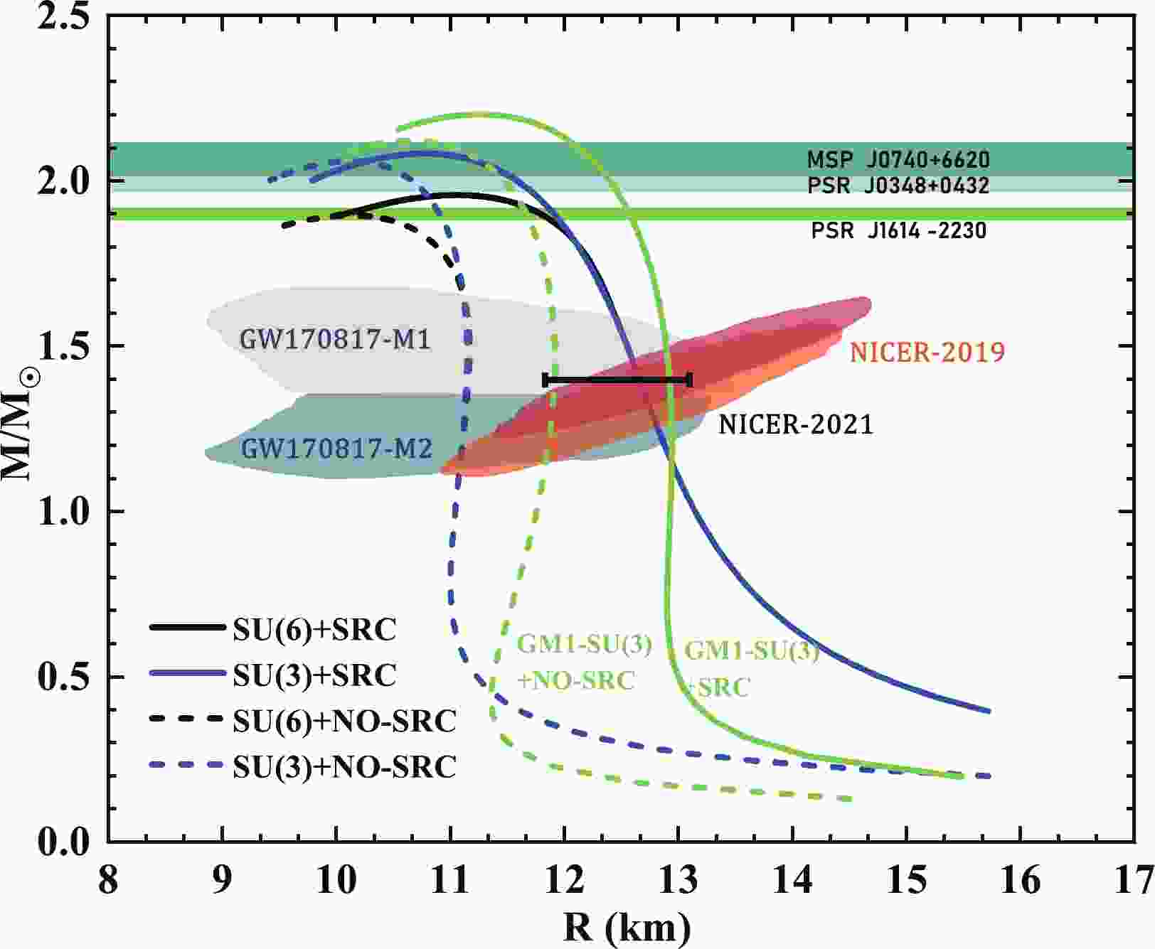
$SU$ (3) in the case of SRC, we selected (No.3) as a representative set and depicted the NS's mass-radius relationships in Fig. 1. The solid lines in the figure indicate the considered SRC effect. We found that the mass-radius relationship obtained by$SU$ (3) (blue solid lines) not only meet the three massive NSs given by recent astronomical observations [107-111], but also fall into the constraints given by the GW170817 gravitational wave event [112−116] and the state-of-the-art NICER [117−119], whereas the results by$SU$ (6), as shown by the black solid lines are difficult to meet the mass requirements. These indicate that when the NS contains hyperon components, the introduction of the SRC effect under the$SU$ (3) symmetry group can effectively avoid the hyperon puzzle (the existence of hyperons will soften EOSs and fail to meet the mass requirements), and also meet the astronomical constraints. For comparison with traditional RMF parameters, we have added an additional set of commonly used RMF parameters GM1 [81, 120] in Fig. 1, which effectively satisfy the observational constraints under$SU$ (3). It can be observed that the SRC has a similar effect on the GM1 parameter as it does on our constructed parameters, both causing an increase in the maximum mass and radius. This is because under the same RMF model, our constructed parameters and the GM1 set both depend on the properties of the saturated nuclear matter, and also have the same SRC-revised process. In the following discussion, we deduce that this conclusion is also applicable to other parameters in Table 1. For comparison, we have also drawn the results of no-SRC shown by the dotted lines.
Figure 1. (color online) The NS's mass-radius relationship calculated with or without SRC. The solid lines indicate that SRC is considered, whereas the dotted lines show that it is not. The green line represents a typical GM1 parameter set. The black and blue lines represent the
$SU$ (6) and$SU$ (3) group, respectively, and the shaded areas are the constraints from the GW170817 gravitational wave event and NICER-2019. The black horizontal line represents the latest restriction given by NICER-2021 (we use NICER-2019 and NICER-2021 to distinguish the NICER constraints from different years). The three light-colored square bars are the three massive NSs recently observed: PSR J1614-2230, PSR J0348+0432 and MSP J0740+ 6620.Presently, we have obtained the SRC-revised RMFT, and constructed nine SRC-revised coupling parameters within the range allowed by the nuclear saturation properties. Before discussing the impact of the SRC on the oscillation properties, we need to ensure that all the parameters constructed under this model can meet the current observations, including the maximum mass requirements, dimensionless tidal deformability, and NICER. Only by meeting these requirements can we further use it to discuss the oscillations.
a. Mass-NICER Constraints As mentioned above, we constructed nine groups of the parameters in Table 1, in which one type was constructed by isospin-independent
$ K $ and the other by isospin-dependent$ L $ . We use these two types to evaluate the influence of the SRC effect on the properties of NSs. In Fig. 1, we only show the mass-radius relationship with one set of parameters (No.3). To consider the SRC effect under different parameter sets, we plot the results in Fig. 2. It can be observed that SRC will increase the maximum mass and radius of NSs under both types of parameters. Particularly, for NS near$ 1.4M_{\odot} $ , compared to no-SRC, owing to the high-momentum nucleon occupation above the Fermi surface, the nucleons are relatively more difficult to be compressed [39, 69], resulting in a stiffer EOS and larger radius. When compared to the work [121], we deduce that the effect of the symmetry energy slope$ L $ is small. This may be due to the fact that the$ L $ are only taken from 50 MeV to 70 MeV (a range of 20 MeV), whereas the values given by the authors are taken from 20 MeV to 80 MeV (three times our span). Additionally, we consider the baryon octet; the appearance of hyperons also weakens the effect from$ L $ . For the mass$ > 2M_{\odot} $ , as the internal density increases, the nucleons gradually transform to hyperons, and the numbers of short-range associations decreases, but still leads to an increase in the maximum mass. We can observe that compared with the case of no-SRC, the introduction of SRC into RMFT will increase the radii of NSs and cause the results to better meet the multi-messenger observations, especially in the case of canonical NS restricted by NICER [117, 118]. It is worth noting that for the radius of the large-mass PSR J0740+6620, the latest analysis shows that its radius is roughly$ 12.35 \pm 0.75 $ [119]. Although the result we obtained is slightly smaller than this range, SRC is still closer to the constraint than no-SRC.
Figure 2. (color online) Under different parameters, the NS's mass-radius relationship calculated with or without SRC. The solid lines indicate that SRC is considered, whereas the dotted lines show that it is not. The black horizontal line represents the constraint from NICER-2021 and the three light-colored square bars are the three massive NSs of PSR J1614-2230, PSR J0348+0432 and MSP J0740+6620.
b. Tidal Deformability Constraints. With the help of LIGO and Virgo Collaboration [112, 113], the most significant phenomenon during the binary inspiral is that each NS will produce an observable dimensionless tidal deformability under the gravitational field of its companion star. It can be expressed in form of the second tidal Love number
$ k_{2} $ as$ \Lambda = 2k_{2}/(3C^{5}) $ with$ C $ being the compactness parameter ($ M/R $ ), where$ k_{2} $ can be calculated by the following expression [122–124]:$ \begin{aligned}[b] k_{2} =& \frac{8 C^{5}}{5}(1-2 C)^{2}\left[2+2 C\left({\mathcal{Y}}_{R}-1\right)-{\mathcal{Y}}_{R}\right]\\ & \times\bigg\{2 C\left[6-3 {\mathcal{Y}}_{R}+3 C\left(5 {\mathcal{Y}}_{R}-8\right)\right]\\& +4 C^{3}\left[13-11 {\mathcal{Y}}_{R}+C\left(3 {\mathcal{Y}}_{R}-2\right)+2 C^{2}\left(1+{\mathcal{Y}}_{R}\right)\right] \\& +3(1-2 C)^{2}\left[2-{\mathcal{Y}}_{R}+2 C\left({\mathcal{Y}}_{R}-1\right) \ln (1-2 C)\right]\bigg\}^{-1} \end{aligned}, $

(16) where
$ {\mathcal{Y}}_{R}\equiv{\mathcal{Y}}(R) $ is the solution of the first-order differential equation with the boundary condition$ {\mathcal{Y}}(0) = 2 $ ,$ r \frac{{\rm d} y(r)}{{\rm d} r}+y^{2}(r)+y(r) F(r)+r^{2} Q(r) = 0, $

(17) where
$ F(r) $ and$ Q(r) $ are expressed in the following form$ \begin{aligned}[b] F(r) =& \left[1-\frac{2 M(r)}{r}\right]^{-1}\left\{1-4 \pi r^{2}[{\mathcal{E}}(r)-P(r)]\right\} , \\ r^{2} Q(r) =& \left\{4 \pi r^{2}\left[5 {\mathcal{E}}(r)+9 P(r)+\frac{{\mathcal{E}}(r)+P(r)}{\dfrac{\partial P}{\partial {\mathcal{E}}}(r)}\right]-6\right\} \\ & \times\left[1-\frac{2 M(r)}{r}\right]^{-1}-\left[\frac{2 M(r)}{r}+2 \times 4 \pi r^{2} P(r)\right]^{2} \\& \times\left[1-\frac{2 M(r)}{r}\right]^{-2}. \end{aligned} $

(18) In Fig. 3 we show the relationship between the dimensionless tidal deformability and radius, where the solid line and dashed line indicate SRC and no-SRC respectively. First, the tidal deformability decreases with the mass in both cases, i.e. the larger the mass, the more difficult it is to produce tidal effects owing to its higher compactness parameter [114, 125]. The influence of the scalar parameters on the tidal deformability tends to be more obvious than that of vector ones. Additionally, two cases reach the same conclusion that the tidal deformability values given by SRC are both larger than those with no-SRC. This is because the dimensionless tidal deformability at a given mass strongly depends on the radius of the NS. According to recent research [114, 126–129], there is an empirical positive correlation function between
$ R_{1.4} $ and$ \Lambda_{1.4} $ ; we have observed that the radius with SRC at around$ 1.4 M_{\odot} $ is much larger than that with no-SRC in Fig. 2; therefore, a corresponding larger tidal deformability is expected. It is worth noting that our results show that the tidal deformability given by SRC is$ 200_{-10}^{+25} $ higher than no-SRC in the vicinity of$ 1.4M_{\odot} $ , and this is expected to provide a new perspective for the future observation of dimensionless tidal deformability. To determine whether the result meets the constraint from the GW170817 event with$ \Lambda_{1.4} = 190^{+390}_{-120} $ [113], we mark it with a vertical dark blue dotted line in the figure, and the results all fall into this interval. We also calculate the respective tidal deformability of two NSs in GW170817 event. Given the most credible value for the chirp mass with$ [(m_{1} m_{2})^{3 / 5}] /[(m_{1}+m_{2})^{1 / 5}] = 1.188 M_{\odot} $ [112], we plot the results in Fig. 4, in which$ \Lambda_{1} $ and$ \Lambda_{2} $ stand for the high-mass and low-mass, respectively. The dark blue dotted contour lines indicate the 90% and 50% credible interval, and our results are in line with these constraints. If the high-sensitivity detectors can detect more binary NS merger events in the future, the numerical range of tidal deformability will become increasingly accurate, and our results induced by SRC will be further tested.
Figure 3. (color online) NS radius-tidal deformability relationship calculated with and without SRC. The solid lines indicate that SRC is considered, whereas the dotted lines indicate that it is not. The vertical dotted line represents the tidal deformability range obtained from the analysis of the GW170817 event.

Figure 4. (color online) Relationship between
$ \Lambda_{1} $ and$ \Lambda_{2} $ in GW170817 gravitational event calculated with and without SRC. The solid lines indicate that SRC is considered, whereas the dotted lines indicate that it is not. The dark green contour lines represent the 90% and 50% credible intervals.So far, it can be observed that all the parameter sets constructed under the
$SU$ (3) group can meet the observation constraints. It should be noted that the introduction of the SRC effect, the structure of the NS, especially the radius, can be changed; there is still uncertainty in the choice of model parameters, especially the choice of the symmetry energy slope parameters. Different choices may lead to different interpretations, and these results are yet to be better understood before further precise determination of all the nuclear matter parameters. Next, we use the above parameters to determine the influence of SRC on NSs' oscillations. -
The discussion of non-radial modes under the framework of general relativity was originally proposed by Thorne and Campollataro [130]. For the non-rotating neutron star considered in our work, the interior is composed of an ideal fluid; we use the Cowling approximation approach [131–133], which ignores the space-time metric perturbation and only retains the density perturbations associated with the fluid oscillations inside the star [50]. Recent work shows that the difference between the f-mode calculated using the Cowling approximation approach and by the complete linearized equations of the general relativity is only less than 20%; the p-mode is approximately 10% [134], and the error of the g-mode is only a few percent [45]. This is enough to show the practicality of the Cowling approximation [135]. In this approximation the fluid perturbations are composed of a spherical harmonic function
$ Y_{l m}(\theta, \phi) $ and a time-dependent part${\rm e}^{{\rm i}\omega t}$ , and the Lagrangian fluid displacement associated with infinitesimal oscillatory perturbations is expressed as:$ \begin{aligned}[b] \zeta^{i} =& \left[{\rm e}^{-\Lambda(r)} W(r), -V(r) \partial_{\theta}, -V(r) \sin ^{-2} \theta \partial_{\phi}\right] r^{-2} \\ &\times Y_{l m}(\theta, \phi) {\rm e}^{{\rm i}\omega t}, \end{aligned} $

(19) where
$ W(r) $ and$ V(r) $ satisfy the following equations:$ \begin{aligned}[b] \frac{{\rm d} W(r)}{{\rm d} r} =& \frac{{\rm d} \varepsilon}{{\rm d} p}\left[\omega^{2} r^{2} {\rm e}^{\Lambda(r)-2 \phi(r)} V(r)+\frac{{\rm d} \Phi(r)}{{\rm d} r} W(r)\right]\\& -l(l+1) {\rm e}^{\Lambda(r)} V(r) , \end{aligned} $

(20) $ \frac{{\rm d} V(r)}{{\rm d} r} = 2 \frac{{\rm d} \Phi(r)}{{\rm d} r} V(r)-\frac{1}{r^{2}} {\rm e}^{\Lambda(r)} W(r) , $

(21) where
$ \frac{{\rm d} \Phi(r)}{{\rm d} r} = \frac{-1}{\varepsilon(r)+p(r)} \frac{{\rm d} p}{{\rm d} r}. $

(22) Given appropriate boundary conditions, the above equations are the eigenvalue equations of
$ \omega $ . In the NS interior ($ r = 0 $ ),$ W(r) $ and$ V(r) $ have the following approximate behaviors:$ \begin{array}{l} W(r) = A r^{l+1}, \quad V(r) = -\dfrac{A}{l} r^{l}, \end{array} $

(23) where A is an arbitrary constant. Another boundary condition is that in the NS surface area, the pressure will disappear:
$ \omega^{2} {\rm e}^{\Lambda(R)-2 \Phi(R)} V(R)+\left.\frac{1}{R^{2}} \frac{{\rm d} \Phi(r)}{{\rm d} r}\right|_{r = R} W(R) = 0. $

(24) In full general relativity (without the Cowling approximation), the solution of the perturbation equations is in complex form, with the real part corresponding to the mode frequency and the imaginary part corresponding to the damping time. However, in the Cowling approximation, the perturbation equations only give the real mode frequency
$ \omega $ . The numerical integrations of (20) and (21) with the initial conditions (23) are performed using the Runge-Kutta method, and the coefficients in the integrations are derived from the TOV equation (8) and (9). To solve the boundary conditions (24), we use the Newton-iterative algorithm, and given a suitable initial value we find the frequencies that satisfy the condition.Using the parameter set constructed above, we calculated the most typical non-radial
$ f $ -mode frequency for quadrupole oscillations ($ l $ = 2) [136] and showed the relationship between the$ f $ -mode and mass in Fig. 5. Two sets of parameters both show that the$ f $ -mode frequency increases with the mass, and the curve bends after reaching the maximum mass, which corresponds to an unstable NS. In the case of the isoscalar parameter$ K $ , a larger$ K $ leads to a smaller$ f $ -mode frequency, because a larger$ K $ means that the nuclear matter is more difficult to compress, which makes the NS more difficult to excite the oscillations. A different isoscalar parameter$ L $ has less effect on the$ f $ -mode.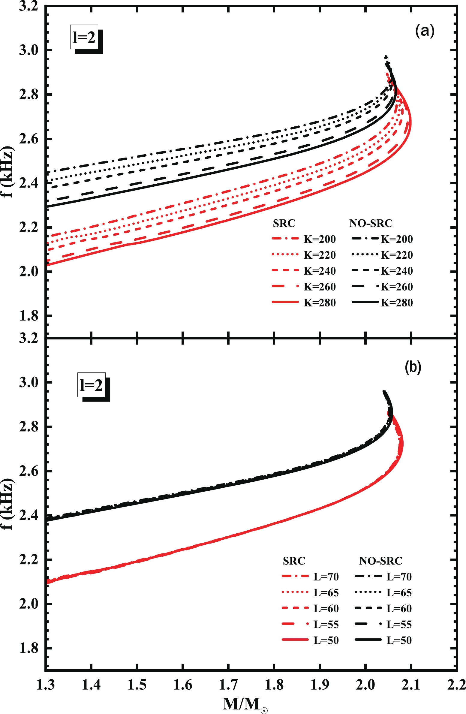
Figure 5. (color online) NS mass-
$ f $ mode frequency relationship calculated with and without SRC. We calculated the most typical non-radial$ f $ -mode frequency for quadrupole oscillations ($ l $ = 2). The black and red curves represent no-SRC and SRC, respectively.We can clearly observe that the SRC effect will significantly reduce the
$ f $ -mode frequency in all cases and this reduction is approximately$ 0.2\sim0.3 $ kHz. Specifically, after considering the SRC effect, for$ K $ , the corresponding$ f $ -mode frequency of$ 1.4M_{\odot} $ decreases from 2.32$ \sim $ 2.48 kHz to 2.08$ \sim $ 2.2 kHz, whereas that of$ 2M_{\odot} $ decreases from 2.64$ \sim $ 2.76 kHz to 2.44$ \sim $ 2.56 kHz. For$ L $ , the$ f $ -mode of$ 1.4M_{\odot} $ decreases from 2.42 kHz to 2.14 kHz and that of$ 2M_{\odot} $ decreases from 2.72 kHz to 2.52 kHz. It is easy to understand this result using the following discussion in Fig. 6. We know that the characteristic time scale of any dynamical process is related to the average density of the masses involved (see Misner, Thorne & Wheeler, 1973, chapter 36.4 formula (36.11a) and chapter 36.5 formula (36.15)); when applied to the stellar fluid oscillation modes, we expect that$ \omega_{f}\sim (\bar{M}/\bar{R}^{3})^{1/2} $ . This shows that the$ f $ -mode frequency has a strong dependence on the average density. As shown in Fig. 2, the introduction of the SRC will significantly increase the NS's radius, resulting in a decrease in the average density, thus a smaller average density corresponds to a smaller frequency.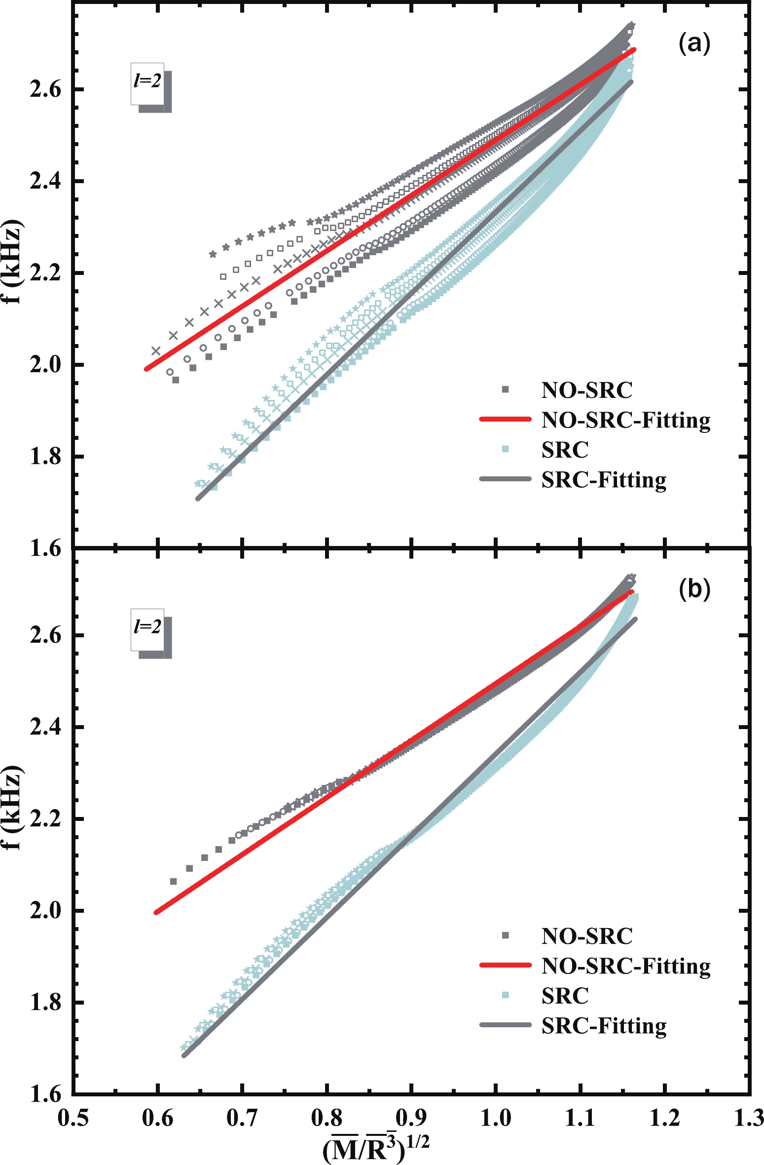
Figure 6. (color online) Linear relationships between
$ f $ -mode frequency and average density$ \sqrt{\frac{\bar{M}}{\bar{R}^{3}}} $ . The gray and light green points indicate no-SRC and SRC, respectively, whereas the solid line indicate the linear fitting result.GW asteroseismology allows us to relate the oscillation frequency of NS to its mass and radius and to obtain a universal relationship between them [136–141]. The original relation was proposed by Andersson and Kokkotas [44, 142]. Through the realistic EOS equation, they established the relationship between the average density and
$ f $ -mode frequency as$ \begin{array}{l} f({\rm{kHz}}) = a+b \sqrt{\dfrac{\bar{M}}{\bar{R}^{3}}}, \end{array} $

(25) where
$ \bar{M}/\bar{R}^{3} $ represents the average density and the dimensionless parameters are expressed as$ \bar{M} = M/1.4M_{\odot} $ and$\bar{R} = R/10\ \rm km$ . This relationship was further evaluated by considering the rotation effect [137] and exotic matter [138] in the NS; however, these studies are not based on the results given by the current multi-messenger astronomy and need further correction. Our goal is to study whether the SRC will affect this linear universal relationship and to further update this relationship with the SRC effect.We plot the results in Fig. 6, where the gray and light green points indicate no-SRC and SRC, respectively, whereas the red line indicates the linear fitting result. We found that in the case of no-SRC, the fitting result by isoscalar parameter
$ K $ is almost the same as the result by isovector parameter$ L $ (corresponding to the fitting curves in the upper part of sub-figure (a) and (b)). We obtain this relation with 90% credible intervals for$ f({\rm{kHz}}) = $ $ (1.28162\pm 0.03127)+(1.20736\pm 0.03019)\sqrt{\dfrac{\bar{M}}{\bar{R}^{3}}} $ . After considering SRC, the fitting results by the two sets are also the same (the fitting curve in the lower part of (a) and (b)) with the 90% credible intervals for$f({\rm{kHz}}) = $ $ (0.56062\pm 0.00972)+(1.77151\pm 0.00918)\sqrt{\dfrac{\bar{M}}{\bar{R}^{3}}}$ . This shows that the fitting result does not depend on the parameters, i.e. it is a parameter-independent relationship. However, the fitting result with no-SRC is still different from that with the SRC and the linear slope of SRC is larger than that of no-SRC. For the same$ f $ frequency, the average density given by SRC is greater and therefore can support more compact NSs. We have listed all the results in Table 2, where the first row represents the linear relationship updated under the SRC effect. For comparison, we also listed the work by other researchers at the end of the table. Like the results listed in the table, this linear relationship still has a strong uncertainty. When the$ f $ mode frequency and NS's mass will be accurately observed in the future, this relation can be used to limit the radius. Conversely, if the mass and radius of the NS can be better limited by NICER in the near future, then it can also infer the$ f $ mode frequency.CASES a b no-SRC ( $ K $ and

$ L $ )

$ 1.28162\pm 0.03127 $ 

$ 1.20736\pm 0.03019 $ 

SRC ( $ K $ and

$ L $ )

$ 0.56062\pm 0.00972 $ 

$ 1.77151\pm 0.00918 $ 

Andersson and Kokkotas [44, 142] 0.78 1.6350 Omar Benhar et al. [138] 0.79 1.5000 Daniela D. Doneva et al. [137] 1.5620 1.1510 Bikram Keshari Pradhan et al. [140] 1.0750 1.4120 Table 2. Numerical fitting results from Fig. 6.
$ a $ and$ b $ respectively represent the intercept and slope in the formula (25), and the first two rows correspond to the different cases in this work. To compare with other work, the results from other groups are also listed in the last four lines. -
As we know, the non-radial oscillations of NSs are also accompanied by radial oscillations [53]. The original work on radial perturbations of compact stars can be traced back to Chandrasekhar's pioneering article [143]. Although radial oscillations cannot directly generate gravitational radiation, they can be coupled with gravitational radiation to amplify it [53, 54]. According to Ref. [144], the radial oscillations can be expressed as two first-order differential equations
$ \frac{{\rm d} \xi}{{\rm d} r} = -\frac{1}{r}\left(3 \xi+\frac{\Delta p}{\Gamma p}\right)-\frac{{\rm d} p}{{\rm d} r} \frac{\xi}{(p+\varepsilon)}, $

(26) $ \begin{aligned}[b] \frac{{\rm d} \Delta p}{{\rm d} r} = & \xi\left\{\omega^{2} {\rm e}^{\lambda-\nu}(p+\varepsilon) r-4 \frac{{\rm d} p}{{\rm d} r}\right\}+\xi\left\{\left(\frac{{\rm d} p}{{\rm d} r}\right)^{2} \frac{r}{(p+\varepsilon)}\right.\\ &-8 \pi {\rm e}^{\lambda}(p+\varepsilon) p r\Bigg\}+\Delta p\left\{\frac{{\rm d} p}{{\rm d} r} \frac{1}{(p+\varepsilon)}\right.\\ &-4 \pi(p+\varepsilon) r {\rm e}^{\lambda}\Bigg\}. \end{aligned} $

(27) where
$ \omega $ is the eigenfrequency of the radial oscillation. The$ \xi $ ($ \equiv\triangle r/r $ ) and$ \triangle p $ represent the relative radial displacement and Lagrangian perturbation respectively, and both of them depend on a harmonic time form of${\rm e}^{{\rm i}\omega t}$ . The adiabatic index$ \Gamma $ is expressed as$ \Gamma = \left(1+\frac{\varepsilon}{p}\right) \frac{{\rm d}p}{{\rm d}\varepsilon}. $

(28) To solve the above coupled equations, we need the metric function mentioned in Eqs (10)–(11) as input, and two boundary conditions are also required. The first boundary condition requires that the term associated with
$ 1/r $ in equation (26) at$ r = 0 $ must be finite [144, 145] to obtain$ \begin{array}{l} (\Delta p)_{\rm {center }} = -3(\xi \Gamma p)_{\rm {center }} \end{array} .$

(29) It should be noted that for the eigenfunction to satisfy the normalization condition, we have
$ \xi(0) = 1 $ . The second boundary condition requires that the Lagrangian perturbation on the surface of the NS should disappear, thus we have$ \Delta p\rightarrow 0 $ for$ r\rightarrow0 $ . In fact, the above equations are the Sturm-Liouville boundary value problems [55]. For a given NS, we combine the interpolation relationship between the pressure and energy density obtained from the TOV equations, and use the Runge-Kutta method to solve the radial oscillation equations, then we can obtain a series of discrete eigenvalue solutions$ \omega^{2}_{1}<\omega^{2}_{2} <... <\omega^{2}_{n}<... $ using the numerical shooting method, where$ n $ is the number of nodes.Next, we discuss the influence of SRC on the radial oscillations from two aspects: the perturbation eigenfunction and the fundamental radial frequency. For the eigenfunction, because the SRC has a similar influence on
$ \xi $ eigenfunctions and$ \triangle p $ eigenfunctions, in this paper, we only select the former for discussion. Furthermore, we consider two typical parameters named NO.1 and NO.9 from Table 1; the results of the other sets can be inferred from them. We calculated the first four oscillation modes of$ 1.4M_{\odot} $ in Fig. 7. The thick dotted line and thin dotted line represent no-SRC and SRC, respectively. We found that after introducing the SRC effect (thin dotted) in both sets, the eigenfunctions of the different oscillation modes, with the form of a harmonic oscillator, will move to the NS's surface and make the wavelength of the eigenfunction longer. Consequently, it will cause a corresponding decrease in the eigenfunction frequency. For the radial frequency, we selected the fundamental mode$ f_{1} $ ($ n = 1 $ ), which indicates that the entire NS oscillates nearly uniformly and will be easier to detect than other excited modes in the future. We plot the results in Fig. 8. Similar to the non-radial frequencies, compared with the isoscalar$ K $ , the different isovector$ L $ has less effect on the radial frequency. Additionally, the fundamental radial frequency will decrease with the NS's mass, and drop sharply to zero when the mass gradually approaches the maximum mass. Ref. [59] proposed that this phenomenon can be used to predict the maximum mass of a NS because they believe that when the frequency rapidly drops to a small value, it should be the maximum NS. In this paper, we believe that combining the characteristics of the non-radial frequencies can make this inference more reliable. Fig. 5 and Fig. 8 show that when NS is at maximum mass, its corresponding non-radial$ f $ -mode frequency has the largest value, whereas the radial frequency$ f_{1} $ tends to zero. Combining them together can better predict the maximum mass; the smaller the value of$ f_{1} $ and the larger the value of$ f $ , the more accurate this prediction will be. Moreover, given that the radial frequency, a dynamic criterion, has been used for a long time to describe the stability of NSs [56, 58, 59, 146, 147], we can also discuss the relationship between thr fundamental radial frequency and NS stability. As mentioned above, we observe that the frequencies given by the two types of parameters vary slowly with the mass in the low mass region, whereas the frequencies near the maximum mass drop rapidly. When any small radial disturbance no longer causes the NS to vibrate, its value will be infinitely close to zero, which means that the NS has reached the maximum stable mass at this time, corresponding to the maximum numerical mass on the M-R curve. This is consistent with the commonly used static stability condition$ \partial M / \partial n_{c}\geq0 $ , because$ \partial M / \partial n_{c} $ equal to zero also gives the maximum stable mass, where$ n_{c} $ is the central density of a star whose total mass is$ M $ . Although the SRC effect in Fig. 2 can cause the change of the maximum mass and radius, in Fig. 8 we find that no matter whether the SRC is considered or not, the vibration frequency approaches zero after reaching the maximum stable mass in both cases. This shows that SRC still satisfies the above stability criterion.
Figure 7. (color online) The relationship between NS's radius and
$ \xi $ perturbation eigenfunction in different modes for$ 1.4M_{\odot} $ . The thick dotted line and thin dotted line represent respectively no-SRC and SRC.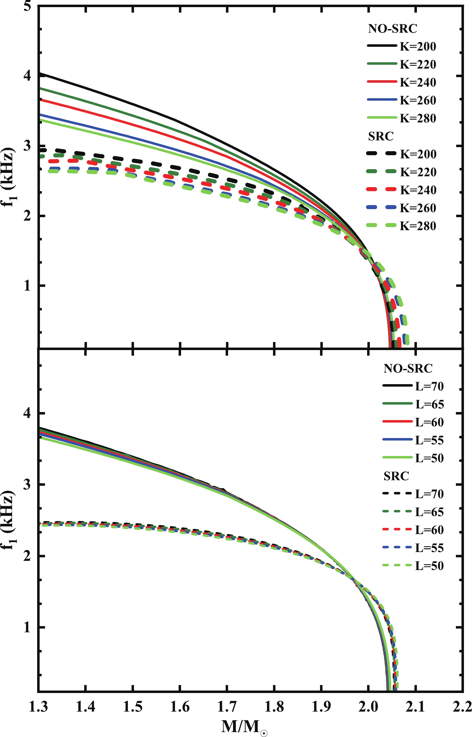
Figure 8. (color online) The relationship between NS's mass and fundamental radial frequency with different parameters. The solid lines and dotted lines represent no-SRC and SRC respectively.
As mentioned in Fig. 7, we can also understand this conclusion from another aspect. Fig. 2 has shown that SRC has a larger NS radius therefore a smaller average density, since the non-radial oscillations are accompanied with the radial ones [53], resulting the radial frequency is also related to the average density like the non-radial one, i.e. low average density will give a smaller frequency. At
$ 1.4M_{\odot} $ , compared to no-SRC, SRC decreases the radial frequency$ f_{1} $ from 3.31$ \sim $ 3.75 kHz to 2.56$ \sim $ 2.90 kHz for isoscalar$ K $ showing a reduction around 0.75$ \sim $ 0.85 kHz, while decreases from 3.59 kHz to 2.78 kHz for isovector$ L $ showing a reduction of approximately 0.81 kHz. However, as the mass of the NS increases, the SRC effect will gradually become ineffective, because we have introduced hyperon degrees of freedom in this article. The internal high density will transform nucleons into hyperons, which will further compress the number of nucleon short-range correlations. Moreover, because Fig. 2 has shown that SRC can yield a larger maximum mass, as the frequency decreases, before approaching the maximum mass, there must be a transition that makes the radial frequency given by SRC exceed the one by no-SRC, being a unique feature for radial vibration after considering SRC. The position of this transition is roughly at$ 2M_{\odot} $ ; therefore, in Fig. 8, we observe that the radial frequency given by SRC at the low mass is lower, whereas at the high mass the opposite is true. When compared to low-mass NSs, this difference is still quite small.Additionally, we calculated the other highly excited modes of
$ 1.4M_{\odot} $ and$ 2M_{\odot} $ and listed their corresponding frequencies in Table 3. After considering the SRC effect, one can observe that other modes have the similar conclusion in the fundamental mode$ f_{1} $ , i.e. the corresponding radial frequency will decrease and the SRC effect will gradually become ineffective roughly near$ 2M_{\odot} $ . To illustrate the latter, we have plotted the radial eigenfunctions of different modes in Fig. 9, which shows that the difference between the eigenfunctions given by SRC and no-SRC at$ 2M_{\odot} $ are very small. This result will be very useful. On one hand, for the low-mass NS composed of nucleon degrees of freedom in$ \beta $ equilibrium, a large number of SRC nucleons will lead to a significant reduction in the radial frequency. This reduction can be regarded as direct evidence of nucleon-nucleon short range correlation, which could be tested by future observation from the new generation of highly sensitive gravitational wave detectors such as Cosmic Explorer or Einstein Telescope [148–150]. On the other hand, for massive ones near$ 2M_{\odot} $ , SRC can be used as a probe for the structure inside the NSs. If the observed values are comparable with our results, we can at least believe that there must be other degrees of freedom in the NS besides the nucleons. These degrees of freedom will weaken the short-range correlation between the nuclei and may be the hyperon components, or the quark components,K meson condensations, etc. Although it is impossible to determine the specific matter, the existence of other degrees of freedom will inevitably lead to a decrease in the number of SRC nucleons. CASE $ 1.4M_{\odot} $ 

$ 2M_{\odot} $ 

$f_{1} /{\rm{kHz} }$ 

$f_{2} /{\rm{kHz} }$ 

$f_{3}/{\rm{kHz} }$ 

$f_{4} /{\rm{kHz} }$ 

$f_{1}/{\rm{kHz} }$ 

$f_{2} /{\rm{kHz} }$ 

$f_{3}/{\rm{kHz} }$ 

$f_{4}/{\rm{kHz} }$ 

No.1 2.902[3.751] 5.890[6.550] 7.713[8.768] 9.757[10.929] 1.435[1.432] 4.908[4.905] 6.219[6.218] 7.990[7.989] No.2 2.891[3.637] 5.791[6.351] 7.656[8.556] 9.651[10.760] 1.434[1.432] 4.906[4.902] 6.218[6.216] 7.987[7.988] No.3 2.872[3.591] 5.702[6.301] 7.511[8.471] 9.528[10.628] 1.433[1.431] 4.905[4.901] 6.215[6.215] 7.985[7.986] No.4 2.605[3.497] 5.599[6.213] 7.391[8.399] 9.398[10.513] 1.432[1.430] 4.902[4.900] 6.212[6.212] 7.982[7.983] No.5 2.561[3.315] 5.410[6.017] 7.273[8.210] 9.209[10.398] 1.431[1.430] 4.901[4.898] 6.210[6.211] 7.981[7.982] No.3 2.872[3.591] 5.702[6.301] 7.511[8.471] 9.528[10.628] 1.433[1.431] 4.905[4.901] 6.215[6.215] 7.985[7.986] No.6 2.875[3.602] 5.709[6.327] 7.519[8.490] 9.534[10.657] 1.433[1.431] 4.907[4.903] 6.218[6.221] 7.991[7.988] No.7 2.879[3.618] 5.711[6.358] 7.522[8.521] 9.539[10.692] 1.435[1.432] 4.910[4.906] 6.221[6.229] 7.994[7.995] No.8 2.880[3.635] 5.719[6.392] 7.528[8.539] 9.546[10.753] 1.436[1.432] 4.911[4.909] 6.226[6.231] 7.996[7.997] No.9 2.881[3.652] 5.727[6.420] 7.531[8.556] 9.551[10.821] 1.436[1.433] 4.913[4.912] 6.232[6.235] 7.999[8.003] Table 3. Radial oscillation frequencies
$ f_{n}(n=1, 2, 3, 4) $ of$ 1.4M_{\odot} $ and$ 2M_{\odot} $ using different parameters. The frequency unit is kHz, and the square brackets indicate that there is no-SRC effect.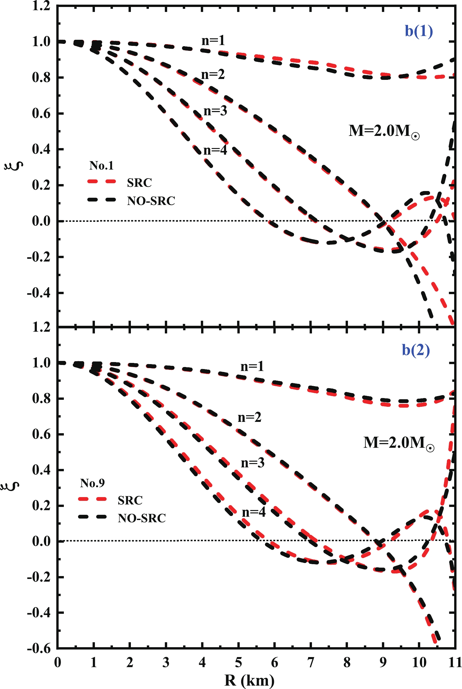
Figure 9. (color online) Relationship between NS radius and
$ \xi $ perturbation eigenfunction in different modes for$ 2M_{\odot} $ . The red and black dotted lines represent no-SRC and SRC, respectively. -
In this study, we evaluate the influence of the nucleon-nucleon short range correlation (SRC) on the static spherically symmetric neutron stars (NSs) from the perspectives of radial oscillations and nonradial oscillations. We revised the energy-momentum expression and nucleon coupling parameters in the relativistic mean field theory after considering the SRC effect. We also considered the hyperon degrees of freedom inside the NS and selected the
$SU$ (3) model to construct the coupling parameters that can meet the multi-messenger astronomy constraints from NICER, GW170817, and observation of massive NSs. Through numerical calculation, we made the following conclusions:(1) The NS's mass-radius relationship obtained by the
$SU$ (3) group under the SRC effect can effectively meet the results of multi-astronomical messenger observations and to a certain extent avoid the hyperon puzzle. Additionally, as shown in Fig. 2, the SRC effect will increase the maximum mass and radius of the NS.(2) The SRC effect can significantly increase the dimensionless tidal deformability values in the vicinity of
$ 1.4M_{\odot} $ , and compared to no-SRC, it is approximately$ 200_{-10}^{+25} $ higher.(3) For non-radial oscillations, the
$ f $ -mode frequency increases with the mass, and the SRC effect decreases the$ f $ -mode frequency by$ 0.2\sim0.3 $ kHz (approximately 7.35%~11.57% reduction). We refit the linear relationship between the average density and$ f $ -mode frequency, and demonstrate a parameter-independent relationship for on-SRC with$ f({\rm{kHz}}) = (1.28162\pm 0.03127)+(1.20736\pm $ $ 0.03019)\sqrt{\dfrac{\bar{M}}{\bar{R}^{3}}} $ in the 90% credible intervals and for SRC with$ f({\rm{kHz}}) = (0.56062\pm 0.00972)+(1.77151\pm 0.00918) $ $ \sqrt{\dfrac{\bar{M}}{\bar{R}^{3}}} $ .(4) For the radial oscillations, the fundamental frequency decreases with the NS mass, and drops sharply to zero when the mass gradually approaches the maximum mass. Combining the characteristics of the non-radial frequencies, we can determine the maximum mass of NSs.
(5) After the introduction of SRC, the radial frequency
$ f_{1} $ is decreased by approximately 0.75~0.85 kHz (approximately 22.5%~22.66% reduction) at$ 1.4M_{\odot} $ , and gradually becomes ineffective for masses larger than$ 2M_{\odot} $ . Owing to characteristics of SRC's influence on the radial frequency, at low-mass NS, we expect that the SRC will be tested by future detectors such as the Cosmic Explorer or Einstein Telescope. At massive NS, the existence of other degrees of freedom will inevitably lead to a decrease in the numbers of SRC nucleons. We expect to use the SRC effect as a probe for the structure inside NSs.It should be noted that although the calculated results with the SRC show satisfactory astronomical observation, it is still highly model-dependent and the existence of the condensation of (anti) kaons and pions, and quark matter in the interior of NSs are still to be further confirmed. A reasonable introduction of these assumptions undoubtedly further deepens our understanding on the internal composition of an NS. We hope to discuss these possibilities in the near future
-
We thank professor Zi-Gao Dai for the useful discussions.
-
In this work, with the SRC-revised RMFT, we need to re-determine the value of six nucleon coupling parameters of
$ g_{\sigma N}, \; g_{\omega N}, \; g_{\rho N}, \; g_{\delta N}, \; b, \; c $ . These unknown parameters are determined through the binding energy per nucleon$ B/A $ , the incompressibility coefficient$ K $ , the nucleon effective mass$ m^{*} $ and the saturation density$ n_{0} $ . Next, we relate the coupling parameters with these saturation properties. Because we know that the energy per nucleon$ E/A $ is equal to the sum of the binding energy per nucleon$ B/A $ and nucleon mass$ m_{B} $ , i.e.$ E/A = B/A+m_{B} $ , we obtain$ \begin{aligned}[b] \frac{B}{A}+m_{B} =& \left(\frac{g_{\omega}}{m_{\omega}}\right)^{2}n_{0}+C_{1}\sqrt{k_{F}^{2}+m^{* 2}}\\& +\frac{C_{2}\lambda^{3}\sqrt{(\lambda k_{F})^{2}+m^{* 2}} }{(\lambda k_{F})^{4}}-\frac{C_{2}\sqrt{ k_{F}^{2}+m^{* 2}} }{k_{F}^{4}}\\& +\frac{1}{k_{F}^{2}}\frac{\partial C_{2}}{\partial k_{F}} \int_{k_{F}}^{\lambda k_{F}} \frac{k^{2}\sqrt{k^{2}+m^{* 2}}}{k^{4}} {\rm{d}} k , \end{aligned}\tag{A1} $

where
$ m^{*} $ represents the nucleon effective mass because the isospin-asymmetry$ \beta = 0 $ at saturation density, we have$ C_{1}^{(n)} = C_{1}^{(p)} = C_{1} $ ,$ C_{2}^{(n)} = C_{2}^{(p)} = C_{2} $ ,$ k_{F}^{(n)} = k_{F}^{(p)} = k_{F} $ . In RMFT, The scalar meson$ \sigma $ meet$ \begin{aligned}[b] &\left(\frac{m_{\sigma}}{g_{\sigma}}\right)^{2}\left(m_{B}-m^{*}\right)+m_{B}\left(m_{B}-m^{*}\right)^{2} b+c\left(m_{B}-m^{*}\right)^{3}\\ =& 2\left[\frac{C_{1}}{\pi^{2}} \int_{0}^{k_{F}} \frac{m^{*} k^{2}}{\sqrt{k^{2}+m^{* 2}}} {\rm{\; d}} k+\frac{C_{2}}{\pi^{2}} \int_{k_{F}}^{\lambda k_{F}} \frac{m^{*} k^{2}}{k^{4} \sqrt{k^{2}+m^{* 2}}} {\rm{\; d}} k\right] \end{aligned}\tag{A2} $

and the energy density is expressed as
$ \begin{aligned}[b]& \frac{1}{2}\left(m_{B}-m^{*}\right)^{2}\left(\frac{m_{\sigma}}{g_{\sigma}}\right)^{2}+\frac{1}{3} m_{B}\left(m_{B}-m^{*}\right)^{3} b+\frac{1}{4}\left(m_{B}-m^{*}\right)^{4}c\\& +\frac{1}{2}\left(\frac{g_{\omega}}{m_{\omega}}\right)^{2} n_{0}^{2} = \left(B / A+m_{B}\right) n_{0}\\& -2\times\Bigg[\frac{C_{1}}{\pi^{2}} \int_{0}^{k_{F}} k^{2}\sqrt{k^{2}+m^{* 2}}{\rm{d}} k +\frac{C_{2}}{\pi^{2}} \int_{k_{F}}^{\lambda k_{F}} \frac{k^{2}\sqrt{k^{2}+m^{* 2}}}{k^{4}} {\rm{d}} k \Bigg]. \end{aligned}\tag{A3} $

The incompressibility coefficient at saturation density reads as
$ \begin{aligned}[b] K =& \left(\frac{g_{\omega}}{m_{\omega}}\right)^{2}\cdot\frac{6k_{F}^{3}}{\pi^{2}} +\Bigg(AA+BB+CC\Bigg)^{'k}\cdot3 k_{F}\\ &- \Bigg(AA+BB+CC\Bigg)^{'m*} \cdot\frac{6 k_{F}\langle\bar{\psi}\psi\rangle^{' k} }{\Bigg[\left(\dfrac{m_{\sigma}}{g_{\sigma}}\right)^{2}+2\langle\bar{\psi}\psi\rangle^{' m*} - \dfrac{{\rm d}^{2}U}{{\rm d}\sigma_{0}^{2}}\dfrac{1}{g_{\sigma}^{2}} \Bigg]}, \end{aligned}\tag{A4} $

where prime stands for the derivation of momentum
$ k $ and effective mass$ m^{*} $ , the$ AA $ ,$ BB $ ,$ CC $ and$ \langle\bar{\psi} \psi\rangle $ are expressed as$ \begin{aligned}[b] AA =& C_{1} \sqrt{k_{F}^{2}+m^{* 2}}\\ BB =& \frac{C_{2}\lambda^{3}\sqrt{(\lambda k_{F})^{2}+m^{* 2}} }{(\lambda k_{F})^{4}}-\frac{C_{2}\sqrt{ k_{F}^{2}+m^{* 2}} }{ k_{F}^{4}}\\ CC =& \frac{C'_{2}}{k_{F}^{2}} \int_{k_{F}}^{\lambda k_{F}} \frac{k^{2}\sqrt{k^{2}+m^{* 2}}}{k^{4}} {\rm{d}} k\\ \langle\bar{\psi} \psi\rangle =& \frac{2C_{1}}{\pi^{2}} \int_{0}^{k_{F}} \frac{m^{*} k^{2}}{\sqrt{k^{2}+m^{* 2}}} {\rm{\; d}} k\\ & +\frac{2C_{2}}{\pi^{2}} \int_{k_{F}}^{\lambda k_{F}} \frac{m^{*} k^{2}}{k^{4} \sqrt{k^{2}+m^{* 2}}} {\rm{\; d}} k . \end{aligned}\tag{A5} $

To determine the isovector coupling parameters
$ g_{\rho} $ and$ g_{\delta} $ , we need to know their correlations with the symmetry energy$E_{\rm sym}$ and its slope$ L $ . For the symmetry energy at saturation density$ \begin{aligned}[b] E_{\rm sym}(n_{0}) =& \frac{1}{2} \frac{\partial^{2}(E / A)}{\partial \beta^{2}}\Bigg|_{\beta = 0} = \frac{1}{2}\left[\frac{\partial^{2}(\varepsilon / n)}{\partial \beta^{2}}\right]_{\beta = 0}\\ =& E_{\rm 1sym}(n_{0})+E_{\rm 2sym}(n_{0})+E_{\rm 3sym}(n_{0}).\\ \end{aligned}\tag{A6} $

These three parts correspond to the following:
$ E_{\rm 1sym}(n_{0}) = \frac{k_{0}^{3}}{12 \pi^{2}} \frac{g_{\rho}^{2}}{m_{\rho}^{2}+2\Lambda_{\omega}\left(g_{\omega} \omega_{0}\right)^{2} g_{\rho}^{2}} \tag{A7}$

and
$ \begin{aligned}[b] E_{\rm 2sym}(n_{0}) =& \frac{k_{0}^{2}}{8\sqrt{k_{0}^{2}+m^{* 2}}}+\frac{1}{4}\sqrt{k_{0}^{2}+m^{* 2}}\\& + \Bigg[ \left(\frac{C'_{2}}{2k_{0}^{2}}\right)'\cdot\frac{k_{0}}{3}-\frac{ C'_{2}}{ k_{0}^{2}}\Bigg] \int_{k_{0}}^{\lambda k_{0}} {\rm{\; d}} k \frac{k^{2}\sqrt{k^{2}+m^{* 2}}}{k^{4}}\\& +\Bigg(\frac{C'_{2}k_{0}}{3}-C_{2}\Bigg)\Bigg(\frac{\lambda^{3} \sqrt{\left(\lambda k_{0}\right)^{2}+m^{* 2}}}{(\lambda k_{0})^{4}}- \frac{\sqrt{k_{0}^{2}+m^{* 2}}}{ k_{0}^{4}}\Bigg)\\& +\frac{k_{0}C_{2}}{6}\Bigg(\frac{\lambda^{3} \sqrt{\left(\lambda k_{0}\right)^{2}+m^{* 2}}}{(\lambda k_{0})^{4}}- \frac{\sqrt{k_{0}^{2}+m^{* 2}}}{ k_{0}^{4}}\Bigg)' \end{aligned}\tag{A8} $

and
$E_{\rm 3sym}(n_{0})$ involves the scalar-isovector meson$ \delta $ , and its expression is$ E_{\rm 3sym}(n_{0}) = -\frac{1}{2}m^{2}_{\delta}\left(\frac{\partial \delta}{\partial \beta}\right)^{2}|_{\beta = 0}\times\frac{1}{n_{0}} = -\frac{1}{2n_{0}}m^{2}_{\delta}\left(\frac{N}{M}\right)^{2} \tag{A9} $

where
$ M $ and$ N $ are expressed as:$ \begin{aligned}[b] M =& 1+\frac{3g^{2}_{\delta}}{4\pi^{2}m_{\delta}^{2}}\int_{0}^{k_{F}}\frac{2k^{4}{\rm d}{\boldsymbol{k}}}{(m^{*2}+k^{2})^{3/2}}\\& +\frac{2C_{2}g^{2}_{\delta}}{\pi^{2}m_{\delta}^{2}}\int_{k_{F}}^{\lambda k_{F}}\frac{k^{4}{\rm d}{\boldsymbol{k}}}{k^{4}(m^{*2}+k^{2})^{3/2}} \end{aligned}\tag{A10} $

and
$ \begin{aligned}[b] N = \frac{2C_{2}g_{\delta}}{\pi^{2}m_{\delta}^{2}}\int_{k_{F}}^{\lambda k_{F}}\frac{m^{*}k^{2}{\rm d}{\boldsymbol{k}}}{k^{4}\sqrt{m^{*2}+k^{2}}}-\frac{g_{\delta}}{2\pi^{2}m_{\delta}^{2}}\int_{0}^{k_{F}}\frac{m^{*}k^{2}{\rm d}{\boldsymbol{k}}}{\sqrt{m^{*2}+k^{2}}} \end{aligned} $

$ \begin{aligned}[b] \quad\quad& +\frac{3g_{\delta}}{4m_{\delta}^{2}}\frac{-m^{*}n_{0}}{\sqrt{m^{*2}+k_{F}^{2}}} -\frac{g_{\delta}C'_{2}n_{0}}{m_{\delta}^{2}k^{2}_{F}}\int_{k_{F}}^{\lambda k_{F}}\frac{m^{*}k^{2}{\rm d}{\boldsymbol{k}}}{k^{4}(m^{*2}+k^{2})^{1/2}} \\& -\frac{g_{\delta}C_{2}n_{0}}{m_{\delta}^{2}}\Bigg[\frac{m^{*}\lambda^{3}}{(\lambda k_{F})^{4}\sqrt{m^{*2}+(\lambda k_{F})^{2}}}-\frac{m^{*} }{ k_{F}^{4}\sqrt{m^{*2}+k_{F}^{2}}}\Bigg]. \end{aligned} \tag{A11}$

For the symmetry energy slope:
$ L(n_{0}) = 3n_{0}\frac{\partial E_{\rm sym}}{\partial n}\Bigg|_{n = n_{0}} = L_{1}(n_{0})+L_{2}(n_{0})+L_{3}(n_{0}) , \tag{A12}$

where
$ L_{1, 2, 3} $ is expressed as$ L_{1}(n_{0}) = 3E_{\rm 3sym} \Bigg[ 1-32\frac{g_{\omega}^{2}}{m_{\omega}^{2}} \times g_{\omega}\omega \Lambda_{\omega} \times E_{\rm 3sym} \Bigg] \tag{A13} $

and
$ \begin{aligned}[b] L_{2}(n_{0}) =& k(E_{\rm 2sym})^{'k}\\& -\frac{2k (E_{\rm 2sym})^{'m*}\langle\bar{\psi} \psi\rangle^{\prime k} }{\Bigg[ \left(\dfrac{m_{\sigma}}{g_{\sigma}}\right)^{2}+2\langle\bar{\psi} \psi\rangle^{\prime m*}+2bm(m-m^{*})+3c(m-m^{*})^{2} \Bigg]} \end{aligned}\tag{A14} $

and
$ \begin{aligned}[b] L_{3}(n_{0}) =&-3n_{0}\Bigg\{ -\frac{1}{2} m^{2}_{\delta} \frac{N^{2}}{M^{2}}\frac{1}{n_{0}^{2}}+\frac{m^{2}_{\delta}}{n_{0}}\frac{N}{M} \frac{N^{'k}M-NM^{'k}}{M^{2}}\frac{\partial k}{\partial n}\Bigg|_{n = n_{0}}\\& +\frac{m^{2}_{\delta}}{n_{0}}\frac{N}{M} \frac{N^{'m*}M-NM^{'m*}}{M^{2}}\frac{\partial m^{*}}{\partial n}\Bigg|_{n = n_{0}} \Bigg\} . \end{aligned}\tag{A15} $

In this way, the nucleon coupling parameters are successfully related to the nuclear matter properties by the equations (A1)–(A4) and (A6) and (A12). Solving these equations numerically, the six nucleon coupling parameters can be obtained.
Short-range correlation effects in neutron star's radial and non-radial oscillations
- Received Date: 2021-12-07
- Available Online: 2022-06-15
Abstract: In this study, we determine the influence of the nucleon-nucleon short range correlation (SRC) on static spherically symmetric neutron stars (NSs) from the perspectives of radial and nonradial oscillations for the first time. We revise the equation of state and coupling parameters in the relativistic mean field theory after considering the SRC effect, and select the hyperon coupling parameters as the SU(3) model. For the non-radial oscillations, the SRC effect decreases the


 DownLoad: