


 Abstract
 HTML
HTML Reference
 Related
 PDF
PDF


-
Generalized parton distributions (GPDs) [1–4] include a wealth of current information on three-dimensional (3D) structure of hadrons. They provide a consistent unified framework containing the elastic form factors (FFs) [5, 6] and usual parton distribution functions (PDFs) [7, 8], and offering more information. GPDs emerge in the calculation of hard exclusive process such as deeply virtual Compton scattering (DVCS) [9–11], deeply virtual meson production (DVMP) [12] and time-like Compton scattering (TCS) [13]. Factorization allows us to express the amplitudes of these reactions as the convolution of a hard scattering kernel and a soft matrix element of quark and/or gluon fields which consist in the GPDs [14, 15]. GPDs are the only experimental way to indirectly probe the energy-momentum tensor (EMT). The relationship between the EMT and GPDs can be used to obtain the message about the mechanical properties of partonic systems, like pressure distributions inside the nucleon [16]. In addition, the Mellin moments of GPDs contain the information of electromagnetic and gravitational properties of hadrons. The gravitational properties yield additional insights on the way that angular momentum and mass are distributed among the quarks and gluons inside the hadron, thus addressing deep issues about the spin [17] and mass [18, 19] decompositions of hadrons straightforwardly. Through the two-dimensional Fourier transformation, GPDs become spatial light cone distributions of partons in impact parameter space [20].
We are interested in pion GPDs [21–28], Refs. [29–31] suggest the chances to obtain experimental access to pion GPDs. Pion GPDs are studied both on transverse [32] as well as Euclidean [33] lattices.
At present, it is impossible to determine the GPDs from QCD directly, effective models have been applied to supply estimates which should serve to direct future experiments. However, up to now, it is still a challenge to model GPDs and various methods have been developed [34–46]. The calculation of GPD models should satisfy the theoretical constraints required by the symmetries of QCD.
In this study, we use the Nambu-Jona-Lasinio (NJL) [47–50] model to investigate the pion GPDs using different regularization schemes. The NJL model is used in many fields, it has an effective Lagrangian of relativistic fermions interacting through local fermion-fermion couplings. Besides, it keeps the fundamental symmetries of QCD, of which the most important one is chiral symmetry. A fly in the ointment is that NJL is non-renormalizable, so we need a regularization scheme to totally define the model. Several regularization methods are commonly used, such as the 3D momentum non-covariant cutoff scheme, the four- dimensional (4D) momentum cutoff scheme [51–54], proper time (PT) regularization scheme [26, 27, 53, 55–60], the Pauli-Villars (PV) scheme [61, 62]. The latter three have the attractive character of being Lorentz invariant. The 3D cutoff scheme is the most popular method in this model and a lot of works have been done in this way [63], when the model is applied to thermodynamics, most authors prefer to regularize the integrals by a (sharp or smooth) three-momentum cutoff [50, 64–67]. The 4D cutoff method preserves the Lorentz symmetry in which space and time are treated on equal footing. The PV regularization is based on the subtraction of the amplitude considering the virtually heavy particle to suppress the nonphysical high energy contribution coming from the loop integrals. The PT regularization makes integrals finite through the exponentially dumping factor, in this regularization scheme we introduce the infrared cutoff
$ \Lambda_{\rm{IR}} $ to mimic confinement.We use the four regularization schemes in this paper, each of them have their advantages and disadvantages, we want to see the difference of pion GPDs in different regularization schemes.
This paper is organized as follows: Sec. II briefly introduces the NJL model and then demonstrates the definition and calculation of the pion GPDs. Sec. III gives the results of pion GPDs using different regularization schemes. Sec. IV gives a summary and conclusion.
-
The
$SU $ (2) flavor NJL Lagrangian is$ \begin{aligned}[b] {\cal{L}}=&\bar{\psi }\left({\rm i}\gamma ^{\mu }\partial _{\mu }-\hat{m}\right)\psi\\&+\frac{1}{2} G_{\pi }\left[\left(\bar{\psi }\psi\right)^2-\left( \bar{\psi }\gamma _5 \vec{\tau }\psi \right)^2\right]-\frac{1}{2}G_{\omega}\left(\bar{\psi }\gamma _{\mu}\psi\right)^2\\ &-\frac{1}{2}G_{\rho}\left[\left(\bar{\psi }\gamma _{\mu} \vec{\tau } \psi\right)^2+\left( \bar{\psi }\gamma _{\mu}\gamma _5 \vec{\tau } \psi \right)^2\right], \end{aligned} $

(1) where
$ \vec{\tau} $ are the Pauli matrices represent isospin and the current quark mass matrix$ \hat{m}={\rm{diag}}\left(m_u,m_d\right) $ . In the isospin symmetry,$ m_u = m_d =m $ .$ G_{\pi} $ ,$ G_{\omega} $ , and$ G_{\rho} $ are the four-fermion coupling constants in each chiral channel.The fundamental quark-antiquark interaction kernel is defined as [68]
$ \begin{aligned}[b] {\cal{K}}_{\alpha\beta,\gamma\delta}=&\sum\limits_{\Omega}{\rm{K}}_{\Omega}\Omega_{\alpha\beta}\bar{\Omega}_{\gamma\delta}\\ =&2{\rm i}G_{\pi}[(1)_{\alpha\beta}(1)_{\gamma\delta}-(\gamma_5\tau_i)_{\alpha\beta}({\gamma_5\tau_i})_{\gamma\delta}]\\ &-2{\rm i}G_{\rho}[(\gamma_{\mu}\tau_i)_{\alpha\beta}(\gamma_{\mu}\tau_i)_{\gamma\delta}+(\gamma_{\mu}\gamma_5\tau_i)_{\alpha\beta}(\gamma_{\mu}\gamma_5\tau_i)_{\gamma\delta}]\\ &-2{\rm i}G_{\omega}(\gamma_{\mu})_{\alpha\beta}(\gamma_{\mu})_{\gamma\delta}, \end{aligned} $

(2) where the label represents the Dirac, color, and isospin indices.
The dressed-quark propagator is obtained by solving the gap equation
$ S(k)=\frac{1}{{\notk}-M+ {\rm i} \varepsilon}, $

(3) we obtained a constant dressed-quark mass M which satisfied
$ M=m+12 {\rm i} G_{\pi}\int \frac{{\rm{d}}^4l}{(2 \pi )^4}{\rm{tr}}_{\rm D}[S(l)], $

(4) where the trace is over Dirac indices. When the effective coupling strength
$ G_{\pi} $ is larger than$ G_{\rm{critical}} $ , dynamical chiral symmetry breaking (DCSB) occurs and gives a nontrivial solution$ M > 0 $ . The quark charge operator in the NJL model is$ \hat Q = \left( {\begin{array}{*{20}{c}} {{e_u}}&0\\ 0&{{e_d}} \end{array}} \right) = \left(\frac{1}{6} + \frac{{{\tau _3}}}{2}\right), $

(5) where
$ e_u $ and$ e_d $ are the u and d quark charges, respectively. This means that the quark-photon vertex has both an isovector and an isoscalar component, now the dressed quark-photon vertex can be expressed as$ \Lambda_{\gamma Q}^{\mu}(p',p)=\frac{1}{6}\Lambda_{\omega}^{\mu}(p',p)+\frac{\tau_3}{2}\Lambda_{\rho}^{\mu}(p',p), $

(6) the effective vertex
$ \Lambda_i^{\mu}(Q^2)=\gamma^{\mu}F_{1i}(Q^2)+\frac{\sigma^{\mu\nu}q_{\nu}}{2M}F_{2i}(Q^2), $

(7) where
$ i=(\omega,\rho) $ . This vertex has the same form as the electromagnetic current for an on-shell spin-$ \dfrac{1}{2} $ fermion. For a point-like quark$ F_{1i}(Q^2)=1 $ and$ F_{2i}(Q^2) =0 $ . The inhomogeneous Bethe-Salpeter equation (BSE) for the quark-photon vertex is depicted in Fig. 1,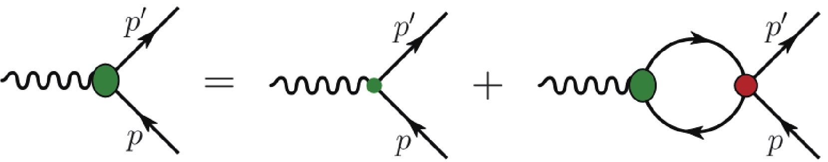
Figure 1. (color online) Inhomogeneous BSE whose solution gives the quark-photon vertex, represented as the large-shaded oval.
$ \begin{aligned}[b] \Lambda_{\gamma Q}^{\mu}(p',p)=&\gamma^{\mu}\left(\frac{1}{6}+\frac{\tau_3}{2}\right)+\sum\limits_{\Omega}{\rm{K}}_{\Omega}\Omega\int \frac{{\rm d}^4k}{(2\pi)^4}\\ & \times {\rm{tr}}[\bar{\Omega} S(k+q)\Lambda_{\gamma Q}^{\mu}(k+q,k)S(k)], \end{aligned} $

(8) where
$ \sum_{\Omega}{\rm{K}}_{\Omega}\Omega_{\alpha\beta} \bar{\Omega}_{\gamma\delta} $ stand for the interaction kernels in Eq. (2), only the isovector-vector,$-2{\rm i}G_{\rho}(\gamma_{\mu}\vec{\tau })_{\alpha\beta}(\gamma_{\mu}\vec{\tau })_{\gamma\delta}$ , and isoscalar-vector$-2{\rm i}G_{\omega}(\gamma_{\mu})_{\alpha\beta}(\gamma_{\mu})_{\gamma\delta}$ terms can contribute.From the inhomogeneous BSE, the dressed-quark FFs, associated with the electromagnetic current of Eq. (7), are
$ F_{1i}(Q^2)=\frac{1}{1+2G_i \Pi_{\rm{VV}}(Q^2)},\quad \quad F_{2i}(Q^2)=0. $

(9) The vector bubble diagram has the form
$ \begin{aligned}[b] & \Pi_{\rm{VV}}(q^2)\left(g^{\mu\nu}-\frac{q^{\mu}q^{\nu}}{q^2}\right)\delta_{ij}\\ =&3{\rm i}\int \frac{{\rm d}^4k}{(2\pi)^4}{\rm{tr}}[\gamma^{\mu}\tau_iS(k)\gamma^{\nu}\tau_jS(k+q)]. \end{aligned} $

(10) The pion vertex function, in the light-cone normalization, is given by
$ \Gamma_{\pi}^{i}=\sqrt{Z_{\pi}}\gamma_5\tau_i ,$

(11) where
$ Z_{\pi} $ is the effective meson-quark-quark coupling constant. The pseudoscalar bubble diagram$ \Pi_{\rm{PP}}(q^2)\delta_{ij}=3{\rm i}\int \frac{{\rm{d}}^4k}{(2 \pi )^4}{\rm{tr}}[\gamma^5\tau_iS(k)\gamma^5\tau_jS(k+q)], $

(12) where the traces are over Dirac and isospin indices. Meson masses are then defined by the pole in the two body t matrix, respectively. The normalization factor is determined by
$ Z_{\pi}^{-1}=-\frac{\partial}{\partial q^2}\Pi_{\rm{PP}}(q^2)|_{q^2=m_{\pi}^2}. $

(13) The pion decay constant are defined as Ref. [49]
$ \begin{aligned}[b] f_{\pi}=& \int \frac{{\rm{d}}^4k}{(2 \pi )^4}\frac{-4{\rm i}N_c\sqrt{Z_{\pi}}M}{\left(\left(k+\dfrac{p}{2}\right)^2-M^2\right)\left(\left(k-\dfrac{p}{2}\right)^2-M^2\right)}\\=&\int_0^1 {\rm{d}}x \int \frac{{\rm{d}}^4k}{(2 \pi )^4}\frac{-4{\rm i}N_c\sqrt{Z_{\pi}}M }{(k^2-x(x-1)m_{\pi}^2-M^2)}, \end{aligned} $

(14) in all these regularization schemes, there are two parameters, the coupling constant
$ G_{\pi} $ and the cutoff Λ are fixed by the pion decay constant$ f_{\pi} $ and quark condensate$ \langle \bar{u}u\rangle=\langle \bar{d}d\rangle $ .$ G_{\omega} $ and$ G_{\rho} $ are determined by$ m_{\omega}=0.782 $ GeV,$ m_{\rho}=0.770 $ GeV through$ 1+2G_i \Pi_{\rm{VV}} (m_i^2)=0 $ , where$ i=(\omega,\rho) $ .We will use the notations and formulas in the appendix in the following.
-
The pion GPDs are given in Fig. 2, where p is the incoming and
$ p' $ the outgoing pion momentum, here we use the symmetry notation, the kinematics and associated quantities are defined as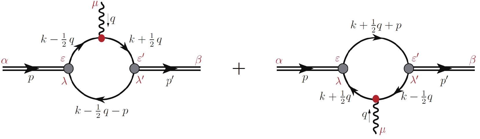
Figure 2. (color online) Pion GPDs diagrams.
$ p'^{2}=p^2=m_{\pi}^2, \quad \quad t=q^2=(p'-p)^2=-Q^2, $

(15) $ \xi=\frac{p^+-p'^+}{p^++p'^+},\quad P=\frac{p^++p'^{+}}{2}, \quad n^2=0, $

(16) ξ is the skewness parameter, in the light-cone coordinate
$ v^{\pm}=(v^0\pm v^3), \quad {\bf{v}}=(v^1,v^2), $

(17) for any four-vector, n is the light-cone four-vector
$ n=(1,0,0,-1) $ ,$ v^+ $ in the light-cone coordinate is defined as$ v^+=v\cdot n. $

(18) GPDs are defined as the Fourier transform of a non-perturbative matrix element of a quark operators depending on a light-like distance,
$ \begin{aligned}[b] H(x,\xi,t)=&\frac{1}{2}\int \frac{{\rm{d}}z^-}{2\pi}{\rm e}^{\frac{\rm i}{2}x(p^++p'^+)z^-}\\ &\times \langle p'|\bar{q}\left(-\frac{1}{2}z\right)\gamma^+q\left(\frac{1}{2}z\right)|p\rangle \mid_{z^+=0,{\boldsymbol{z}}={\bf{0}},} \end{aligned} $

(19) $ \begin{aligned}[b] \frac{P^+q^j-P^jq^+}{P^+m_{\pi}}E(x,\xi,t)=&\frac{1}{2}\int \frac{{\rm{d}}z^-}{2\pi}{\rm e}^{\frac{\rm i}{2}x(p^++p'^+)z^-}\\ &\times \langle p'|\bar{q}\left(-\frac{1}{2}z\right){\rm i}\sigma^{+j}q\left(\frac{1}{2}z\right)|p\rangle \mid_{z^+=0,{\boldsymbol{z}}={\bf{0}},} \end{aligned} $

(20) where x is the longitudinal momentum fraction. The first equation corresponds to the vector or no spin flip GPD, the second equation corresponds to tensor or spin flip GPD.
The insert operators in Fig. 2 have the form
$ \bullet_1 =\gamma^+\delta\left(x-\frac{k^+}{P^+}\right)\,, \tag{21a}$

$ \bullet_2 ={\rm i}\sigma^{+j} \delta\left(x-\frac{k^+}{P^+}\right),\tag{21b} $

$ \bullet_1 $ for vector GPD and$ \bullet_2 $ for tensor GPD.In the NJL model, GPDs are defined as
$ \begin{aligned}[b] H^a\left(x,\xi,t\right) =&2{\rm i} N_c Z_{\pi} \int \frac{{\rm{d}}^4k}{(2 \pi )^4}\delta_n^x (k)\\ &\times {\rm{tr}}_{\rm{D}}\left[\gamma _5 S \left(k_{+q}\right)\gamma ^+ S\left(k_{-q}\right)\gamma _5 S\left(k-P\right)\right], \end{aligned} $

(22) $ \begin{aligned}[b] \frac{P^+q^j-P^jq^+}{P^+m_{\pi}} E\left(x,\xi,t\right)=&2{\rm i} N_c Z_{\pi}\int \frac{{\rm{d}}^4k}{(2 \pi )^4}\delta_n^x (k)\\& \times {\rm{tr}}_{\rm{D}}\Big[\gamma _5 S \left(k_{+q}\right){\rm i}\sigma^{+j}S\left(k_{-q}\right) \\&\times\gamma _5 S\left(k-P\right)\Big], \end{aligned} $

(23) where
$ {\rm{tr}}_{\rm{D}} $ indicates a trace over spinor indices,$ \delta_n^x (k)=\delta (xP^+-k^+) $ ,$ k_{+q}=k+\dfrac{q}{2} $ ,$ k_{-q}=k-\dfrac{q}{2} $ .Here we use the following reduce formulas
$ p\cdot q=-\frac{q^2}{2}\,,\tag{24a} $

$ k\cdot q=\frac{1}{2} \left(D(k_{+q}^2)-D(k_{-q}^2)\right)\,,\tag{24b} $

$ k\cdot p=-\frac{1}{2} \left(D((k-P)^2)-D(k_{-q}^2)-p^2+\frac{q^2}{2}\right)\,,\tag{24c} $

$ k^2=\frac{1}{2} \left(D(k_{+q}^2)+D(k_{-q}^2)\right)+M^2-\frac{q^2}{4}, \tag{24d}$

(24d) where
$ D(k^2)=k^2-M^2 $ , applying these relationships to Eqs. (22) and (23), cancel each identical numerator and denominator factor; at last use Feynman parametrization to simplify all remaining denominators. With this method, we obtained the results.In addition to the GPDs in Fig. 2, we include the contact contribution term as shown in Fig. 2 of Ref. [45], which is plotted in Fig. 3, and this term is defined as
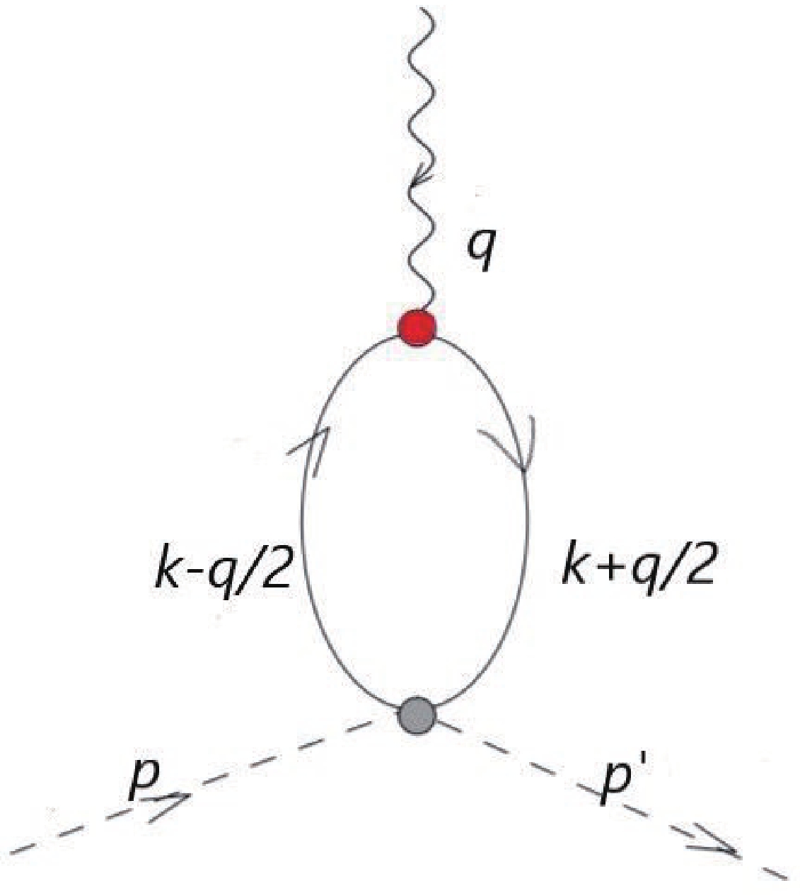
Figure 3. (color online) Contact contribution term.
$ \begin{aligned}[b] H^b\left(x,\xi,t\right)=&2{\rm i} N_c Z_{\pi}\int \frac{{\rm{d}}^4k}{(2 \pi )^4}\delta_n^x (k)\\ &\times {\rm{tr}}_{\rm{D}}\left[\gamma _5 S \left(k_{+q}\right)\gamma ^+S\left(k_{-q}\right)\gamma _5\right], \end{aligned} $

(25) In Eq. (22) we used the bare vertex
$ \gamma^+ $ , now we wanted to obtain the GPD using the dressed quark-photon vertex from the BSE. The inhomogeneous BSE for the quark-photon vertex is depicted in Fig. 1, on the right-hand side, there are two diagrams, the first diagram corresponds to the bare quark-photon vertex, using this vertex we obtained the GPD in Eq. (22), using vertex of the second diagram we obtained the term$ H^c(x,\xi,t) $ , adding the two terms together we obtained the GPD which corresponded to the dressed quark-photon vertex on the left-hand side.$ H^c $ is depicted in Fig. 4, after some calculation, we obtained the final form of$ H^c $ 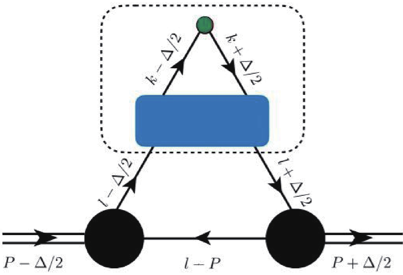
Figure 4. (color online) Diagram for
$H^c(x,\xi,t)$ . The dash line boxed area represents the dressed vertex$\Gamma^+$ .$ H^c\left(x,\xi,t\right)=F^{\alpha}(t)P^{\alpha}(x,\xi,t), $

(26) where
$ F^{\alpha}(t)=(p^{\alpha}+p^{'\alpha})F(t) $ ,$ F(t) $ is the electromagnetic form factor, which is defined as$ \begin{aligned}[b] F^{\alpha}(t)=&2{\rm i} N_c Z_{\pi} \int \frac{{\rm{d}}^4l}{(2 \pi )^4}\\&\times {\rm{tr}}_{\rm{D}}\left[\gamma _5 S \left(l_{+q}\right)\gamma ^{\alpha} S\left(l_{-q}\right)\gamma _5 S\left(l-P\right)\right],\end{aligned} $

(27) $ P^{\alpha}(x,\xi,t) $ is defined as$ \begin{aligned}[b] P^{\alpha}(x,\xi,t)=&2{\rm i} G_{\rho}\int \frac{{\rm{d}}^4k}{(2 \pi )^4}\delta_n^x (k)\\ &\times\rm{tr}_{\rm{D}}\left[\gamma _{\alpha} S \left(k_{+q}\right)\Gamma ^+S\left(k_{-q}\right)\right], \end{aligned} $

(28) where
$ \Gamma ^+ $ is the big green vertex in the inhomogeneous BSE in Fig. 1,$ F_{1\rho}(t)\gamma^+ $ , α contract at last. -
When the initial and final hadrons have the same momentum
$ p=p' $ ,$ \xi=0 $ ,$ t=q^2=0 $ , GPD should reduce to usual pion PDF,$ u(x)=H(x,0,0), $

(29) which should satisfy
$ \int_0^1u(x) {\rm{d}}x =1. $

(30) -
GPDs are neither even nor odd of momentum fraction x, the combinations,
$ H^{I=0}(x,\xi,t)=H(x,\xi,t)-H(-x,\xi,t)\,,\tag{31a} $

$ H^{I=1}(x,\xi,t)=H(x,\xi,t)+H(-x,\xi,t),\tag{31b} $

represent the isoscalar (isovector) pion GPDs, respectively, tensor GPD
$ E(x,\xi,t) $ is resemble.Time reversal invariance requires,
$ H^u(x,\xi,t)=H^u(x,-\xi,t)\,, \tag{32a}$

$ E^u(x,\xi,t)=E^u(x,-\xi,t), \tag{32b}$

we will check this property in different regularization separately.
-
The Mellin moments of GPDs play an key role, which should satisfy the polynomiality condition
$ \int_{-1}^1 x^n H(x,\xi,t) {\rm{d}}x = \sum\limits_{i=0}^{[(n+1)/2]}\xi^{2i} A_{n+1,2i}(t)\,,\tag{33a} $

$ \int_{-1}^1 x^n E(x,\xi,t){\rm{d}}x = \sum\limits_{i=0}^{[(n+1)/2]}\xi^{2i} B_{n+1,2i}(t), \tag{33b}$

where
$ [\cdot] $ denotes the floor function,$ A_{n+1,2i}(t) $ and$ B_{n+1,2i}(t) $ are vector and tensor generalized factor factors (GFFs), respectively.For
$ n=0 $ , the FFs are ξ independent,$ \int_{-1}^1 H(x,\xi,t) {\rm{d}}x = A_{1,0}(t)\,,\tag{34a}$

$ \int_{-1}^1 E(x,\xi,t){\rm{d}}x =B_{1,0}(t),\tag{34b} $

where
$ A_{1,0}(t) $ and$ B_{1,0}(t) $ are the pion electromagnetic and tensor FFs.$ B_{1,0}(0) $ is the tensor anomalous magnetic moment for$ n=0 $ .For
$ n=1 $ :$ \begin{aligned}[b] \int_{-1}^1 x H(x,\xi,t) {\rm{d}}x=& A_{2,0}(t)+\xi^2 A_{2,2}(t)\\ =&\theta_2(t)-\xi^2\theta_1(t)\,,\end{aligned}\tag{35a}$

$ \int_{-1}^1 x E(x,\xi,t) {\rm{d}}x= B_{2,0}(t)+\xi^2 B_{2,2}(t),\tag{35b} $

where
$ \theta_1 $ relates to the quark pressure distribution and$ \theta_2 $ relates to the quark mass distribution inside the pion. The gravitational FFs satisfy the low-energy theorem$ \theta_1(0)-\theta_2(0)={\cal{O}}(m_{\pi}^2) $ [69]A light-cone energy radius was defined in relation to the generalized FF
$ A_{2,0}(Q^2) $ [70]$ \langle r_{E,LC}^2\rangle=-4\frac{\partial A_{2,0}(Q^2)}{\partial Q^2}\Big|_{Q^2=0}\,,\tag{36a}$

$ \langle r_{c,LC}^2\rangle=-4\frac{\partial F(Q^2)}{\partial Q^2}\Big|_{Q^2=0}, \tag{36b} $

the second equation is analogous to light-cone charge radius, which is used to make comparison with the light-cone energy radius.
-
The impact parameter dependent PDFs are the Fourier transform of GPDs at
$ \xi=0 $ $ q\left(x,{\boldsymbol{b}}_{\perp}^2\right)=\int \frac{{\rm{d}}^2{\boldsymbol{q}}_{\perp}}{(2 \pi )^2}{\rm e}^{-{\rm i}{\boldsymbol{b}}_{\perp}\cdot {\boldsymbol{q}}_{\perp}} H\left(x,0,-{\boldsymbol{q}}_{\perp}^2\right). $

(37) $ H(x,0,-{\boldsymbol{q}}_{\bot}^2) $ should be independent of$ -{\boldsymbol{q}}_{\bot}^2 $ when$ x\rightarrow 1 $ as Ref. [71].The width distribution of u quark in the pion is defined as [71]
$ \langle {\boldsymbol{r}}_{\bot}^2\rangle_x =\frac{\displaystyle\int {\rm{d}}^2 {\boldsymbol{b}}_{\bot}{\boldsymbol{b}}_{\bot}^2u(x,{\boldsymbol{b}}_{\bot}^2)}{\displaystyle\int {\rm{d}}^2 {\boldsymbol{b}}_{\bot}u(x,{\boldsymbol{b}}_{\bot}^2)}, $

(38) when
$ x\rightarrow 1 $ , the struck quark became closer to the centre of momentum since its weight increased, this average impact parameter should be zero.The mean-squared
$ {\boldsymbol{b}}_{\bot} $ is defined as$ \langle {\boldsymbol{b}}_{\bot}^2\rangle =\int_0^1 {\rm{d}}x \int {\rm{d}}^2 {\boldsymbol{b}}_{\bot}{\boldsymbol{b}}_{\bot}^2q(x,{\boldsymbol{b}}_{\bot}^2), $

(39) then we obtained
$ \langle {\boldsymbol{b}}_{\bot}^2\rangle $ in different regularization schemes. -
The light-front transverse-spin distributions are defined as [72]
$ \rho^n\left({\boldsymbol{b}}_{\bot },{\boldsymbol{s}}_{\perp}\right) =\frac{1}{2}\left[A_{n,0}({\boldsymbol{b}}_{\bot }^2)-\frac{\varepsilon_{\bot}^{ij}{\boldsymbol{s}}_{\perp}^i{\boldsymbol{b}}_{\bot}^j}{m_{H}}B_{n,0}^{'}({\boldsymbol{b}}_{\bot }^2)\right], $

(40) where
$ m_{H} $ is the hadron mass,$ B_{n,0}^{'}({\boldsymbol{b}}_{\bot }^2)=\partial_{{\boldsymbol{b}}_{\bot }^2}B_{n,0}({\boldsymbol{b}}_{\bot }^2) $ ,$ A_{n,0}({\boldsymbol{b}}_{\bot }^2) $ and$ B_{n,0}({\boldsymbol{b}}_{\bot }^2) $ are the two-dimensional Fourier transform of$ A_{n,0}({\boldsymbol{q}}_{\bot }^2) $ and$ B_{n,0}({\boldsymbol{q}}_{\bot }^2) $ .When quark polarized in the light-front-transverse
$ +\,x $ direction, the transverse-spin density is not symmetric around$ {\boldsymbol{b}}_{\bot}=(b_x=0,b_y=0) $ anymore, the peaks shift to$ (b_x=0,b_y>0) $ [59, 60].The average transverse shifted:
$ \langle b_{\bot}^y\rangle_n^u=\frac{\displaystyle\int {\rm{d}}^2{\boldsymbol{b}}_{\bot }b_{\bot }^y \rho_u^n\left({\boldsymbol{b}}_{\bot },{\boldsymbol{s}}_{\perp}\right)}{\displaystyle\int {\rm{d}}^2{\boldsymbol{b}}_{\bot } \rho_u^n\left({\boldsymbol{b}}_{\bot },{\boldsymbol{s}}_{\perp}\right)}=\frac{1}{2m_{\pi}}\frac{B_{n,0}^u(0)}{A_{n,0}^u(0)}, $

(41) in the y direction for a transverse quark spin
$ s_{\bot} = (1, 0) $ in the x direction. -
The basic idea of PT regularization is based on [55, 56, 73].
$ \begin{aligned}[b] \frac{1}{X^n}=&\frac{1}{(n-1)!}\int_0^{\infty}{\rm{d}}\tau \,\tau^{n-1} {\rm e}^{-\tau X}\\ & \rightarrow \frac{1}{(n-1)!} \int_{1/\Lambda_{\rm{UV}}^2}^{1/\Lambda_{\rm{IR}}^2}{\rm{d}}\tau \,\tau^{n-1} {\rm e}^{-\tau X}, \end{aligned} $

(42) where the
$ 1/\Lambda_{\rm{UV}}^2 $ induces the dumping factor into the original propagator. Besides the ultraviolet cutoff, we also introduce the infrared cutoff$ \Lambda_{\rm{IR}} $ to mimic confinement. The parameters used for PT regularization scheme are demonstrated in Table 1.$\Lambda_{\rm{IR}}$ 

$\Lambda _{\rm{PT}}$ 

$M$ 

$Z_{\pi}$ 

$G_{\pi}$ 

$G_{\rho}$ 

$G_{\omega}$ 

$m_{\pi}$ 

$f_{\pi}$ 

$m$ 

$\langle\bar{u}u\rangle$ 

0.240 0.645 0.4 17.847 18.541 11.042 10.412 0.14 0.93 0.016 −(0.173)3 Table 1. Parameter set used in PT regularization scheme. The dressed quark mass and regularization parameters are in units of GeV, while coupling constant are in units of GeV−2.
Using PT regularization, the gap equation in Eq. (4) becomes
$ M =m+\frac{3G_{\pi}M}{\pi^2}\int_{1/\Lambda_{\rm{UV}}^2}^{1/\Lambda_{\rm{IR}}^2}{\rm{d}}\tau \frac{1}{\tau^2} {\rm e}^{-\tau M^2}, $

(43) the pion decay constant becomes
$ f_{\pi}^{\rm{PT}}=\frac{N_c\sqrt{Z_{\pi }}M}{4\pi ^2}\int_0^1 {\rm{d}}x\,\bar{\cal{C}}_1(\sigma_1), $

(44) the vector bubble diagram
$ \Pi_{\rm{VV}} $ is defined as$ \Pi_{\rm{VV}}^{\rm{PT}}(t)=-\frac{3 }{\pi ^2} \int_0^1{\rm{d}}x\, x (1-x) t \,\bar{\cal{C}}_1(\sigma_2). $

(45) Using PT regularization scheme, the final form of pion GPDs are
$ \begin{aligned}[b] &H_{\rm{PT}}^a\left(x,\xi,t\right) \\=&\frac{N_cZ_{\pi }}{8\pi ^2} \left[\theta_{\bar{\xi} 1}\bar{\cal{C}}_1(\sigma_3)+ \theta_{\xi 1} \bar{\cal{C}}_1(\sigma_4)+\theta_{\bar{\xi} \xi}\frac{x}{\xi }\bar{\cal{C}}_1(\sigma_5)\right]\\& +\frac{N_c Z_{\pi } }{8\pi ^2}\int_0^1 {\rm{d}}\alpha \frac{\theta_{\alpha \xi}}{\xi} (2 x m_{\pi}^2+(1-x)t) \frac{1}{\sigma_6}\bar{\cal{C}}_2(\sigma_6), \\[-15pt]\end{aligned} $

(46) $ E_{\rm{PT}}\left(x,\xi,t\right)=\frac{N_c Z_{\pi } }{4\pi ^2}\int_0^1 {\rm{d}}\alpha \frac{\theta_{\alpha \xi}}{\xi}m_{\pi}M\frac{1}{\sigma_6}\bar{\cal{C}}_2(\sigma_6), $

(47) $ H_{\rm{PT}}^b\left(x,\xi,t\right)=-\frac{N_cZ_{\pi }}{4\pi ^2} \frac{\theta_{\bar{\xi} \xi}}{\xi } M x\, \bar{\cal{C}}_1(\sigma_5), $

(48) $ H_{\rm{PT}}^c\left(x,\xi,t\right)=F_{1\rho}^{\rm{PT}}(t)A_{1,0}^{\rm{PT}}(t)\frac{N_cG_{\rho }}{4\pi ^2} \frac{\theta_{\bar{\xi} \xi}}{\xi }t\left(1-\frac{x^2}{\xi^2}\right)\bar{\cal{C}}_1(\sigma_5), $

(49) and
$ \theta_{\bar{\xi} 1}=x\in[-\xi, 1]\,,\tag{50a} $

$ \theta_{\xi 1}=x\in[\xi, 1]\,, \tag{50b}$

$ \theta_{\bar{\xi} \xi}=x\in[-\xi, \xi]\,,\tag{50c}$

$ \theta_{\alpha \xi}=x\in[\alpha (\xi +1)-\xi , \alpha (1-\xi)+\xi ]\cap x\in[-1,1], \tag{50d}$

where θ is the step function, x only existed in the corresponding region. Thus,
$ \theta_{\bar{\xi} \xi}/\xi=\Theta(1-x^2/\xi^2) $ , where$ \Theta(x) $ is the Heaviside function, and$ \theta_{\alpha \xi}/\xi=\Theta((1-\alpha)^2- $ $ (x-\alpha)^2/ \xi^2)\Theta(1-x^2) $ . These results are in the region$ \xi > 0 $ , under$ \xi \rightarrow -\xi $ :$ \theta_{\bar{\xi} 1} \leftrightarrow \theta_{\xi 1} $ ; and$ \theta_{\bar{\xi} \xi}/\xi $ ,$ \theta_{\alpha \xi}/\xi $ are invariant. The dressed vector GPDs are$ H_{\rm{PT}}^D\left(x,\xi,t\right)=H_{\rm{PT}}^a\left(x,\xi,t\right)+H_{\rm{PT}}^b\left(x,\xi,t\right)+H_{\rm{PT}}^c\left(x,\xi,t\right). $

(51) We plot the diagrams of vector and tensor GPDs using PT regularization in Figs. 5 and 6. From the diagrams we saw,
$ H^a\left(x,\xi,0\right)=0 $ when$ x<-\xi $ , GPDs were continuous but not differentiable at$ x =\pm \, \xi $ except$ \xi=0 $ [60], tensor GPD was similar. When considering the dressed quark-photon vertex and the contact contribution term, vector GPD would be not continuous at$ x =\pm \, \xi $ , from Fig. 6 we saw that the discontinuity came from the contact contribution term.
Figure 5. (color online) Pion GPDs (left panel: vector GPD, right panel: tensor GPD) at
$ \xi=0.5 $ with different t using PT regularization: black dotted line –$ t=0 $ GeV2, red line –$ t=-1 $ GeV2, blue dashed line –$ t=-5 $ GeV2, purple dotdashed line –$ t=-10 $ GeV2.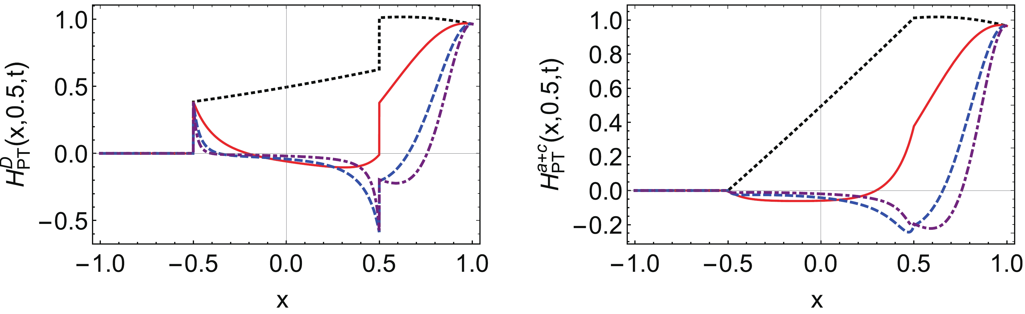
Figure 6. (color online) Pion GPDs (left panel:
$ H_{\rm{PT}}^D $ , right panel:$ H_{\rm{PT}}^a+H_{\rm{PT}}^c $ ) at$ \xi=0.5 $ with different t using PT regularization: black dotted line –$ t=0 $ GeV2, red line –$ t=-1 $ GeV2, blue dashed line –$ t=-5 $ GeV2, purple dotdashed line –$ t=-10 $ GeV2. -
In the forward limit
$ u_{\rm{PT}}(x)=\frac{3Z_{\pi }}{4\pi ^2}\bar{\cal{C}}_1(\sigma_1) +\frac{3Z_{\pi }}{2\pi ^2} x(1-x) m_{\pi}^2 \frac{\bar{\cal{C}}_2(\sigma_1)}{\sigma_1}, $

(52) which satisfies
$ \int_0^1 u(x){\rm{d}}x=1. $

(53) This PDF, varied around 1, and only changed a little with x. In the chiral limit
$ m_{\pi}=0 $ , pion PDF$ q(x)=1 $ , Refs. [27, 74, 75]. When$ m_{\pi}\neq 0 $ , our results showed pion PDF$ q(x)\approx 1 $ , it fluctuated around 1. Ref. [75] plotted pion PDF with different values of$ m_{\pi} $ . For comparison, we plotted the diagrams of u quark PDFs of pion with different values of$ m_{\pi} $ in Fig. 7.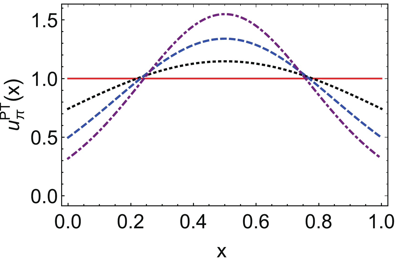
Figure 7. (color online) Pion u quark PDF with different values of
$ m_{\pi} $ using PT regularization scheme: red line –$ m_{\pi}=0 $ GeV, black dotted line –$ m_{\pi}=0.4 $ GeV, blue dashed line –$ m_{\pi}=0.6 $ GeV, purple dotdashed line –$ m_{\pi}=0.75 $ GeV. -
The dressed form factors
$ \begin{aligned}[b] A_{1,0}^{D,\rm{PT}}(t)=& \int_{-1}^1 H_{\rm{PT}}^D\left(x,\xi,t\right){\rm{d}}x\\ =&\int_{-1}^1 H_{\rm{PT}}^a\left(x,\xi,t\right){\rm{d}}x\\ &+F_{1\rho}^{\rm{PT}}(t)A_{1,0}^{\rm{PT}}(t)\int_{-1}^1 P\left(x,\xi,t\right){\rm{d}}x\\ =&A_{1,0}^{\rm{PT}}(t)-F_{1\rho}^{\rm{PT}}(t)A_{1,0}^{\rm{PT}}(t)2G_{\rho}\Pi_{\rm{VV}}(t)\\ =&A_{1,0}^{\rm{PT}}(t)F_{1\rho}^{\rm{PT}}(t), \end{aligned} $

(54) where
$ H_{\rm{PT}}^b(x,\xi,t) $ is an odd function of x, so$ \int_{-1}^1 H_{\rm{PT}}^b(x,\xi,t){\rm{d}}x=0, $

(55) however,
$ \begin{aligned}[b]& \int_{-1}^1 x H_{\rm{PT}}^b(x,\xi,t){\rm{d}}x\\ =& -\xi^2 \frac{N_c Z_{\pi } }{\pi ^2} \int_0^1 {\rm{d}}x \,M x (1-2x) \bar{\cal{C}}_1(\sigma_2),\end{aligned} $

(56) so it supplied
$ A_{2,2} $ , the final form of quark pressure distribution was$ A_{2,2}^D=A_{2,2}+A_{2,2}^b $ .$ \begin{aligned}[b] A_{1,0}^{\rm{PT}}(t)=&\frac{N_cZ_{\pi } }{4\pi^2}\int_0^1 {\rm{d}}x\,\bar{\cal{C}}_1(\sigma_1)\\ &+\frac{N_cZ_{\pi }}{4\pi^2} \int_0^1 {\rm{d}}x \int_0^{1-x}{\rm{d}}y \\ &\times (2m_{\pi }^2-(x+y)(2m_{\pi }^2-t)) \frac{1}{\sigma_7}\bar{\cal{C}}_2(\sigma_7), \end{aligned} $

(57) $ B_{1,0}^{\rm{PT}}(t) =\frac{ N_c Z_{\pi } }{2\pi ^2} \int _0^1{\rm{d}}x \int _0^{1-x}{\rm{d}}y \frac{M m_{\pi}}{\sigma_7}\bar{\cal{C}}_2(\sigma_7). $

(58) $ \begin{aligned}[b] A_{2,0}^{\rm{PT}}(t)=&\frac{N_cZ_{\pi }}{8\pi ^2}\int_0^1 {\rm{d}}x\,\bar{\cal{C}}_1(\sigma_1) \\ &+\frac{N_c Z_{\pi }}{4\pi ^2} \int_0^1 {\rm{d}}x \int_0^{1-x} {\rm{d}}y\frac{1}{\sigma_7}\bar{\cal{C}}_2(\sigma_7) \\ &\times (2 m_{\pi }^2 (1-x-y)^2+t (1-x-y) (x+y)), \end{aligned} $

(59) $ \begin{aligned}[b] A_{2,2}^{\rm{PT}}(t)=&-\frac{N_cZ_{\pi }}{4\pi ^2}\int_0^1 {\rm{d}}x\,(1-x)\bar{\cal{C}}_1(\sigma_1)\\ &-\frac{N_c Z_{\pi } }{2\pi ^2} \int_0^1 {\rm{d}}x \,x (1-2x) \bar{\cal{C}}_1(\sigma_2)\\ &-\frac{N_c Z_{\pi } }{4\pi^2} \int_0^1 {\rm{d}}x \frac{ (1-x ) \left(2 m_{\pi }^2-t\right)}{t}\bar{\cal{C}}_1(\sigma_1)\\ &+\frac{N_c Z_{\pi }}{4\pi^2}\int_0^1 {\rm{d}}x \int_0^{1-x} {\rm{d}}y \frac{\left(2 m_{\pi }^2-t\right)}{t }\bar{\cal{C}}_1(\sigma_7), \end{aligned} $

(60) $ \begin{aligned}[b] B_{2,0}^{\rm{PT}}(t)=&\frac{N_c Z_{\pi} }{2\pi ^2} \int_0^1 {\rm{d}}x \int_0^{1-x} {\rm{d}}y \\&\times m_{\pi}M (1-x-y)\frac{1}{\sigma_7}\bar{\cal{C}}_2(\sigma_7), \end{aligned} $

(61) $ B_{2,2}(t) $ is zero. -
In the PT regularization scheme
$ \begin{aligned}[b] u^{\rm{PT}}\left(x,{\boldsymbol{b}}_{\perp}^2\right) =&\frac{N_cZ_{\pi }}{4\pi ^2} \int \frac{{\rm{d}}^2{\boldsymbol{q}}_{\perp}}{(2 \pi )^2}{\rm e}^{-{\rm i}{\boldsymbol{b}}_{\perp}\cdot {\boldsymbol{q}}_{\perp}} \bar{\cal{C}}_1(\sigma_1) \\& +\frac{N_cZ_{\pi }}{32\pi ^3}\int_0^{1-x} {\rm{d}}\alpha \int {\rm{d}}\tau \\& \times \frac{(x-1) \left(4-\dfrac{{\boldsymbol{b}}_{\perp}^2}{\alpha (1-\alpha -x)\tau }\right)+8 \alpha x (1-\alpha-x)\tau m_{\pi }^2 }{4 \alpha ^2 \tau ^2 (1-\alpha-x)^2 } \\& \times {\rm e}^{ -\tau \left(M^2-x \left(1-x\right) m_{\pi}^2\right)} {\rm e}^{-\frac{{\boldsymbol{b}}_{\perp}^2}{4\tau \left(1-\alpha-x\right) \alpha}}, \end{aligned} $

(62) $ \begin{aligned}[b] u_T^{\rm{PT}}\left(x,{\boldsymbol{b}}_{\perp}^2\right) =&\frac{N_cZ_{\pi }}{16\pi^3}\int_0^{1-x} {\rm{d}}\alpha \int {\rm{d}}\tau \frac{m_{\pi}M }{\alpha\left(1-\alpha-x\right)\tau }\\&\times {\rm e}^{- \frac{{\boldsymbol{b}}_{\perp}^2}{4\tau (1-\alpha-x)\alpha}}{\rm e}^{-\tau \left(M^2-x \left(1-x\right) m_{\pi}^2\right)}, \end{aligned} $

(63) for
$ u^{\rm{PT}}\left(x,{\boldsymbol{b}}_{\perp}^2\right) $ , when integrating$ {\boldsymbol{b}}_{\perp} $ we obtained PDF$ u_{\rm{PT}}(x) $ in Eq. (52). We plot the diagrams of$ x *u^{\rm{PT}}\left(x,{\boldsymbol{b}}_{\perp}^2\right) $ and$ x *u_{\rm{T}}^{\rm{PT}}\left(x,{\boldsymbol{b}}_{\perp}^2\right) $ in Fig. 8.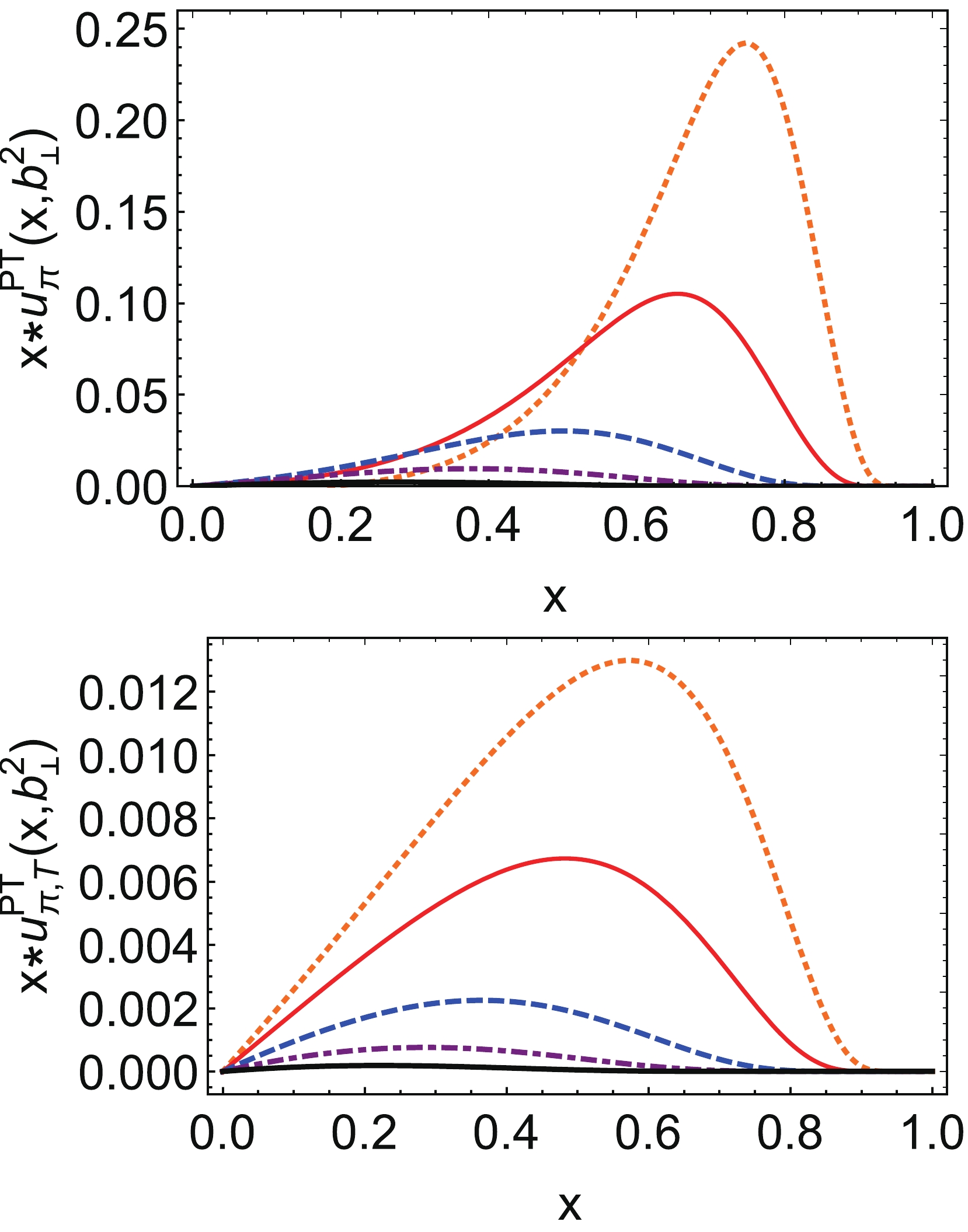
Figure 8. (color online) Impact parameter space PDFs using PT regularization scheme: left panel –
$ x*u\left(x,{\boldsymbol{b}}_{\perp}^2\right) $ , the$ \delta^2({\boldsymbol{b}}_{\perp}) $ component first line of Eq. (62) – is suppressed in the image, and right panel –$ x *u_T\left(x,{\boldsymbol{b}}_{\perp}^2\right) $ both panels with$ {\boldsymbol{b}}_{\perp}^2=0.5 $ GeV$ ^{-2} $ – orange dotted curve,$ {\boldsymbol{b}}_{\perp}^2=1 $ GeV$ ^{-2} $ – red solid curve,$ {\boldsymbol{b}}_{\perp}^2=2.5 $ GeV$ ^{-2} $ – blue dashed curve,$ {\boldsymbol{b}}_{\perp}^2=5 $ GeV$ ^{-2} $ – purple dot-dashed curve,$ {\boldsymbol{b}}_{\perp}^2=10 $ GeV$ ^{-2} $ – thick black solid curve. -
The three-momentum cutoff is after integrating out the
$ p_0 $ , a cutoff imposed on all the left integrals${\boldsymbol{p}}^2 < \Lambda^2$ , the gap equation in Eq. (4) became$ M=m-\frac{12G_{\pi}}{\pi^2}\int_0^{\Lambda_{\rm{3D}}} {\rm{d}}k\frac{k^2 M}{(k^2+M^2)^{1/2}}, $

(64) the pion decay constant became
$ f_{\pi}^{\rm{3D}}=\frac{N_c\sqrt{Z_{\pi }}M}{2\pi ^2}\int_0^1 {\rm{d}}x\int_0^{\Lambda_{\rm{3D}}}{\rm{d}}k\frac{k^2}{(k^2+\sigma_1)^{3/2}}, $

(65) the vector bubble diagram
$ \Pi_{\rm{VV}} $ was defined as$ \Pi_{\rm{VV}}^{\rm{3D}}(t)=-\frac{6 }{\pi ^2} \int_0^1{\rm{d}}x\int_0^{\Lambda_{\rm{3D}}} {\rm{d}}k\, \frac{x (1-x) tk^2}{(k^2+\sigma_2)^{3/2}}. $

(66) The parameters used in 3D momentum cutoff scheme are listed in Table 2.
$\Lambda _{\rm{3D}}$ 

M $G_{\pi}$ 

$G_{\rho}$ 

$G_{\omega}$ 

$m_{\pi}$ 

$f_{\pi}$ 

m $Z_{\pi}$ 

$\langle\bar{u}u\rangle$ 

0.595 0.396 6.630 7.968 6.898 0.14 0.93 0.006 17.497 –(0.245)3 Table 2. Parameter set used in 3D regularization scheme. The dressed quark mass and regularization parameters are in units of GeV, while coupling constant are in units of GeV−2.
GPDs in 3D momentum cutoff scheme
$ \begin{aligned}[b] &H_{\rm{3D}}^a\left(x,\xi,t\right) \\=&\frac{N_cZ_{\pi }}{4\pi ^2} \left[\int_0^{\Lambda_{\rm{3D}}}{\rm{d}}k\frac{\theta_{\bar{\xi} 1} k^2}{(k^2+\sigma_3)^{3/2}}+ \int_0^{\Lambda_{\rm{3D}}}{\rm{d}}k \frac{\theta_{\xi 1} k^2}{(k^2+\sigma_4^{3/2})}\right]\\& +\frac{N_cZ_{\pi }}{4\pi ^2}\int_0^{\Lambda_{\rm{3D}}}{\rm{d}}k \frac{\theta_{\bar{\xi} \xi} }{\xi}\frac{x k^2}{(k^2+\sigma_5)^{3/2}}\\& +\frac{N_c Z_{\pi } }{16\pi ^2}\int_0^{\Lambda_{\rm{3D}}}{\rm{d}}k\int_0^1 {\rm{d}}\alpha \frac{\theta_{\alpha \xi}}{\xi} \frac{3k^2(2 x m_{\pi}^2+(1-x)t)}{(k^2+\sigma_6)^{5/2}} , \end{aligned} $

(67) $ E_{\rm{3D}}\left(x,\xi,t\right)=\frac{N_c Z_{\pi } }{8\pi ^2}\int_0^{\Lambda_{\rm{3D}}}{\rm{d}}k\int_0^1 {\rm{d}}\alpha \frac{\theta_{\alpha \xi}}{\xi} \frac{3k^2m_{\pi}M}{(k^2+\sigma_6)^{5/2}}, $

(68) $ H_{\rm{3D}}^b\left(x,\xi,t\right)=-\frac{N_cZ_{\pi }}{4\pi ^2} \int_0^{\Lambda_{\rm{3D}}}{\rm{d}}k \frac{\theta_{\bar{\xi} \xi} }{\xi}\frac{2Mx k^2}{(k^2+\sigma_5)^{3/2}}, $

(69) $ \begin{aligned}[b] H_{\rm{3D}}^c\left(x,\xi,t\right)=&F_{1\rho}^{\rm{3D}}(t)A_{1,0}^{\rm{3D}}(t)\frac{N_cG_{\rho }}{4\pi ^2} \int_0^{\Lambda_{\rm{3D}}}{\rm{d}}k \frac{\theta_{\bar{\xi} \xi} }{\xi}\\ &\times t\left(1-\frac{x^2}{\xi^2}\right)\frac{2k^2}{(k^2+\sigma_5)^{3/2}}, \end{aligned} $

(70) where the θ functions are the same as Eq. (50). Pion GPDs in 3D regularization scheme are plotted in Figs. 9 and 10.
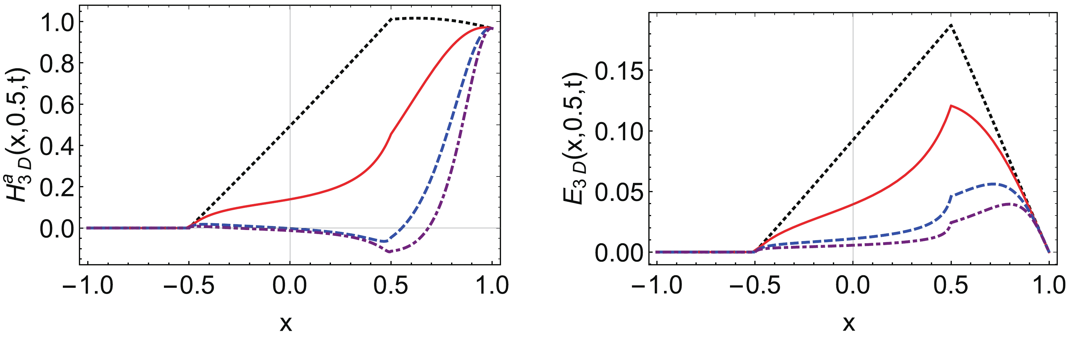
Figure 9. (color online) Pion GPDs (left panel: vector GPD, right panel: tensor GPD) at
$ \xi=0.5 $ with different t using 3D regularization: black dotted line –$ t=0 $ GeV2, red line –$ t=-1 $ GeV2, blue dashed line –$ t=-5 $ GeV2, purple dotdashed line –$ t=-10 $ GeV2.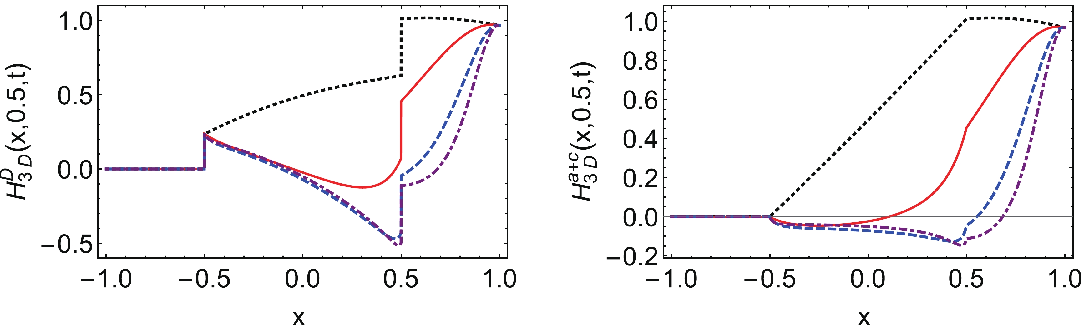
Figure 10. (color online) Pion GPDs (left panel:
$ H_{\rm{3D}}^D $ , right panel:$ H_{\rm{3D}}^a+H_{\rm{3D}}^c $ ) at$ \xi=0.5 $ with different t using PT regularization: black dotted line –$ t=0 $ GeV2, red line –$ t=-1 $ GeV2, blue dashed line –$ t=-5 $ GeV2, purple dotdashed line –$ t=-10 $ GeV2. -
In the forward limit
$ \begin{aligned}[b] u_{\rm{3D}}(x)=&\frac{3Z_{\pi }}{2\pi ^2}\int_0^{\Lambda_{\rm{3D}}}{\rm{d}}k \frac{ k^2}{(k^2+\sigma_1)^{3/2}} \\ &+\frac{3Z_{\pi }}{4\pi ^2} \int_0^{\Lambda_{\rm{3D}}}{\rm{d}}k \frac{ 3k^2 x(1-x) m_{\pi}^2 }{(k^2+\sigma_1)^{5/2}} , \end{aligned} $

(71) we plot the diagrams of u quark PDFs of pion with different values of
$ m_{\pi} $ in Fig. 11.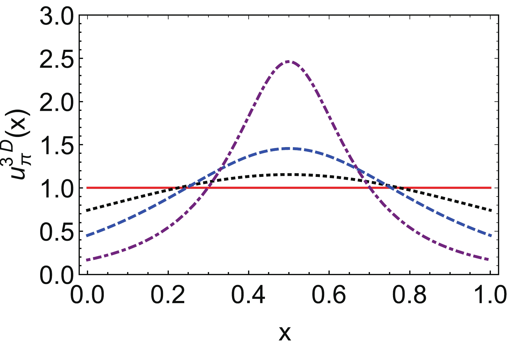
Figure 11. (color online) Pion u quark PDF with different values of
$ m_{\pi} $ using 3D regularization scheme: red line –$ m_{\pi}=0 $ GeV, black dotted line –$ m_{\pi}=0.4 $ GeV, blue dashed line –$ m_{\pi}=0.6 $ GeV, purple dotdashed line –$ m_{\pi}=0.75 $ GeV. -
$ \begin{aligned}[b] A_{1,0}^{\rm{3D}}(t)=\frac{N_cZ_{\pi } }{2\pi^2}\int_0^1 {\rm{d}}x\int_0^{\Lambda_{\rm{3D}}}{\rm{d}}k \frac{ k^2}{(k^2+\sigma_1)^{3/2}} \end{aligned} $

$ \begin{aligned}[b] \quad\quad&+\frac{N_cZ_{\pi }}{8\pi^2} \int_0^1 {\rm{d}}x \int_0^{1-x}{\rm{d}}y \int_0^{\Lambda_{\rm{3D}}}{\rm{d}}k \\ &\times \frac{3k^2(2m_{\pi }^2-(x+y)(2m_{\pi }^2-t))}{(k^2+\sigma_7)^{5/2}}, \end{aligned} $

(72) $\begin{aligned}[b] B_{1,0}^{\rm{3D}}(t)=&\frac{ N_c Z_{\pi } }{8\pi ^2} \int _0^1{\rm{d}}x \int _0^{1-x}{\rm{d}}y \int_0^{\Lambda_{\rm{3D}}}{\rm{d}}k \\&\times\frac{3k^2m_{\pi}M}{(k^2+\sigma_7)^{5/2}},\end{aligned} $

(73) $ \begin{aligned}[b] A_{2,0}^{\rm{3D}}(t)=&\frac{N_cZ_{\pi }}{4\pi ^2}\int_0^1 {\rm{d}}x\int_0^{\Lambda_{\rm{3D}}}{\rm{d}}k\frac{ k^2}{(k^2+\sigma_1)^{3/2}}\\ &+\frac{N_c Z_{\pi }}{8\pi ^2} \int_0^1 {\rm{d}}x \int_0^{1-x} {\rm{d}}y\int_0^{\Lambda_{\rm{3D}}}{\rm{d}}k (1-x-y)\\ &\times \frac{3k^2(2 m_{\pi }^2(1-x-y)+t (x+y))}{(k^2+\sigma_7)^{5/2}}, \end{aligned} $

(74) $ \begin{aligned}[b] A_{2,2}^{\rm{3D}}(t)=&-\frac{N_cZ_{\pi }}{2\pi ^2}\int_0^1 {\rm{d}}x \int_0^{\Lambda_{\rm{3D}}}{\rm{d}}k\,(1-x)\frac{ k^2}{(k^2+\sigma_1)^{3/2}}\\&-\frac{N_c Z_{\pi } }{\pi ^2} \int_0^1 {\rm{d}}x \int_0^{\Lambda_{\rm{3D}}}{\rm{d}}k\,x (1-2x) \frac{ k^2}{(k^2+\sigma_2)^{3/2}}\\ &-\frac{N_c Z_{\pi } }{2\pi^2} \int_0^1 {\rm{d}}x \int_0^{\Lambda_{\rm{3D}}}{\rm{d}}k \,\frac{ (1-x ) \left(2 m_{\pi }^2-t\right)k^2}{t(k^2+\sigma_1)^{3/2}}\\ &+\frac{N_c Z_{\pi }}{8\pi^2}\int_0^1 {\rm{d}}x \int_0^{1-x} {\rm{d}}y \int_0^{\Lambda_{\rm{3D}}}{\rm{d}}k\,\frac{3k^2\left(2 m_{\pi }^2-t\right)}{t(k^2+\sigma_7)^{5/2} }, \end{aligned} $

(75) $ \begin{aligned}[b] B_{2,0}^{\rm{3D}}(t)=&\frac{N_c Z_{\pi} }{8\pi ^2} \int_0^1 {\rm{d}}x \int_0^{1-x} {\rm{d}}y \int_0^{\Lambda_{\rm{3D}}}{\rm{d}}k \\&\times \frac{3k^2m_{\pi}M (1-x-y)}{(k^2+\sigma_7)^{5/2}}, \end{aligned} $

(76) $ A_{2,2}^{b,\rm{3D}}(t)=-\frac{N_c Z_{\pi } }{\pi ^2} \int_0^1 {\rm{d}}x \int_0^{\Lambda_{\rm{3D}}}{\rm{d}}k\, \frac{ 2M x (1-2x)k^2}{(k^2+\sigma_2)^{3/2}}. $

(77) -
In the 3D regularization scheme
$ \begin{aligned}[b] H_{\rm{3D}}\left(x,0,-{\boldsymbol{q}}_{\perp}^2\right) =&\frac{N_cZ_{\pi }}{4\pi ^2} \int_0^{\Lambda_{\rm{3D}}}{\rm{d}}k \frac{2 k^2}{(k^2+\sigma_1)^{3/2}} \\& +\frac{N_cZ_{\pi }}{8\pi ^2}\int_0^{1-x} {\rm{d}}\alpha \int_0^{\Lambda_{\rm{3D}}} {\boldsymbol{}}{\rm{d}}k \\&\times \frac{3k^2\left(2 x m_{\pi}^2+ x {\boldsymbol{q}}_{\perp}^2- {\boldsymbol{q}}_{\perp}^2\right)}{(k^2+\sigma_8)^{5/2}}, \end{aligned} $

(78) $ E_{\rm{3D}}\left(x,0,-{\boldsymbol{q}}_{\perp}^2\right)=\frac{N_cZ_{\pi }}{4\pi ^2}\int_0^{1-x} {\rm{d}}\alpha \int_0^{\Lambda_{\rm{3D}}}{\rm{d}}k \frac{3k^2m_{\pi} M }{(k^2+\sigma_8)^{5/2}}, $

(79) $ \begin{aligned}[b] u^{\rm{3D}}\left(x,{\boldsymbol{b}}_{\perp}^2\right) =&\frac{N_cZ_{\pi }}{2\pi ^2} \int \frac{{\rm{d}}^2{\boldsymbol{q}}_{\perp}}{(2 \pi )^2}\int_0^{\Lambda_{\rm{3D}}}{\rm e}^{-{\rm i}{\boldsymbol{b}}_{\perp}\cdot {\boldsymbol{q}}_{\perp}}{\rm{d}}k\frac{ k^2}{(k^2+\sigma_1)^{3/2}} \\& +\frac{N_cZ_{\pi }}{8\pi ^3}\int_0^{1-x} {\rm{d}}\alpha \int_0^{\Lambda_{\rm{3D}}}{\rm{d}}k \,{\rm e}^{ -\frac{\sqrt{{\boldsymbol{b}}_{\perp}^2(k^2+\sigma_1)} }{\sqrt{\alpha (1-\alpha -x)}} }\frac{k^2 \sqrt{{\boldsymbol{b}}_{\perp}^2} \left((1-x) \left(k^2+M^2\right)-xm_{\pi }^2 \left(2 \alpha ^2-2 \alpha +x^2+2 (\alpha -1) x+1\right)\right) }{2 \alpha ^{5/2} (1-\alpha -x)^{5/2} \left(k^2+\sigma_1\right)}\\ &-\frac{N_cZ_{\pi }}{8\pi ^3}\int_0^{1-x} {\rm{d}}\alpha \int_0^{\Lambda_{\rm{3D}}}{\rm{d}}k\,{\rm e}^{ -\frac{\sqrt{{\boldsymbol{b}}_{\perp}^2(k^2+\sigma_1)} }{\sqrt{\alpha (1-\alpha -x)}} }\frac{k^2 \left((1-x) \left(k^2+M^2\right)-x m_{\pi }^2 \left(1-\alpha ^2+\alpha +x^2-(\alpha +2) x\right)\right) }{\alpha ^2 (1-\alpha -x)^2 \left(k^2+\sigma_1\right)^{3/2}},\end{aligned} $ 
(80) $ u_{\rm{T}}^{\rm{3D}}\left(x,{\boldsymbol{b}}_{\perp}^2\right) =\frac{N_cZ_{\pi }}{8\pi^3}\int_0^{1-x} {\rm{d}}\alpha \int_0^{\Lambda_{\rm{3D}}}{\rm{d}}k\, {\rm e}^{ -\frac{\sqrt{{\boldsymbol{b}}_{\perp}^2(k^2+\sigma_1)} }{\sqrt{\alpha (1-\alpha -x)}}}\frac{k^2 m_{\pi } M \left(\sqrt{{\boldsymbol{b}}_{\perp}^2} \sqrt{k^2+\sigma_1}+\sqrt{\alpha (1-\alpha -x)}\right) }{ \alpha^{3/2} (1-\alpha -x)^{3/2} \left(k^2+\sigma_1\right)^{3/2}} , $

(81) for
$ u\left(x,{\boldsymbol{b}}_{\perp}^2\right) $ , when integrating$ {\boldsymbol{b}}_{\perp} $ one can obtain PDF$ u(x) $ in Eq. (71). We plot the diagrams of$ x *u\left(x,{\boldsymbol{b}}_{\perp}^2\right) $ and$ x *u_{\rm{T}}\left(x,{\boldsymbol{b}}_{\perp}^2\right) $ in Fig. 12.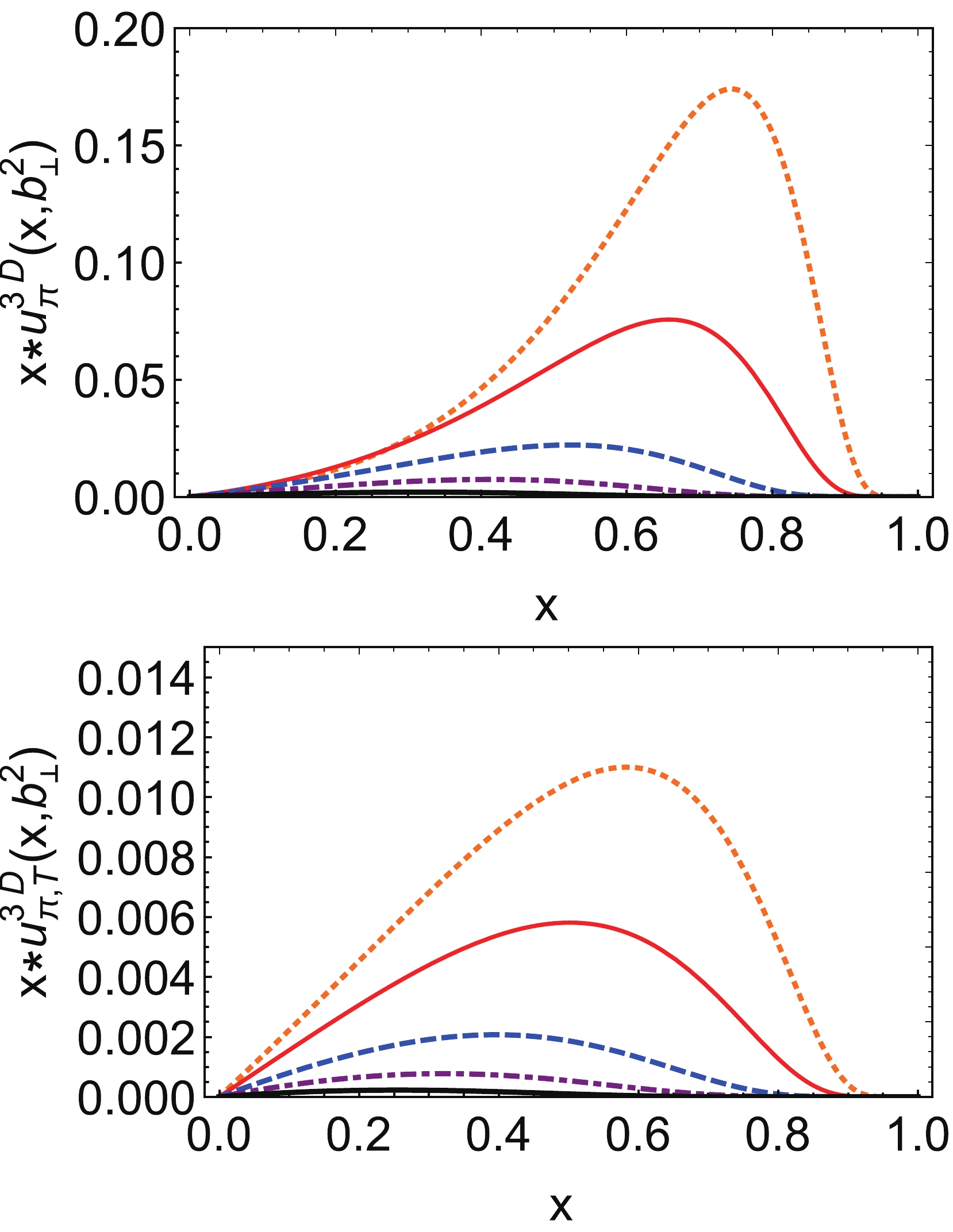
Figure 12. (color online) Impact parameter space PDFs using 3D regularization scheme: left panel –
$ x*u\left(x,{\boldsymbol{b}}_{\perp}^2\right) $ , the$ \delta^2({\boldsymbol{b}}_{\perp}) $ component first line of Eq. (80) – is suppressed in the image, and right panel –$ x*u_T\left(x,{\boldsymbol{b}}_{\perp}^2\right) $ both panels with$ {\boldsymbol{b}}_{\perp}^2=0.5 $ GeV$ ^{-2} $ – orange dotted curve,$ {\boldsymbol{b}}_{\perp}^2=1 $ GeV$ ^{-2} $ – red solid curve,$ {\boldsymbol{b}}_{\perp}^2=2.5 $ GeV$ ^{-2} $ – blue dashed curve,$ {\boldsymbol{b}}_{\perp}^2=5 $ GeV$ ^{-2} $ – purple dot-dashed curve,$ {\boldsymbol{b}}_{\perp}^2=10 $ GeV$ ^{-2} $ – thick black solid curve. -
The four-momentum cutoff in Euclidean space,
$p_E^2={\boldsymbol{p}}^2+p_4^2 < \Lambda^2$ ,$ p_0=ip_4 $ , Wick rotate the integration in gap Eq. (4), we obtained:$ \begin{aligned}[b]\\[-5pt]M=m-\frac{6 G_{\pi}}{\pi^2}\int_0^{\Lambda_{\rm{4D}}} {\rm{d}}k_E\frac{k_E^3 M}{(k_E^2+M^2)}, \end{aligned}$

(82) the pion decay constant became
$ f_{\pi}^{\rm{4D}}=\frac{N_c\sqrt{Z_{\pi }}M}{2\pi ^2}\int_0^1 {\rm{d}}x\int_0^{\Lambda_{\rm{4D}}}{\rm{d}}k\frac{k^3}{(k^2+\sigma_1)^2}, $

(83) the vector bubble diagram
$ \Pi_{\rm{VV}} $ was defined as$ \Pi_{\rm{VV}}^{\rm{4D}}(t)=-\frac{6 }{\pi ^2} \int_0^1{\rm{d}}x\int_0^{\Lambda_{\rm{4D}}} {\rm{d}}k\, \frac{x (1-x) tk^3}{(k^2+\sigma_2)^2}. $

(84) The parameters used in 4D momentum cutoff scheme are listed in Table 3.
$\Lambda _{\rm{4D}}$ 

M $G_{\pi}$ 

$G_{\rho}$ 

$G_{\omega}$ 

$m_{\pi}$ 

$f_{\pi}$ 

m $Z_{\pi}$ 

$\langle\bar{u}u\rangle$ 

0.74 0.395 9.60 7.711 6.621 0.14 0.093 0.008 17.452 −(0.216)3 Table 3. Parameter set used in 4D regularization scheme. The dressed quark mass and regularization parameters are in units of GeV, while coupling constant are in units of GeV−2.
GPDs in 4D momentum cutoff scheme
$ \begin{aligned}[b] & H_{\rm{4D}}^a\left(x,\xi,t\right)\\ =&\frac{N_cZ_{\pi }}{8\pi ^2} \left[\int_0^{\Lambda_{\rm{4D}}}{\rm{d}}k\frac{2\theta_{\bar{\xi} 1} k^3}{(k^2+\sigma_3)^2}+ \int_0^{\Lambda_{\rm{4D}}}{\rm{d}}k \frac{2\theta_{\xi 1} k^3}{(k^2+\sigma_4^2)}\right]\\ &+\frac{N_cZ_{\pi }}{8\pi ^2}\int_0^{\Lambda_{\rm{4D}}}{\rm{d}}k \frac{\theta_{\bar{\xi} \xi} }{\xi}\frac{2x k^3}{(k^2+\sigma_5)^2}\\& +\frac{N_c Z_{\pi } }{16\pi ^2}\int_0^{\Lambda_{\rm{4D}}}{\rm{d}}k\int_0^1 {\rm{d}}\alpha \frac{\theta_{\alpha \xi}}{\xi} \frac{4k^3(2 x m_{\pi}^2+(1-x)t)}{(k^2+\sigma_6)^3} ,\\[-15pt]\end{aligned} $

(85) $ E_{\rm{4D}}\left(x,\xi,t\right)=\frac{N_c Z_{\pi } }{8\pi ^2}\int_0^{\Lambda_{\rm{4D}}}{\rm{d}}k\int_0^1 {\rm{d}}\alpha \frac{\theta_{\alpha \xi}}{\xi} \frac{4k^3m_{\pi}M}{(k^2+\sigma_6)^3}, $

(86) $ H_{\rm{4D}}^b\left(x,\xi,t\right)=-\frac{N_cZ_{\pi }}{4\pi ^2} \int_0^{\Lambda_{\rm{4D}}}{\rm{d}}k \frac{\theta_{\bar{\xi} \xi} }{\xi}\frac{2Mx k^3}{(k^2+\sigma_5)^2}, $

(87) $ \begin{aligned}[b] H_{\rm{4D}}^c\left(x,\xi,t\right)=&F_{1\rho}^{\rm{4D}}(t)A_{1,0}^{\rm{4D}}(t)\frac{N_cG_{\rho }}{4\pi ^2} \int_0^{\Lambda_{\rm{4D}}}{\rm{d}}k \frac{\theta_{\bar{\xi} \xi} }{\xi}\\ &\times t\left(1-\frac{x^2}{\xi^2}\right)\frac{2k^3}{(k^2+\sigma_5)^2}, \end{aligned} $

(88) where the θ functions are defined in Eq. (50). Pion GPDs in 4D regularization scheme are plotted in Figs. 13 and 14.
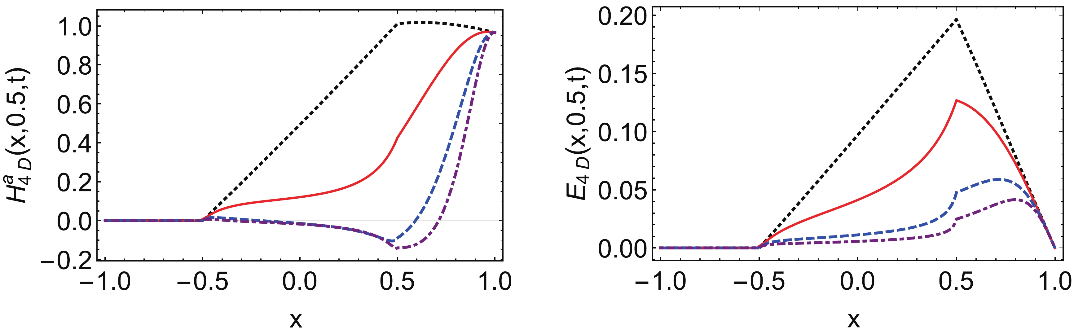
Figure 13. (color online) Pion GPDs (left panel: vector GPD, right panel: tensor GPD) at
$ \xi=0.5 $ with different t using 4D regularization: black dotted line –$ t=0 $ GeV2, red line –$ t=-1 $ GeV2, blue dashed line –$ t=-5 $ GeV2, purple dotdashed line –$ t=-10 $ GeV2.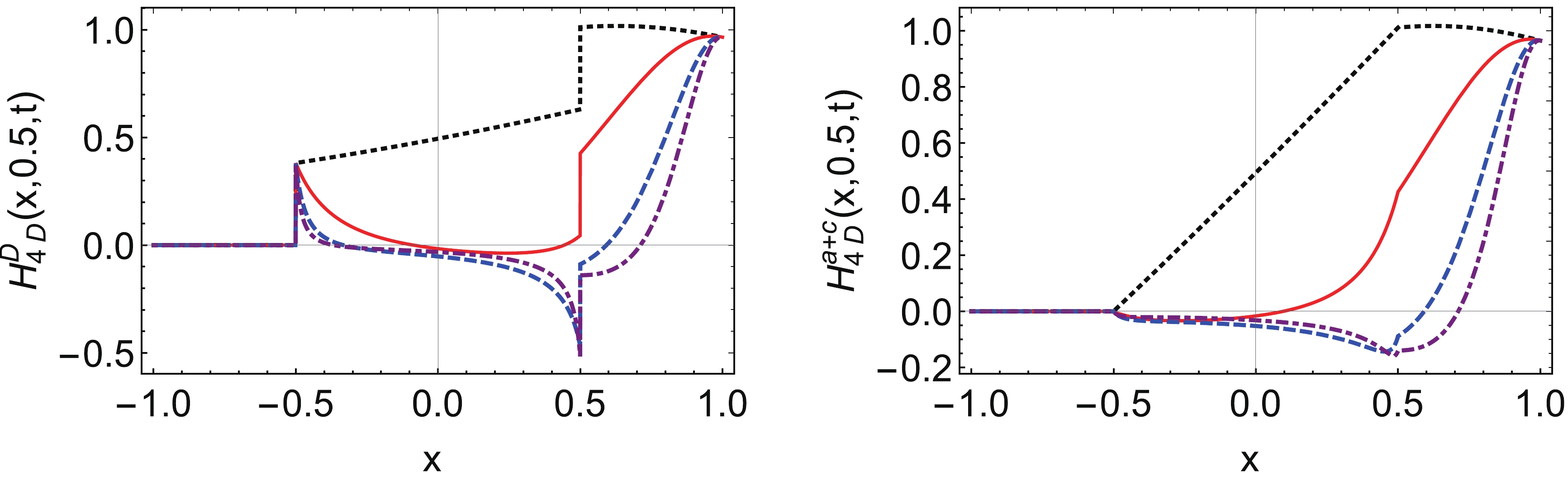
Figure 14. (color online) Pion GPDs (left panel:
$ H_{\rm{4D}}^D $ , right panel:$ H_{\rm{4D}}^a+H_{\rm{4D}}^c $ ) at$ \xi=0.5 $ with different t using PT regularization: black dotted line –$ t=0 $ GeV2, red line –$ t=-1 $ GeV2, blue dashed line –$ t=-5 $ GeV2, purple dotdashed line –$ t=-10 $ GeV2. -
In the forward limit
$ \begin{aligned}[b] u_{\rm{4D}}(x)=&\frac{3Z_{\pi }}{4\pi ^2}\int_0^{\Lambda_{\rm{4D}}}{\rm{d}}k \frac{ 2k^3}{(k^2+\sigma_1)^2} \\ &+\frac{3Z_{\pi }}{4\pi ^2} \int_0^{\Lambda_{\rm{4D}}}{\rm{d}}k \frac{ 4k^3 x(1-x) m_{\pi}^2 }{(k^2+\sigma_1)^3} , \end{aligned} $

(89) we have plot the PDF in 4D regularization scheme in Fig. 15.
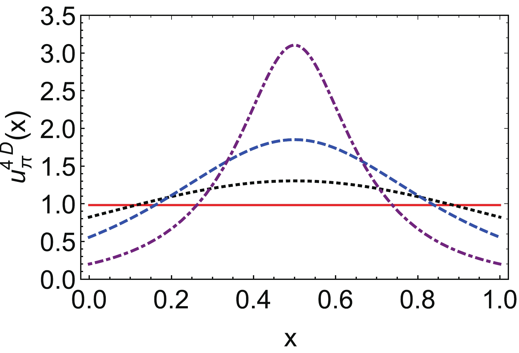
Figure 15. (color online) Pion u quark PDF with different values of
$ m_{\pi} $ using 4D regularization scheme: red line –$ m_{\pi}=0 $ GeV, black dotted line –$ m_{\pi}=0.4 $ GeV, blue dashed line –$ m_{\pi}=0.6 $ GeV, purple dotdashed line –$ m_{\pi}=0.75 $ GeV. -
$ \begin{aligned}[b] A_{1,0}^{\rm{4D}}(t)=&\frac{N_cZ_{\pi } }{4\pi^2}\int_0^1 {\rm{d}}x\int_0^{\Lambda_{\rm{4D}}}{\rm{d}}k \frac{ 2k^3}{(k^2+\sigma_1)^2}+\frac{N_cZ_{\pi }}{8\pi^2} \int_0^1 {\rm{d}}x \\ &\times \int_0^{1-x} {\rm{d}}y \int_0^{\Lambda_{\rm{4D}}}{\rm{d}}k \frac{4k^3(2m_{\pi }^2-(x+y)(2m_{\pi }^2-t))}{(k^2+\sigma_7)^3},\end{aligned} $

(90) $ B_{1,0}^{\rm{4D}}(t)=\frac{ N_c Z_{\pi } }{8\pi ^2} \int _0^1{\rm{d}}x \int _0^{1-x}{\rm{d}}y \int_0^{\Lambda_{\rm{4D}}}{\rm{d}}k\frac{4k^3m_{\pi}M}{(k^2+\sigma_7)^3}, $

(91) $ \begin{aligned}[b] A_{2,0}^{\rm{4D}}(t)=&\frac{N_cZ_{\pi }}{8\pi ^2}\int_0^1 {\rm{d}}x\int_0^{\Lambda_{\rm{4D}}}{\rm{d}}k\frac{ 2k^3}{(k^2+\sigma_1)^2}\\&+\frac{N_c Z_{\pi }}{8\pi ^2} \int_0^1 {\rm{d}}x \int_0^{1-x} {\rm{d}}y\int_0^{\Lambda_{\rm{4D}}}{\rm{d}}k (1-x-y)\\ &\times \frac{4k^3(2 m_{\pi }^2(1-x-y)+t (x+y))}{(k^2+\sigma_7)^3}, \end{aligned} $

(92) $ \begin{aligned}[b] A_{2,2}^{\rm{4D}}(t)=&-\frac{N_cZ_{\pi }}{4\pi ^2}\int_0^1 {\rm{d}}x \int_0^{\Lambda_{\rm{4D}}}{\rm{d}}k\,(1-x)\frac{ 2k^3}{(k^2+\sigma_1)^2}\\&-\frac{N_c Z_{\pi } }{2\pi ^2} \int_0^1 {\rm{d}}x \int_0^{\Lambda_{\rm{4D}}}{\rm{d}}k\,x (1-2x) \frac{ 2k^3}{(k^2+\sigma_2)^2}\\ &-\frac{N_c Z_{\pi } }{4\pi^2} \int_0^1 {\rm{d}}x \int_0^{\Lambda_{\rm{4D}}}{\rm{d}}k \,\frac{ (1-x ) \left(2 m_{\pi }^2-t\right)2k^3}{t(k^2+\sigma_1)^2}\\ &+\frac{N_c Z_{\pi }}{8\pi^2}\int_0^1 {\rm{d}}x \int_0^{1-x} {\rm{d}}y \int_0^{\Lambda_{\rm{4D}}}{\rm{d}}k\,\frac{4k^3\left(2 m_{\pi }^2-t\right)}{t(k^2+\sigma_7)^3},\\[-15pt] \end{aligned} $

(93) $ \begin{aligned}[b] B_{2,0}^{\rm{4D}}(t)=&\frac{N_c Z_{\pi} }{8\pi ^2} \int_0^1 {\rm{d}}x \int_0^{1-x} {\rm{d}}y \int_0^{\Lambda_{\rm{4D}}}{\rm{d}}k \\ &\times \frac{4k^3m_{\pi}M (1-x-y)}{(k^2+\sigma_7)^3}, \end{aligned} $

(94) $ A_{2,2}^{b,\rm{4D}}(t)=-\frac{N_c Z_{\pi } }{\pi ^2} \int_0^1 {\rm{d}}x \int_0^{\Lambda_{\rm{4D}}}{\rm{d}}k\, \frac{ 2M x (1-2x)k^3}{(k^2+\sigma_2)^2}. $

(95) -
$ \begin{aligned}[b] H_{\rm{4D}}\left(x,0,-{\boldsymbol{q}}_{\perp}^2\right)=\frac{N_cZ_{\pi }}{4\pi ^2} \int_0^{\Lambda_{\rm{4D}}}{\rm{d}}k \frac{2 k^3}{(k^2+\sigma_1)^2} \end{aligned} $

$ \begin{aligned}[b] \quad\quad& +\frac{N_cZ_{\pi }}{8\pi ^2}\int_0^{1-x} {\rm{d}}\alpha \int_0^{\Lambda_{\rm{4D}}} {\rm{d}}k \\&\times \frac{4k^3\left(2 x m_{\pi}^2+ x {\boldsymbol{q}}_{\perp}^2- {\boldsymbol{q}}_{\perp}^2\right)}{(k^2+\sigma_8)^3}, \end{aligned} $

(96) $ E_{\rm{4D}}\left(x,0,-{\boldsymbol{q}}_{\perp}^2\right)=\frac{N_cZ_{\pi }}{4\pi ^2}\int_0^{1-x} {\rm{d}}\alpha \int_0^{\Lambda_{\rm{4D}}}{\rm{d}}k \frac{4k^3m_{\pi} M }{(k^2+\sigma_8)^3}, $

(97) $ \begin{aligned}[b] u^{\rm{4D}}\left(x,{\boldsymbol{b}}_{\perp}^2\right)=&\frac{N_cZ_{\pi }}{4\pi ^2} \int \frac{{\rm{d}}^2{\boldsymbol{q}}_{\perp}}{(2 \pi )^2}\int_0^{\Lambda_{\rm{4D}}}{\rm e}^{-{\rm i}{\boldsymbol{b}}_{\perp}\cdot {\boldsymbol{q}}_{\perp}}{\rm{d}}k\frac{ k^2}{(k^2+\sigma_1)^{3/2}} \\& +\frac{N_cZ_{\pi }}{16\pi ^3}\int_0^{1-x} {\rm{d}}\alpha \int_0^{\Lambda_{\rm{4D}}}{\rm{d}}k\, {{K}}_1\left[\frac{\sqrt{{\boldsymbol{b}}_{\perp}^2} \sqrt{k^2+\sigma_1}}{\sqrt{\alpha (1-x-\alpha )}}\right] \frac{2 k^3 (x-1) \sqrt{{\boldsymbol{b}}_{\perp}^2} }{ \alpha ^{5/2} (1-\alpha -x)^{5/2} \sqrt{k^2+\sigma_1}}\\& +\frac{N_cZ_{\pi }}{16\pi ^3}\int_0^{1-x} {\rm{d}}\alpha \int_0^{\Lambda_{\rm{4D}}}{\rm{d}}k\, {\boldsymbol{b}}_{\perp}^2 k^3 \, {{K}}_2\left[\frac{\sqrt{{\boldsymbol{b}}_{\perp}^2} \sqrt{k^2+\sigma_1}}{\sqrt{\alpha (1-x-\alpha)}}\right]\frac{\left((1-x) \left(k^2+M^2\right)-xm_{\pi }^2 \left(2 \alpha ^2-2 \alpha +x^2+2 (\alpha -1) x+1\right)\right) }{2 \alpha ^3 (1-\alpha -x)^3 \left(k^2+\sigma_1\right)}, \end{aligned} $

(98) $ u_{\rm{T}}^{\rm{4D}}\left(x,{\boldsymbol{b}}_{\perp}^2\right)=\frac{N_cZ_{\pi }}{16\pi^3}\int_0^{1-x} {\rm{d}}\alpha \int_0^{\Lambda_{\rm{4D}}}{\rm{d}}k \frac{k^3 m_{\pi } M {\boldsymbol{b}}_{\perp}^2 }{ \alpha ^2 (1-\alpha-x)^2 \left(k^2+\sigma_1\right)}{K}_2\left[\frac{\sqrt{{\boldsymbol{b}}_{\perp}^2} \sqrt{k^2+\sigma_1}}{\sqrt{\alpha (1-x-\alpha )}}\right], $

(99) where
${K}_1$ and${K}_2$ are the Bessel function of the second kind${K}_n(z)$ , for$ u^{\rm{4D}}\left(x,{\boldsymbol{b}}_{\perp}^2\right) $ , when integrating$ {\boldsymbol{b}}_{\perp} $ we obtained PDF$ u(x) $ in Eq. (89). We plot the diagrams of$ x *u^{\rm{4D}}\left(x,{\boldsymbol{b}}_{\perp}^2\right) $ and$ x *u_{\rm{T}}^{\rm{4D}}\left(x,{\boldsymbol{b}}_{\perp}^2\right) $ in Fig. 16.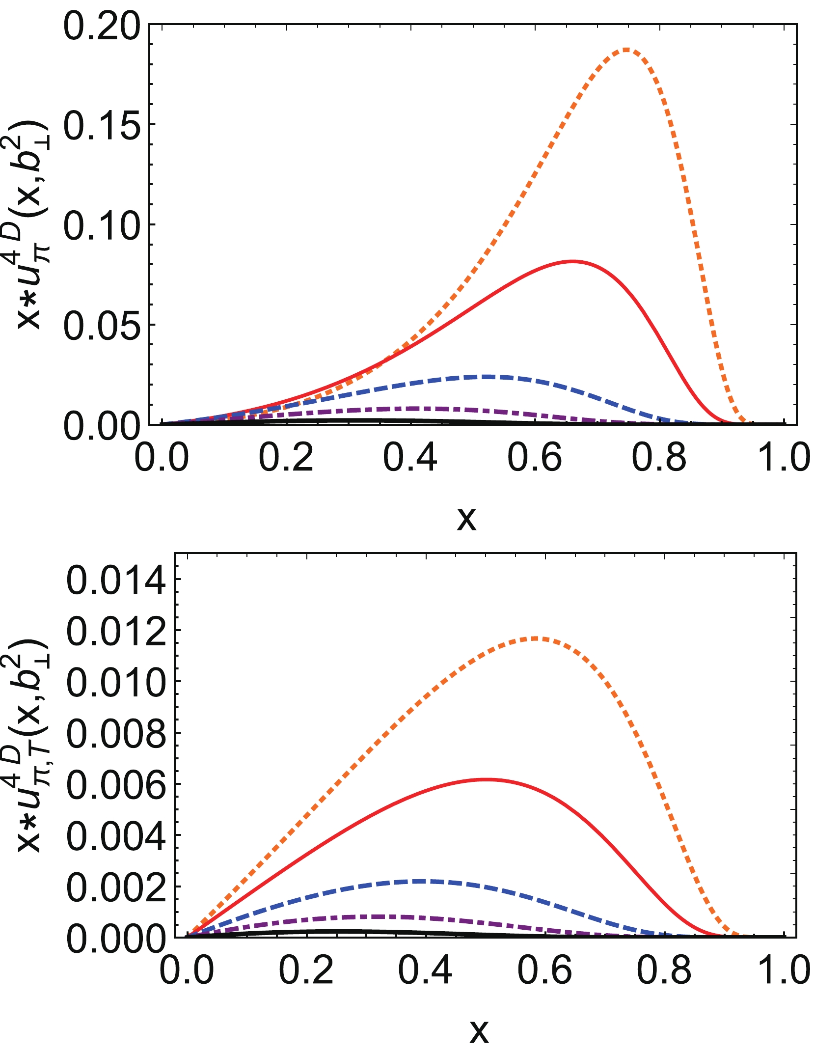
Figure 16. (color online) Impact parameter space PDFs using 4D regularization scheme: left panel –
$ x*u\left(x,{\boldsymbol{b}}_{\perp}^2\right) $ , the$ \delta^2({\boldsymbol{b}}_{\perp}) $ component first line of Eq. (98) – is suppressed in the image, and right panel –$ x*u_T\left(x,{\boldsymbol{b}}_{\perp}^2\right) $ both panels with$ {\boldsymbol{b}}_{\perp}^2=0.5 $ GeV-2 – orange dotted curve,$ {\boldsymbol{b}}_{\perp}^2=1 $ GeV-2 – red solid curve,$ {\boldsymbol{b}}_{\perp}^2=2.5 $ GeV-2 – blue dashed curve,$ {\boldsymbol{b}}_{\perp}^2=5 $ GeV-2 – purple dot-dashed curve,$ {\boldsymbol{b}}_{\perp}^2=10 $ GeV-2 – thick black solid curve. -
he PV scheme has an attractive feature, which is it keeps the gauge invariance. In PV regularization, to get rid of the divergences from loop integrals, people introduced the virtually heavy particles [49]
$ \frac{1}{k^2-M^2}\rightarrow \sum\limits_i c_i \frac{1}{k^2-M_i^2}, $

(100) where the labels run from
$ i=0 $ to$ i=2 $ $ M_i^2=M^2+\alpha_i\Lambda_i^2, $

(101) where
$ \begin{aligned}[b] & c_0=1,\quad c_1=1,\quad c_2=-2;\\ & \alpha_0=0,\quad\alpha_1=2,\quad\alpha_2=1; \end{aligned} $

(102) then the gap equation became
$ M =m-\frac{3G_{\pi}M}{\pi^2}\sum\limits_ic_iM_i^2\log\left[M_i^2/M^2\right], $

(103) the pion decay constant became
$ f_{\pi}^{\rm{PV}}=\frac{N_c\sqrt{Z_{\pi }}M}{4\pi ^2}\int_0^1 {\rm{d}}x \log \left[\frac{\left(\Lambda_{\rm{PV}}^2+\sigma_1\right)^2}{\sigma_1 \left(2 \Lambda_{\rm{PV}}^2+\sigma_1\right)}\right], $

(104) the bubble diagram
$ \Pi_{\rm{VV}} $ is$ \Pi_{\rm{VV}}^{\rm{PV}}(t)=-\frac{3 }{\pi ^2} \int_0^1{\rm{d}}x\, x (1-x) t\log \left[\frac{\left(\Lambda_{\rm{PV}}^2+\sigma_2\right)^2}{\sigma_2\left(2 \Lambda_{\rm{PV}}^2+\sigma_2\right)}\right]. $

(105) The parameters used in PV regularization scheme are listed in Table 4.
$\Lambda _{\rm{PV}}$ 

M $G_{\pi}$ 

$G_{\rho}$ 

$G_{\omega}$ 

$m_{\pi}$ 

$f_{\pi}$ 

m $Z_{\pi}$ 

$\langle\bar{u}u\rangle$ 

0.63 0.4 9.724 8.407 7.451 0.14 0.093 0.008 18.17 −(0.216)3 Table 4. Parameter set used in PV regularization scheme. The dressed quark mass and regularization parameters are in units of GeV, while coupling constant are in units of GeV−2.
Then, we obtained the pion GPDs in PV scheme
$ \begin{aligned}[b] H_{\rm{PV}}^a\left(x,\xi,t\right) =& \frac{N_cZ_{\pi }}{8\pi ^2}\theta_{\bar{\xi} 1} \log \left[\frac{\left(\Lambda_{\rm{PV}}^2+\sigma_3\right)^2}{\sigma_3 \left(2 \Lambda_{\rm{PV}}^2+\sigma_3\right)}\right]\\& + \frac{N_cZ_{\pi }}{8\pi ^2}\theta_{\bar{\xi} 1} \log \left[\frac{\left(\Lambda_{\rm{PV}}^2+\sigma_4\right)^2}{\sigma_4 \left(2 \Lambda_{\rm{PV}}^2+\sigma_4\right)}\right]\\& +\frac{N_cZ_{\pi }}{8\pi ^2}\frac{\theta_{\bar{\xi} \xi} }{\xi} x\log \left[\frac{\left(\Lambda_{\rm{PV}}^2+\sigma_5\right)^2}{\sigma_5 \left(2 \Lambda_{\rm{PV}}^2+\sigma_5\right)}\right]\\& +\frac{N_c Z_{\pi } }{16\pi ^2}\int_0^1 {\rm{d}}\alpha \frac{\theta_{\alpha \xi}}{\xi} (2 x m_{\pi}^2+(1-x)t)\\ &\times \left(\frac{1}{\sigma_6+2\Lambda_{\rm{PV}}^2}-\frac{2}{\sigma_6+\Lambda_{\rm{PV}}^2}-\frac{1}{\sigma_6} \right) , \end{aligned} $

(106) $ \begin{aligned}[b] E_{\rm{PV}}\left(x,\xi,t\right)=&\frac{N_c Z_{\pi } }{8\pi ^2}\int_0^1 {\rm{d}}\alpha \frac{\theta_{\alpha \xi}}{\xi} m_{\pi}M\\ &\times \left(\frac{1}{\sigma_6+2\Lambda_{\rm{PV}}^2}-\frac{2}{\sigma_6+\Lambda_{\rm{PV}}^2}-\frac{1}{\sigma_6} \right), \end{aligned} $

(107) $ H_{\rm{PV}}^b\left(x,\xi,t\right)=-\frac{N_cZ_{\pi }}{4\pi ^2} \frac{\theta_{\bar{\xi} \xi} }{\xi} Mx \log \left[\frac{\left(\Lambda_{\rm{PV}}^2+\sigma_5\right)^2}{\sigma_5 \left(2 \Lambda_{\rm{PV}}^2+\sigma_5\right)}\right], $

(108) $ \begin{aligned}[b] H_{\rm{PV}}^c\left(x,\xi,t\right)=&F_{1\rho}^{\rm{PV}}(t)A_{1,0}^{\rm{PV}}(t)\frac{N_cG_{\rho }}{4\pi ^2} \frac{\theta_{\bar{\xi} \xi} }{\xi}t\left(1-\frac{x^2}{\xi^2}\right)\\&\times \log \left[\frac{\left(\Lambda_{\rm{PV}}^2+\sigma_5\right)^2}{\sigma_5 \left(2 \Lambda_{\rm{PV}}^2+\sigma_5\right)}\right], \end{aligned} $

(109) The pion GPDs in PV regularization scheme are plotted in Figs. 17 and 18.

Figure 17. (color online) Pion GPDs (left panel: vector GPD, right panel: tensor GPD) at
$ \xi=0.5 $ with different t using PV regularization: black dotted line –$ t=0 $ GeV2, red line –$ t=-1 $ GeV2, blue dashed line –$ t=-5 $ GeV2, purple dotdashed line –$ t=-10 $ GeV2.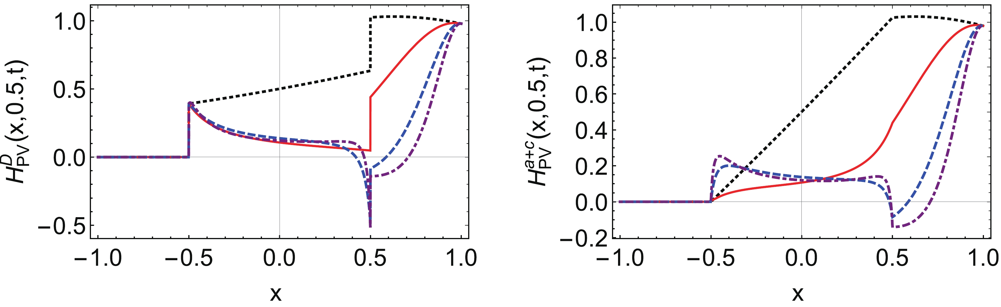
Figure 18. (color online) Pion GPDs (left panel:
$ H_{\rm{PV}}^D $ , right panel:$ H_{\rm{PV}}^a+H_{\rm{PV}}^c $ ) at$ \xi=0.5 $ with different t using PT regularization: black dotted line –$ t=0 $ GeV2, red line –$ t=-1 $ GeV2, blue dashed line –$ t=-5 $ GeV2, purple dotdashed line –$ t=-10 $ GeV2. -
In the forward limit
$ \begin{aligned}[b] u_{\rm{PV}}(x)=&\frac{3Z_{\pi }}{4\pi ^2} \log \left[\frac{\left(\Lambda_{\rm{PV}} ^2+\sigma_1\right)^2}{\sigma_1\left(2 \Lambda_{\rm{PV}} ^2+\sigma_1\right)}\right]\\& + \frac{3Z_{\pi }}{4\pi ^2} x(1-x) m_{\pi}^2 \left(\frac{1}{\sigma_1+2\Lambda_{\rm{PV}}^2}-\frac{2}{\sigma_1+\Lambda_{\rm{PV}}^2}+\frac{1}{\sigma_1} \right) , \end{aligned} $

(110) we plot the PDF in PV regularization scheme in Fig. 19. From Figs. 7, 11, 15 and 19 we saw that in PT and PV regularization schemes, pion PDFs were softer, in the 3D and 4D regularization schemes the peaks were sharper, that's because the value of constituent quark mass M. There is a factor
$ \sigma_1=(M^2-x(1-x)m_{\pi}^2) $ in all the PDFs, when M is not large enough but$ m_{\pi} $ became too large, this term would be negative, then the result would not be right, we choose$ M\approx 0.4 $ GeV, the maximum value of pion mass was$ m_{\pi}=0.75 $ GeV. When the value of$ \sigma_1 $ was nearer to zero, the maximum value of PDF would be larger, then the peak would be sharper. The values of M in 3D and 4D regularization schemes were smaller, so the peaks were sharper. For$ m_{\pi}=0.14 $ GeV, the values of PDFs in all the regularization schemes was almost one.
Figure 19. (color online) Pion u quark PDF with different values of
$ m_{\pi} $ using PV regularization: red line –$ m_{\pi}=0 $ GeV, black dotted line –$ m_{\pi}=0.4 $ GeV, blue dashed line –$ m_{\pi}=0.6 $ GeV, purple dotdashed line –$ m_{\pi}=0.75 $ GeV. -
$ \begin{aligned}[b] A_{1,0}^{\rm{PV}}(t)=&\frac{N_cZ_{\pi } }{4\pi^2}\int_0^1 {\rm{d}}x\log \left[\frac{\left(\Lambda_{\rm{PV}} ^2+\sigma_1\right)^2}{\sigma_1\left(2 \Lambda_{\rm{PV}} ^2+\sigma_1\right)}\right]\\ &+\frac{N_cZ_{\pi }}{8\pi^2} \int_0^1 {\rm{d}}x \int_0^{1-x}{\rm{d}}y\, (2m_{\pi }^2-(x+y)(2m_{\pi }^2-t))\\ &\times \left(\frac{1}{\sigma_7+2\Lambda_{\rm{PV}}^2}-\frac{2}{\sigma_7+\Lambda_{\rm{PV}}^2}+\frac{1}{\sigma_7} \right), \end{aligned} $

(111) $ \begin{aligned}[b] B_{1,0}^{\rm{PV}}(t)=&\frac{ N_c Z_{\pi } }{8\pi ^2} \int _0^1{\rm{d}}x \int _0^{1-x}{\rm{d}}y \,m_{\pi}M\\ &\times \left(\frac{1}{\sigma_7+2\Lambda_{\rm{PV}}^2}-\frac{2}{\sigma_7+\Lambda_{\rm{PV}}^2}+\frac{1}{\sigma_7} \right), \end{aligned} $

(112) $ \begin{aligned}[b] A_{2,0}^{\rm{PV}}(t)=&\frac{N_cZ_{\pi }}{8\pi ^2}\int_0^1 {\rm{d}}x \log \left[\frac{\left(\Lambda_{\rm{PV}} ^2+\sigma_1\right)^2}{\sigma_1\left(2 \Lambda_{\rm{PV}} ^2+\sigma_1\right)}\right]\\ &+\frac{N_c Z_{\pi }}{8\pi ^2} \int_0^1 {\rm{d}}x \int_0^{1-x} {\rm{d}}y \,(1-x-y)\\ &\times (2 m_{\pi }^2(1-x-y)+t (x+y))\\ &\times \left(\frac{1}{\sigma_7+2\Lambda_{\rm{PV}}^2}-\frac{2}{\sigma_7+\Lambda_{\rm{PV}}^2}+\frac{1}{\sigma_7} \right), \end{aligned} $

(113) $ \begin{aligned}[b] A_{2,2}^{\rm{PV}}(t)=&-\frac{N_cZ_{\pi }}{4\pi ^2}\int_0^1 {\rm{d}}x \,(1-x)\log \left[\frac{\left(\Lambda_{\rm{PV}} ^2+\sigma_1\right)^2}{\sigma_1\left(2 \Lambda_{\rm{PV}} ^2+\sigma_1\right)}\right]\\ &-\frac{N_c Z_{\pi } }{2\pi ^2} \int_0^1 {\rm{d}}x \,x (1-2x) \log \left[\frac{\left(\Lambda_{\rm{PV}} ^2+\sigma_2\right)^2}{\sigma_2\left(2 \Lambda_{\rm{PV}} ^2+\sigma_2\right)}\right]\\&-\frac{N_c Z_{\pi } }{4\pi^2} \int_0^1 {\rm{d}}x \,\frac{ (1-x ) \left(2 m_{\pi }^2-t\right)}{t}\\ &\times \log \left[\frac{\left(\Lambda_{\rm{PV}} ^2+\sigma_1\right)^2}{\sigma_1\left(2 \Lambda_{\rm{PV}} ^2+\sigma_1\right)}\right]\\ &+\frac{N_c Z_{\pi }}{8\pi^2}\int_0^1 {\rm{d}}x \int_0^{1-x} {\rm{d}}y \,\frac{\left(2 m_{\pi }^2-t\right)}{t}\\ &\times \left(\frac{1}{\sigma_7+2\Lambda_{\rm{PV}}^2}-\frac{2}{\sigma_7+\Lambda_{\rm{PV}}^2}+\frac{1}{\sigma_7} \right), \end{aligned} $

(114) $ \begin{aligned}[b] B_{2,0}^{\rm{PV}}(t)=&\frac{N_c Z_{\pi} }{8\pi ^2} \int_0^1 {\rm{d}}x \int_0^{1-x} {\rm{d}}y \,m_{\pi}M (1-x-y)\\ &\times \left(\frac{1}{\sigma_7+2\Lambda_{\rm{PV}}^2}-\frac{2}{\sigma_7+\Lambda_{\rm{PV}}^2}+\frac{1}{\sigma_7} \right), \end{aligned} $

(115) $ \begin{aligned}[b] A_{2,2}^{b,\rm{PV}}(t)=&-\frac{N_c Z_{\pi } }{\pi ^2} \int_0^1 {\rm{d}}x \,M x (1-2x)\\ &\times\log \left[\frac{\left(\Lambda_{\rm{PV}} ^2+\sigma_2\right)^2}{\sigma_2\left(2 \Lambda_{\rm{PV}} ^2+\sigma_2\right)}\right]. \end{aligned} $

(116) We have listed charge radius and the values of GFFs at
$ t=0 $ in Table 5. The bare charge radius in PT regularization is the biggest, in the 3D momentum cutoff is the smallest, but do not have too much difference. For the dressed pion charge radius, the value in PT regularization is larger and approximates the experiment data$ r_{\pi}=0.66 $ fm. The values of the quark mass distribution$ A_{2,0}(0) $ and the quark pressure distribution$ A_{2,2}^D(0) $ , in the PV regularization are the largest, but for the anomalous magnetic moment$ B_{1,0}(0) $ and$ B_{2,0}(0) $ in the PT regularization do not have too much difference with the results in PV regularization. The low-energy theorem requires$ \theta_1(0)-\theta_2(0)={\cal{O}}(m_{\pi}^2) $ , if we do not consider the contribution of the contact term, we saw from Table 5 that$ A_{2,0}(0) $ and$ |A_{2,2}(0)| $ is different. When considering the contact contribution term, the value of$ |A_{2,2}^D(0)| $ is close to$ A_{2,0}(0) $ .$r_{\pi}$ 

$r_{\pi}^D$ 

$A_{2,0}(0)$ 

$A_{2,2}(0)$ 

$A_{2,2}^D(0)$ 

$B_{1,0}(0)$ 

$B_{2,0}(0)$ 

PT 0.457 0.628 0.500 −0.161 −0.418 0.150 0.050 3D 0.444 0.578 0.500 −0.161 −0.415 0.140 0.047 4D 0.455 0.583 0.500 −0.161 −0.415 0.147 0.049 PV 0.454 0.590 0.507 −0.163 −0.424 0.148 0.050 Table 5. Charge radius and GFFs at t = 0, charge radius are in units of fm.
In Figs. 20 – 22 we plot the diagrams of FFs. Fig. 20 shows the electromagnetic FFs, the bare FF in the left panel and the dressed FF in the right panel. Fig. 21 plots the quark mass distribution
$ A_{2,0}(t) $ in the left panel and the quark pressure distribution$ A_{2,2}^D(t) $ in the right panel, the gravitational FFs in PT regularization are the softest. Fig. 22 gives the tensor FFs$ B_{1,0}(t) $ and$ B_{2,0}(t) $ , the tensor FFs are almost the same slope in different regularization schemes, the four lines are almost parallel, but the values in PT regularization are the largest.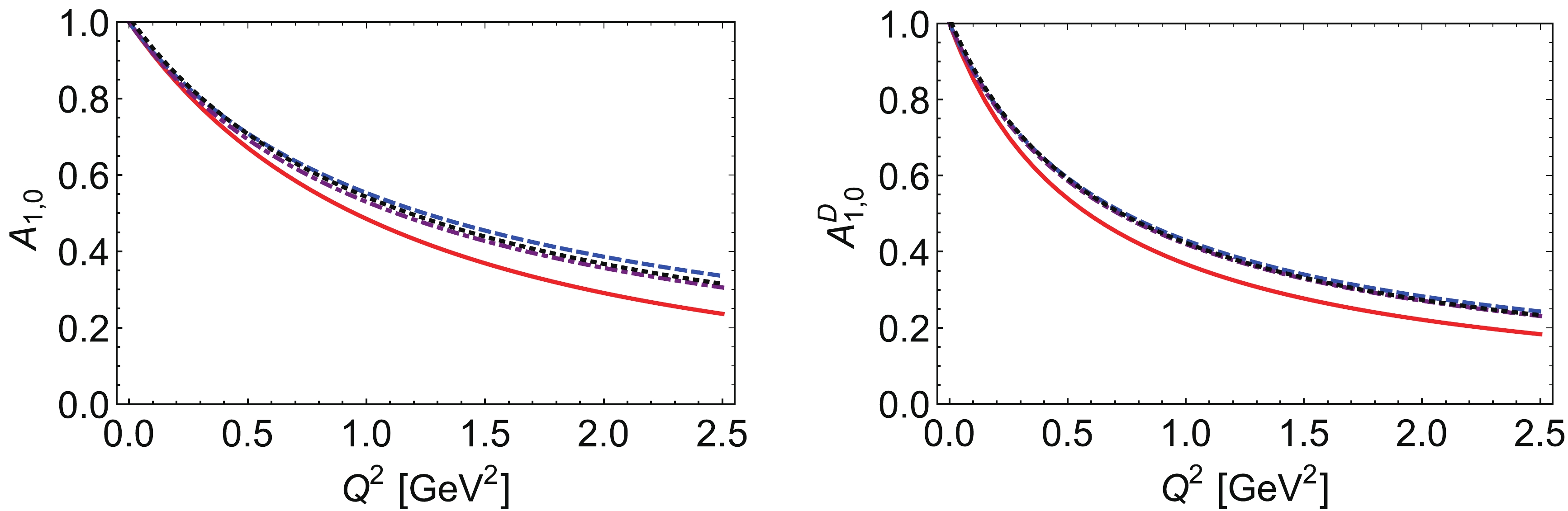
Figure 20. (color online) Pion electromagnetic FFs (left panel: bare FF, right panel: dressed FF) using different regularization schemes: red line – PT regularization, blue dashed line – 3D regularization, purple dotdashed line – 4D regularization, black dotted line – PV regularization.
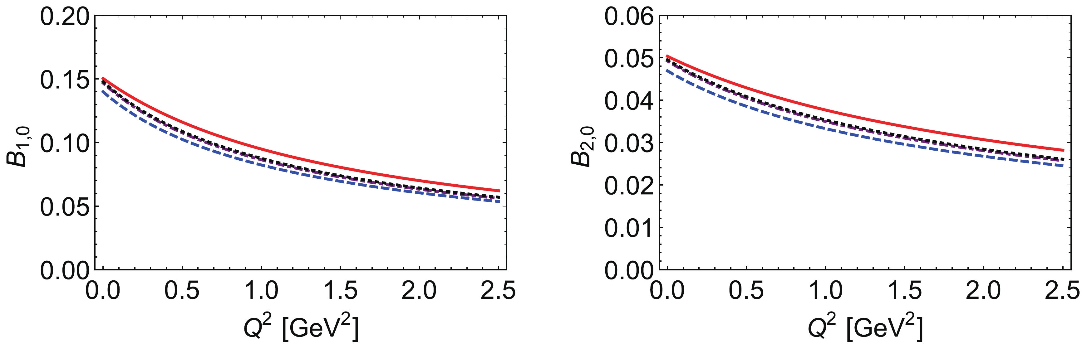
Figure 22. (color online) Pion tensor FFs (left panel:
$ B_{1,0}(t) $ , right panel:$ B_{2,0}(t) $ ) using different regularization schemes: red line – PT regularization, blue dashed line – 3D regularization, purple dotdashed line – 4D regularization, black dotted line – PV regularization.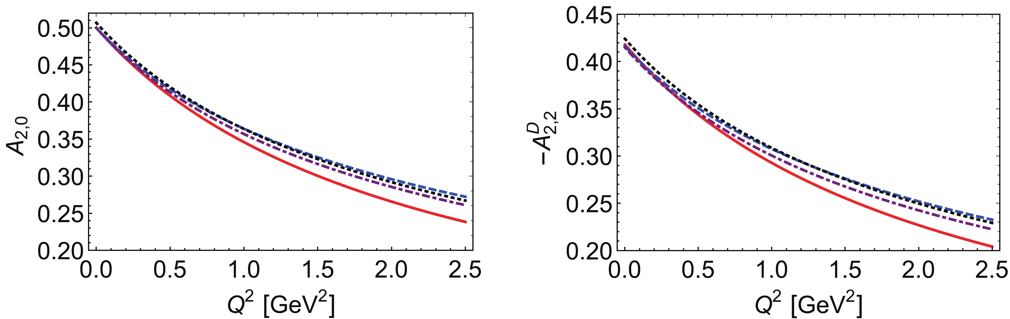
Figure 21. (color online) Pion generalized vector FFs (left panel:
$ A_{2,0}(t) $ , right panel:$ A_{2,2}^D(t) $ ) using different regularization schemes: red line – PT regularization, blue dashed line – 3D regularization, purple dotdashed line – 4D regularization, black dotted line – PV regularization. -
$ \begin{aligned}[b] H_{\rm{PV}}\left(x,0,-{\boldsymbol{q}}_{\perp}^2\right) =&\frac{N_cZ_{\pi }}{4\pi ^2} \log \left[\frac{\left(\Lambda_{\rm{PV}} ^2+\sigma_1\right)^2}{\sigma_1\left(2 \Lambda_{\rm{PV}} ^2+\sigma_1\right)}\right] \\& +\frac{N_cZ_{\pi }}{8\pi ^2}\int_0^{1-x} {\rm{d}}\alpha \left(2 x m_{\pi}^2+ x {\boldsymbol{q}}_{\perp}^2- {\boldsymbol{q}}_{\perp}^2\right)\\& \times \left(\frac{1}{\sigma_8+2\Lambda_{\rm{PV}}^2}-\frac{2}{\sigma_8+\Lambda_{\rm{PV}}^2}+\frac{1}{\sigma_8} \right), \end{aligned} $

(117) $ \begin{aligned}[b] E_{\rm{PV}}\left(x,0,-{\boldsymbol{q}}_{\perp}^2\right)=&\frac{N_cZ_{\pi }}{4\pi ^2}\int_0^{1-x} {\rm{d}}\alpha\,m_{\pi} M \\ &\times \left(\frac{1}{\sigma_8+2\Lambda_{\rm{PV}}^2}-\frac{2}{\sigma_8+\Lambda_{\rm{PV}}^2}+\frac{1}{\sigma_8} \right), \end{aligned} $

(118) $ \begin{aligned}[b] u^{\rm{PV}}\left(x,{\boldsymbol{b}}_{\perp}^2\right) =&\frac{N_cZ_{\pi }}{4\pi ^2} \int \frac{{\rm{d}}^2{\boldsymbol{q}}_{\perp}}{(2 \pi )^2} {\rm e}^{-{\rm i}{\boldsymbol{b}}_{\perp}\cdot {\boldsymbol{q}}_{\perp}}\log \left[\frac{\left(\Lambda_{\rm{PV}}^2+\sigma_1\right)^2}{\sigma_1 \left(2 \Lambda_{\rm{PV}}^2+\sigma_1\right)}\right] \\& +\frac{N_cZ_{\pi }}{16\pi ^3}\int_0^{1-x} {\rm{d}}\alpha \, {\rm{K}}_0\left[\frac{\sqrt{{\boldsymbol{b}}_{\perp}^2(2 \Lambda_{\rm{PV}}^2+\sigma_1)} }{\sqrt{\alpha (1-x-\alpha )}}\right] \frac{\left((1-x) \left(2\Lambda_{\rm{PV}}^2+M^2\right)-m_{\pi }^2 x \left(2 \alpha ^2-2 \alpha +x^2+2 (\alpha -1) x+1\right)\right) }{\alpha ^2 (\alpha +x-1)^2} \\& -\frac{N_cZ_{\pi }}{8\pi ^3}\int_0^{1-x} {\rm{d}}\alpha \, {K}_0\left[\frac{\sqrt{{\boldsymbol{b}}_{\perp}^2(\Lambda_{\rm{PV}}^2+\sigma_1)}}{\sqrt{\alpha (1-x-\alpha )}}\right] \frac{\left((1-x) \left(\Lambda_{\rm{PV}}^2+M^2\right)-m_{\pi }^2 x \left(2 \alpha ^2-2 \alpha +x^2+2 (\alpha -1) x+1\right)\right) }{\alpha ^2 (\alpha +x-1)^2} \\& +\frac{N_cZ_{\pi }}{16\pi ^3}\int_0^{1-x} {\rm{d}}\alpha \, {K}_0\left[\frac{\sqrt{{\boldsymbol{b}}_{\perp}^2\sigma_1}}{\sqrt{\alpha (1-x-\alpha )}}\right] \frac{\left((1-x)M^2-m_{\pi }^2 x \left(2 \alpha ^2-2 \alpha +x^2+2 (\alpha -1) x+1\right)\right) }{\alpha ^2 (\alpha +x-1)^2}, \end{aligned} $ 
(119) $ u_T^{\rm{PV}}\left(x,{\boldsymbol{b}}_{\perp}^2\right) =\frac{N_cZ_{\pi }}{8\pi^3}\int_0^{1-x} {\rm{d}}\alpha\frac{m_{\pi } M }{\alpha (1-\alpha -x)}\left({K}_0\left[\frac{\sqrt{{\boldsymbol{b}}_{\perp}^2(\sigma_1+2 \Lambda_{\rm{PV}}^2)}}{\sqrt{\alpha (1-x-\alpha )}}\right]-2{K}_0\left[\frac{\sqrt{{\boldsymbol{b}}_{\perp}^2(\sigma_1+\Lambda_{\rm{PV}}^2)} }{\sqrt{\alpha (1-x-\alpha )}}\right]+{K}_0\left[\frac{\sqrt{{\boldsymbol{b}}_{\perp}^2\sigma_1} }{\sqrt{\alpha (1-x-\alpha )}}\right]\right), $

(120) where
$K_0$ is Bessel function of the second kind, for$ u\left(x,{\boldsymbol{b}}_{\perp}^2\right) $ , when integrating$ {\boldsymbol{b}}_{\perp} $ we obtained PDF$ u(x) $ in Eq. (110). We plot the diagrams of$ x *u\left(x,{\boldsymbol{b}}_{\perp}^2\right) $ and$ x *u_{\rm{T}}\left(x,{\boldsymbol{b}}_{\perp}^2\right) $ in Fig. 23.
Figure 23. (color online) Impact parameter space PDFs using PV regularization scheme: left panel –
$ x*u\left(x,{\boldsymbol{b}}_{\perp}^2\right) $ , the$ \delta^2({\boldsymbol{b}}_{\perp}) $ component first line of Eq. (119) – is suppressed in the image, and right panel –$ x*u_T\left(x,{\boldsymbol{b}}_{\perp}^2\right) $ both panels with$ {\boldsymbol{b}}_{\perp}^2=0.5 $ GeV$ ^{-2} $ – orange dotted curve,$ {\boldsymbol{b}}_{\perp}^2=1 $ GeV$ ^{-2} $ – red solid curve,$ {\boldsymbol{b}}_{\perp}^2=2.5 $ GeV$ ^{-2} $ – blue dashed curve,$ {\boldsymbol{b}}_{\perp}^2=5 $ GeV$ ^{-2} $ – purple dot-dashed curve,$ {\boldsymbol{b}}_{\perp}^2=10 $ GeV$ ^{-2} $ – thick black solid curve.From the diagrams in Figs. 8, 12, 16 and 23 we saw that PDFs in impact parameter space are similar. In Fig. 24, we plot the diagrams of the width distribution of u quark in the pion for a given momentum fraction x. From the diagram we saw the width distributions in the four regularization schemes all satisfy the condition that when
$ x\rightarrow 1 $ they became zero. The mean-squared$ \langle {\boldsymbol{b}}_{\bot}^2\rangle_{\pi}^u $ are listed in Table 6, in PT regularization scheme it is the largest, in 3D momentum cutoff it is the smallest. The case of average transverse shift$ \langle b_{\bot}^y\rangle_1^u $ and$ \langle b_{\bot}^y\rangle_2^u $ are similar as the mean-squared$ \langle {\boldsymbol{b}}_{\bot}^2\rangle_{\pi}^u $ . The light-cone energy radius$ r_{E,LC} $ and the light-cone charge radius$ r_{c,LC} $ are also listed in Table 6.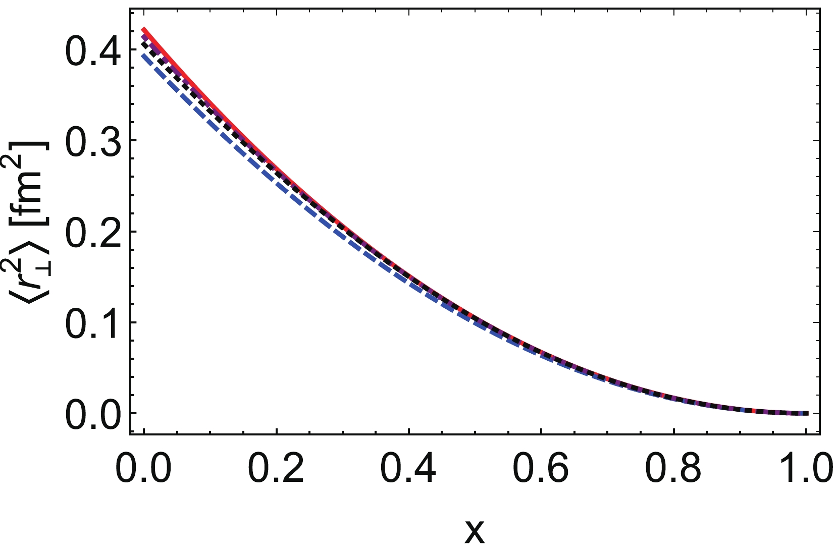
Figure 24. (color online) Width distribution of u quark in the pion for a given momentum fraction x defined in Eq. (38) using different regularization schemes: red line – PT regularization, blue dashed line – 3D regularization, purple dotdashed line – 4D regularization, black dotted line – PV regularization.
$\langle {\boldsymbol{b}}_{\bot}^2\rangle_{\pi}^u$ 

$\langle b_{\bot}^y\rangle_1^u$ 

$\langle b_{\bot}^y\rangle_2^u$ 

$r_{E,LC}$ 

$r_{c,LC}$ 

$r_{c,LC}^D$ 

PT 0.140 0.106 0.071 0.188 0.374 0.513 3D 0.131 0.098 0.066 0.182 0.362 0.472 4D 0.138 0.103 0.069 0.187 0.371 0.476 PV 0.137 0.103 0.069 0.186 0.371 0.482 Table 6. Mean-squared
$\langle {\boldsymbol{b}}_{\bot}^2\rangle_{\pi}^u $ , the average transverse shift$\langle b_{\bot}^y\rangle_n^u$ , the light-cone energy radius and the light-cone charge radius. The mean-squared$\langle {\boldsymbol{b}}_{\bot}^2\rangle_{\pi}^u $ are in units of fm2, the left quantities are in units of fm. -
In this paper, we calculated the pion GPDs in the NJL model using different regularization schemes, including the proper time regularization scheme, 3D momentum cutoff, 4D momentum cutoff, and PV regularization scheme.
First, we plot the diagrams of GPDs, both vector and tensor GPDs are continuous but not differentiable at
$ x=\pm \,\xi $ except$ \xi=0 $ , at this point, GPDs are not continuous. When considering the dressed quark photon vertex and the contact contribution term, vector GPD would be not continuous because of the contact contribution term. The contribution of contact term was not only the discontinuity of vector GPD, but also contributed to$ A_{2,2} $ , it made the value of$ |A_{2,2}(0)| $ approximate$ A_{2,0}(0) $ , if we did not consider the contact contribution term, the two values were quite different, when considering the contact contribution term, they were approximate.Second, we calculated the pion PDFs and plot the diagrams of PDFs from vector GPDs with different
$ m_{\pi} $ , in the chiral limit$ m_{\pi}=0 $ , pion PDF was constant one, when$ m_{\pi}=0.14\,\rm{GeV} $ , in the NJL model PDFs floated around one, when we set$ m_{\pi}= 0.4, 0.6, 0.75 $ GeV, in 4D and 3D regularization schemes, the peaks were sharper than PT and PV regularization schemes. That's because of the factor$ \sigma_1=(M^2-x(1-x)m_{\pi}^2) $ in the PDFs, when M was not large but$ m_{\pi} $ became too large, this term would be negative, then the result would be not right, so we choose a large value of constituent quark mass$ M\approx 0.4 $ GeV, then the maximum value of pion mass was chosen as$ m_{\pi}= 0.75 $ GeV. In 4D and 3D regularization schemes the values of the constituent quark mass were smaller than in PT and PV regularization schemes, so the values of$ \sigma_1 $ in those two schemes were closer to zero, so the peaks of PDFs were sharper and the values were larger.Third, we calculated the FFs from vector GPDs and tensor GPDs and plot the diagrams. For the electromagnetic factors, the bare charge radius from different regularization schemes were close, but for the dressed charge radius in PT regularization scheme was closer to the experiment value
$ r_{\pi}=0.66 $ fm. This was seen in Fig. 20,$ A_{1,0}^{D,\rm{PT}} $ was softer than FFs in other regularization schemes. The gravitational FFs$ A_{2,0}^{\rm{PT}} $ and$ A_{2,2}^{\rm{PT}} $ were also softer than in other regularization schemes. The tensor FFs$ B_{1,0} $ and$ B_{2,0} $ were different from the vector case, they were almost parallel lines, the tensor FFs in 3D regularization scheme were the smallest.Fourth, we study the PDFs in impact parameter space, which were the Fourier transform of GPDs. We plot the diagrams of
$ x*u(x,{\boldsymbol{b}}_{\perp}^2) $ and$ x*u_{\rm{T}}(x,{\boldsymbol{b}}_{\perp}^2) $ , the diagrams in different regularization schemes were similar, there's little difference in values. The width distribution of u quark in the pion were plotted in Fig. 24, they all satisfied the requirement that when$ x\rightarrow 1 $ ,$ H(x,0,-{\boldsymbol{q}}_{\bot}^2) $ should be independent of$ -{\boldsymbol{q}}_{\bot}^2 $ , the struck quark became closer to the centre of momentum since its weight increases, the average impact parameter become zero. The mean-squared$ \langle {\boldsymbol{b}}_{\bot}^2\rangle_{\pi}^u $ were calculated. When quark polarized in the light-front-transverse$ +\,x $ direction, the transverse-spin density was not symmetric around${\boldsymbol{b}}_{\bot}=(b_x=0, $ $ b_y=0)$ anymore, the peaks shift to$ (b_x=0,b_y>0) $ . The average transverse shift$ \langle b_{\bot}^y\rangle_1^u $ and$ \langle b_{\bot}^y\rangle_2^u $ in PT regularization scheme were the largest, in the 3D momentum cutoff were the smallest, the mean-squared$ \langle {\boldsymbol{b}}_{\bot}^2\rangle_{\pi}^u $ are similar.Now, we have arrived at the following conclusion: pion GPDs in the NJL model using different regularization schemes were similar; when considering the contact contribution term, the vector GPD was not continuous at
$ x=\pm \,\xi $ ; and the FFs in the impact parameter space were analogous. The average transverse shift in PT regularization scheme were the biggest, in the 3D momentum cutoff were the smallest. The light-cone energy radius and the light-cone charge radius were similar. In all the regularization schemes, we choose a large constituent quark mass$ M\approx 0.4 $ GeV to avoid$ (M^2-x(1-x)m_{\pi}^2) $ became negative when we choose a large$ m_{\pi} $ in the PDFs. For the choices of parameter sets we referred to Ref. [76], in Tables 1–4 they gave parameter sets in the four different regularization schemes, we tried to use different parameter sets in the same regularization scheme, the diagrams of pion GPDs were almost the same, the cutoff parameter Λ varied from 0.6 GeV to 1.4 GeV, so our results of GPDs were stable. -
We are grateful for constructive comments and technical assistance from Zhu-Fang Cui.
-
Here we use the gamma-functions (
$ n\in \mathbb{Z} $ ,$ n\geq 0 $ )$ \begin{aligned}[b] {\cal{C}}_0(z):=&\int_0^{\infty} {\rm{d}}s\, s \int_{\tau_{uv}^2}^{\tau_{ir}^2} {\rm{d}}\tau \, {\rm e}^{-\tau (s+z)} \\ =&z[\Gamma (-1,z\tau_{uv}^2 )-\Gamma (-1,z\tau_{ir}^2 )]\,, \end{aligned}\tag{A1a} $

$ {\cal{C}}_n(z):=(-)^n\frac{z^n}{n!}\frac{{\rm{d}}^n}{{\rm{d}}\sigma^n}{\cal{C}}_0(z)\,,\tag{A1b} $

$ \bar{\cal{C}}_i(z):=\frac{1}{z}{\cal{C}}_i(z), \tag{A1c}$

where
$ \tau_{uv,ir}=1/\Lambda_{\rm{UV},\rm{IR}} $ are the infrared and ultraviolet regulators, respectively, with$ \Gamma (\alpha,y ) $ being the incomplete gamma-function. z represent the σ functions in the following.The σ functions are define as
$ \sigma_1=M^2-x(1-x)m_{\pi}^2\,, \tag{A2a}$

$ \sigma_2=M^2-x(1-x)t=M^2+x(1-x)Q^2\,, \tag{A2b}$

$ \sigma_3=M^2-\frac{x+\xi}{1+\xi} \frac{1-x}{1+\xi} m_{\pi}^2\,,\tag{A2c} $

$ \sigma_4=M^2-\frac{x-\xi}{1-\xi}\frac{1-x}{1-\xi} m_{\pi}^2\,, \tag{A2d}$

$ \sigma_5=M^2-\frac{1}{4}\left(1+\frac{x}{ \xi }\right)\left(1-\frac{x}{\xi }\right) t\,,\tag{A2e} $

$ \begin{aligned}[b] \sigma_6=&M^2-\alpha \left(1-\alpha \right) m_{\pi}^2 \\ & -\left(\frac{\xi+x}{2\xi}-\alpha \frac{1+\xi}{2\xi}\right) \left(\frac{\xi-x}{2\xi}+\alpha \frac{1-\xi}{2\xi}\right) t\,, \end{aligned} \tag{A2f}$

$ \sigma_7=(x+y)(x+y-1)m_{\pi }^2-xyt+M^2\,,\tag{A2g} $

$ \sigma_8=M^2+(1-\alpha-x) \alpha {\boldsymbol{q}}_{\perp}^2-x \left(1-x\right) m_{\pi}^2.\tag{A2h} $

Regularization dependence of pion generalized parton distributions
- Received Date: 2021-12-07
- Available Online: 2022-06-15
Abstract: Pion generalized parton distributions are calculated within the framework of the Nambu–Jona-Lasinio model using different regularization schemes, including the proper time regularization scheme, the three-dimensional (3D) momentum cutoff scheme, the four-dimensional momentum cutoff scheme, and the Pauli-Villars regularization scheme. Furthermore, we check the theoretical constraints of pion generalized parton distributions required by the symmetries of quantum chromodynamics in different regularization schemes. The diagrams of pion parton distribution functions are plotted, in addition, we evaluate the Mellin moments of generalized parton distributions, which are related to the electromagnetic and gravitational form factors of pion. Pion generalized parton distributions are continuous but not differential at


 DownLoad: