


 Abstract
 HTML
HTML Reference
 Related
 PDF
PDF


-
One of the prime targets of heavy-ion collision experiments at the Large Hadron Collider (LHC), Relativistic Heavy Ion Collider (RHIC) [1–5], and the forthcoming Facility for Antiproton and Ion Research (FAIR) in Darmstadt is to explore the properties of strongly interacting matter, and thus, investigate the different regimes of Quantum Chromo Dynamics (QCD) phase diagrams by varying the collision energy,
$ \sqrt s_{nn} $ . The study of different experimental observables produced in heavy-ion collision experiments play a significant role in understanding the properties of strongly interacting matter at extreme temperatures and densities [6–9]. Quanutm Chromo Dynamics (QCD) suggests that at high baryonic densities and high temperatures, hadrons undergo a phase change to quark-gluon plasma (QGP) [10–14]. Each point on the QCD phase diagram signifies a stable thermodynamic state, which is associated with various thermodynamic functions [15]. Investigating the properties of matter in extreme density and temperature conditions can serve as an important tool to analyze thermal media created a few microseconds after the big-bang [16], study the structure of compact stars [17], and explain the results of heavy-ion collision experiments. The lattice QCD is formulated on grid points of space and time for the study of hadron properties [18, 19].Lattice QCD simulations have suggested that the transition from hadronic to partonic state is a smooth crossover at zero-value of baryon chemical potential,
$ \mu_B $ , and transition temperature,$ T_c $ [20]. As a consequence of QCD fermion sign problem, Monte-Carlo simulations on the lattice are not achievable for$ \mu_B > 0 $ [19, 21]. Another possible approach is using chiral effective models for QCD that have been employed successfully for many years to explore the QCD phase structure [22, 23]. At non-zero values of$ \mu_B $ , this phase transition occurs at relatively lower temperatures (T<160 MeV), but the exact nature of this phase transition and the existence of a probable critical end point (CEP) in the QCD phase diagram is still a point of discussion [24, 25]. Based on the theoretical calculations, a suggestion is that chiral condensates go through first-order phase transitions at non-zero chemical potential, hence the QCD critical point is anticipated to exist. The purpose of the Beam Energy Scan (BES) Program Phase I at RHIC was to search for threshold energies for the QGP signatures and determination of the QGP critical point. The$ p_T $ spectra at mid-rapidity and the kinetic and thermal freeze-out parameters in energy range from 7.7 to 39 GeV with Au-Au collisions were studied in detail. The results at the top RHIC energies have indicated the formation of the phase with partonic degrees of freedom [26]. Beam Energy Scanning Phase II (BES-II) was launched in February of 2019 with the aim to study phase diagrams and critical point locations with high precision [27]. The enhancement of strangeness and suppression of J/$ \Psi $ in nucleus-nucleus collisions were proposed as a strong evidence for the formation of QGP [28].The main goal of experiments and theorists is to develop appropriate tools and observables that can provide an unambiguous signal for the existence of the phase transitions and their universal properties. The idea to scrutinize event-by-event fluctuations of critical end point signatures was initially suggested in [29]. They proposed that a combination of observables including suppressed fluctuations in T and μ, along with enhanced fluctuations in the multiplicity of soft pions, would provide information about location and critical end point properties. Fluctuations of conserved charges, baryon number, strangeness number, and charge number are predicted to be enhanced near the critical-point [30], and hence are identified as absolute observables to confirm its position and existence in the QCD phase diagram. These fluctuations also provide signals for nearby singularities, which are related to chiral limit at low values of baryon number in the QCD phase diagram. Higher order of conserved quantity cumulants can be determined from heavy ion collisions experiments by performing event-by-event analysis and are compared with theoretical ideas to provide stronger evidence of a CEP. Analysis of these conserved quantity susceptibilities, both experimentally and theoretically, provide insight about pertinent degrees of freedom, as well as locate a critical point in the phase diagram. In the quest of determining the freeze-out conditions, many statistical hadronization models and hadron resonance gas models use the experimentally determined particle yields and ratios as input [31, 32]. The experimental results at different collision energies for these variables have already been presented [33, 34]. Additionally, the matter formed in heavy-ion collisions goes through several stages and is not permanently in equilibrium.
In order to understand the various regimes of a QCD phase diagram, many theoretical models have been proposed. Linear sigma model (LSM) [35], non-linear sigma model, and Walecka model [model [36] were the earliest models and were extended later through models like the Nambu-Jona-Lasinio (NJL) model [37]. Different theoretical approaches like the chiral hadronic model [38], hadron resonance gas (HRG) model [39], Polyakov-quark-meson (PQM) model [40], Dyson-Schwinger equation framework [41], Nambu-Jona-Lasinio (NJL) model [42], Polyakov NJL (PNJL) model [43], and functional renormalization group (FRG) [40] approach have been used to analyze the fluctuations of conserved charges. These chiral models are based on two key properties of QCD, namely confinement and asymptotic freedom. Chiral effective models have been used to reproduce important thermodynamic properties by mean-field approximations. Although various chiral models are an effective tool to explore the QCD phase diagram, they do not include deconfinement. Also, inclusion of any form of the Polyakov loop modifies the model parameters to give good results at vanishing density. Thus Polyakov-loop potential incorporates the gluonic degrees of freedom to provide a better understanding of strongly interacting matter.
In this study, we used the PQM model and Polyakov loop extended chiral quark mean field (PCQMF) model to study isospin asymmetric quark matter at finite density and temperature. The Polyakov loop extended models were employed to study the thermodynamic properties of quark matter as well as susceptibilities of conserved charges. In the PCQMF model, we calculated the value of the non-strange scalar field (σ), strange scalar meson field (ζ), scalar isovector meson field (δ), scalar isoscalar dilaton field (χ), non-strange vector field (ω), non-strange vector-isovector field (ρ), and strange vector field (ϕ) at finite temperatures and densities. In the PQM model, quark condensates,
$ \sigma_u $ ,$ \sigma_d $ , and$ \sigma_s $ , and different vector fields have been studied in isospin asymmetric matter. In earlier studies, the three-flavored quark-meson model has been employed to study the equation of state and phase diagram with the inclusion of vector interactions by using the mean-field approach [44]. The two-flavored PQM model based on the functional renormalization group (FRG) method has been applied to calculate quark number fluctuations and higher order moments [40]. Along with the modelling of vector meson interactions, by extending the quark-meson model through introducing the Polaykov-loop potential, the properties of both deconfinement and chiral symmetry breaking may be studied. Thermodynamical quantities like pressure, entropy, and energy density can be derived by using the expression for thermodynamic potential. Both these models are based on the mean field approximation and are used to explain many-body interactions. Many theoretical studies use the Taylor series expansion to calculate cumulants of conserved charge net fluctuations [45]. The curvature of the transition line and the radius of convergence of the Taylor series for baryon number fluctuations at finite values of baryonic chemical potential for a (2+1)-flavor model was calculated in Schmidt, et al. [39].This paper is organized as follows. In Sec. II.A, we briefly describe the quark meson model and obtained the grand canonical potential. In Sec. II.B, we discuss the chiral SU(3) quark mean-field model and its thermodynamics. In Sec. II.C, we describe the Polyakov loop potential. In Sec. II.D, the Taylor series method is discussed in detail for description of cumulants and hence susceptibilities. In Sec. III, a descriptive view of all the results for asymmetric quark matter and fluctuations is presented. In Sec. IV, we summarize the results for the study
-
The chiral quark meson model effectively incorporates the properties of a low-energy QCD. The order parameter of the chiral phase transition in the limit of massless quarks is quark condensate. But due to existence of quark mass in the real world, chiral symmetry is broken explicitly, as well as spontaneously, in a vacuum, and hence confinement properties are not explained well in the QM model. Thus, by combining Polyakov loop potential in the model, both confinement and chiral properties of the QCD are well explained. The effective Lagrangian of the quark meson model incorporating the coupling of quarks and mesons based on the linear sigma model with the linear sigma model with
$ N_f $ flavors is given by [44, 46]$ \begin{aligned}[b] {\cal{L}} =& \bar{\psi}{\rm i} \gamma^{\mu}{\partial}_{\mu} \psi + {\rm{Tr}}\left(\partial_{\mu} \varphi^{\dagger} \partial^{\mu} \varphi\right)- m^{2} {\rm{Tr}}\left(\varphi^{\dagger} \varphi\right) \\&- \lambda_{1}\left[{\rm{Tr}}\left(\varphi^{\dagger} \varphi\right)\right]^{2} -\lambda_{2}\left[{\rm Tr}\left(\varphi^{\dagger} \varphi\right)\right]^{2} \\&+ c\left({\rm{det}}(\varphi)+{\rm{det}}\left(\varphi^{\dagger}\right)\right) + {\rm{Tr}}\left[H\left(\varphi+\varphi^{\dagger}\right)\right] \\& + {\cal{L}}_{qm} -\frac{1}{4}{\rm{Tr}}\left(V_{ \mu \nu }V^{ \mu \nu }\right) + \frac{m_1^2}{2}V_{a \mu} V_{\mu}^a, \end{aligned} $

(1) where,
$ \begin{equation} \varphi = T_{a} \varphi_{a} = T_{a}\left(\sigma_{a}+{\rm i} \gamma_{5} \pi_{a}\right). \end{equation} $

(2) The quark spinor for
$ N_f $ is ψ =$ (u,d,s) $ , and$ N_c $ = 3 for color degrees of freedom. Gell-Mann matrices given by$ T_a = \lambda_a/2 $ are generators of the U($ N_f $ ) symmetry group with$ a = 0,\cdots,N_{f}^2 - 1 $ . In the effective Lagrangian, the first term represents the kinetic energy part of massless quarks, and second and third terms are standard kinetic energy and mass term for scalar mesons, respectively. The fourth and fifth terms are the quadratic interaction terms involving coupling constants, ants,$ \lambda_1 $ and$ \lambda_2 $ . The next terms are the cubic coupling terms between the fields, which corresponds to the$ U(1)_A $ anomaly and explicit symmetry breaking term expressed by$ H = T_{a}h_a $ . The$ {\cal{L}}_{\rm qm} $ is the quark mesons interaction term and is given as [47]$ \begin{equation} {\cal{L}}_{\rm q m} = g_{s}\left(\bar{\psi}_{\rm L} \varphi \psi_{\rm R}+\bar{\psi}_{\rm R} \varphi^{\dagger} \psi_{\rm L}\right)-g_{v}\left(\bar{\psi}_{\rm L} \gamma^{\mu} L_{\mu} \psi_{\rm L}+\bar{\psi}_{\rm R} \gamma^{\mu} R_{\mu} \psi_{\rm R}\right), \end{equation} $

(3) where
$ g_s $ and$ g_v $ are scalar and vector meson coupling constants, respectively. Since the effective Lagrangian of the quark-meson model has$SU(3)_{\rm L} \times SU(3)_{\rm R}$ symmetry, the generators of group are vector and axial charges. The standard model is extended by inclusion of the vector meson contribution where vector meson interactions with quarks give a repulsive contribution, while the attractive contribution is provided by interaction of quarks with scalar mesons. In the last line of Eq. (1),$ V_{ \mu \nu} $ is the field tensor corresponding to vector mesons. The second term in this line is the kinetic energy term, and the third is the mass term of vector mesons. Spin-1 mesons defined in terms of vector ($ V_{\mu}^a $ ) and pseudovector mesons ($ A_{\mu}^a $ ) nonets are [46]$ \begin{eqnarray} L_{\mu}\left(R_{\mu}\right) = \frac{1}{2}\left(V_{\mu} \pm A_{\mu}\right) = \sum\limits_{a = 0}^{8}\left(V_{\mu}^{a} \pm A_{\mu}^{a}\right) T_{a}. \end{eqnarray} $

(4) Expressions for
$ V_{\mu} $ and$ A_{\mu} $ have been given in the appendix. In order to calculate the constituent quark masses due to spontaneous breaking of chiral symmetry, we used a (2+1) Quark-Meson model. The self-interaction potential of meson fields in terms of quark condensates is given as[48]$ \begin{aligned}[b] U\left(\sigma_{u}, \sigma_{d}, \sigma_{s}\right) =& \frac{\lambda_{1}}{4}\left[\left(\frac{\sigma_{u}^{2}+\sigma_{d}^{2}}{2}\right)^{2}+\sigma_{s}^{4}+ \left(\sigma_{u}^{2}+\sigma_{d}^{2}\right) \sigma_{s}^{2}\right] \\&+ \frac{\lambda_{2}}{4}\left(\frac{\sigma_{u}^{4}+\sigma_{d}^{4}}{4}+ \sigma_{s}^{4}\right)-\frac{c}{2 \sqrt{2}} \sigma_{u} \sigma_{d} \sigma_{s} \\&+ \frac{m^{2}}{2}\left(\frac{\sigma_{u}^{2}+\sigma_{d}^{2}}{2}+\sigma_{s}^{2}\right)- \frac{h_{u d}}{2}\left(\sigma_{u}+\sigma_{d}\right)-h_{s} \sigma_{s} . \end{aligned} $

(5) The isospin symmetry of the QCD is not broken in a vaccum, which is proven by the Vafa-Witten theorem [49], and hence,
$ h_{ud} $ gives the explicit symmetry breaking for both up and down quarks. At zero values of chemical potential and temperature, there is a contribution only from the vaccum term, which is usually neglected. Contribution of quark-antiquark interactions in a thermodynamic potential is given as [50]$ \begin{equation} \Omega_{q\bar{q}} = \Omega_{q\bar{q}}^{v}+\Omega_{q \bar{q}}^{\rm t h}, \end{equation} $

(6) where,
$ \begin{equation} \Omega_{q\bar{q}}^{v} = -2 N_{c} \sum\limits_{f = u,d,s} \int \frac{{\rm d}^{3} p}{(2 \pi)^{3}} E_{f} \;\;\; \end{equation} $

(7) $ \begin{aligned}[b] \Omega_{q\bar{q}}^{\rm th} = -\frac{1}{2}(m_{\omega}^{2}\omega^2 + m_{\rho}^2 \rho^2 + m_{\phi}^{2}\phi^2) \end{aligned} $

$ \begin{aligned}[b] \quad - 2 T \sum\limits_{f = u, d, s} \int \frac{{\rm d}^{3} p}{(2 \pi)^{3}}\left[\ln g_{f}^++\ln g_{f}^-\right]. \end{aligned} $

(8) In above equation,
$ g_{f}^{+} $ and$ g_{f}^{-} $ are defined as$ g_{f}^+ = \left[1+3 \Phi {\rm e}^{-(E_f-\mu_f)/ T}+3 \bar{\Phi} {\rm e}^{-2(E_f-\mu_f) / T}+{\rm e}^{-3(E_f-\mu_f)/ T}\right]$

(9) and
$ \begin{equation} g_{f}^- = \left[1+3\bar\Phi {\rm e}^{-(E_f+\mu_f)/ T} +3 \Phi {\rm e}^{-2(E_f+\mu_f)/ T} +{\rm e}^{-3(E_f+\mu_f)/ T}\right]. \end{equation} $

(10) In Eq. (8),
$ \Omega_{q\bar{q}}^{\rm th} $ gives the thermal fluctuation contribution from antiquarks and quarks due to interaction of meson fields and Polyakov-loop variables. Also, ω is the non-strange vector field, ρ is the non-strange vector-isovector field, and ϕ is the strange vector field. Considering the asymmetric matter, we defined the effective chemical potential ($ \nu_i^{*} $ ) for individual quarks in terms of isospin chemical potential and quark chemical potential, potential,$ \mu_q = \mu_B/3 $ , where$ \mu_B $ is baryonic chemical potential through relations,$ \begin{aligned}[b] \nu_u^{*} =& \mu_q + \frac{2}{3} \mu_Q - g_{\omega u} \omega - g_{\rho u}\rho, \\ \nu_d^{*} =& \mu_q - \frac{1}{3}\mu_Q - g_{\omega d} \omega + g_{\rho d}\rho , \\ \nu_s^{*} = &\mu_q -\frac{1}{3}\mu_Q -\mu_S - g_{\phi s}\phi. \end{aligned} $

(11) Due to vector interaction, there is a shift in the quarks effective chemical potential [51]. The single particle energy of quarks is given by
$ E_f^{*} = \sqrt{k^2 + m_{i}^{*2}} $ , where constituent quark masses is represented as$ \begin{equation} m_u^{*} = \frac{g}{2}\sigma_u,\quad m_d^{*} = \frac{g}{2}\sigma_d,\; and \quad m_s^{*} = \frac{g}{\sqrt{2}}\sigma_s. \end{equation} $

(12) In above equation, g represents the Yukawa coupling constant. After applying dimensional regularization to the vacuum term in Eq. (7), we got [52]
$ \begin{equation} \Omega^{v}_{q\bar{q}} = \Omega_{q\bar{q}}^{\mathrm{reg}}(\Lambda) = -\frac{N_{c}}{8 \pi^{2}} \sum\limits_{f = u, d, s} m_{f}^{4} \log \left[\frac{m_{f}}{\Lambda}\right], \end{equation} $

(13) Here, Λ is the regularization scale parameter. Skokov, et al. concluded [53] that the inclusion of the fermion vacuum term in the quark meson model influences the phase transition in the chiral limit. Considering all the terms discussed above, the total thermodynamic potential is given as
$ \begin{aligned}[b]& \Omega\left(\sigma_{u}, \sigma_{d}, \sigma_{s},\omega, \rho, \phi, \Phi,\bar{\Phi}; T, \mu_{f}\right) \\=& U\left(\sigma_{u}, \sigma_{d}, \sigma_{s}\right) + \Omega_{q \bar{q}}^{\rm v a c}\left(\sigma_{u}, \sigma_{d}, \sigma_{s}\right) + {\cal{U}}\left(\Phi,\bar{\Phi}: T, \mu_{f}\right) \\&+ \Omega_{q \bar{q}}^{\rm t h}\left(\sigma_{u}, \sigma_{d}, \sigma_{s}, \omega, \rho, \phi, \Phi,\bar{\Phi}: T, \mu_{f}\right), \end{aligned} $

(14) where
$ {\cal{U}}(\Phi,\bar\Phi: T, \mu_{f}) $ is the Polyakov loop potential. Now we minimize the derived thermodynamic potential to obtain equations of motion as$ \begin{aligned}[b] \frac{\partial \Omega}{\partial \sigma_u} = &\frac{\partial \Omega}{\partial \sigma_d} = \frac{\partial \Omega}{\partial \sigma_s} = \frac{\partial \Omega}{\partial \omega} = \frac{\partial \Omega}{\partial \rho} \\=& \frac{\partial \Omega}{\partial \phi} = \frac{\partial \Omega}{\partial \Phi} = \frac{\partial \Omega}{\partial \bar {\Phi}}. \end{aligned} $

(15) The field equations were derived by solving the above expression and the details are given in the appendix.
-
The CQMF model describes the meson-meson and quark-meson interactions based on non-linear realization of chiral SU(3) symmetry [54, 55] and broken scale invariance [54, 56, 57] at finite density and temperature. The Lagrangian for the chiral quark mean field model is given as [47]
$ \begin{equation} {\cal{L}}_{\text{eff}} = {\cal{L}}_{q0}+{\cal{L}}_{qm}+ {\cal{L}}_ {\Sigma\Sigma} + {\cal{L}}_{VV} +{\cal{L}}_{S B}+{\cal{L}}_{\Delta m} + {\cal{L}}_{h} . \end{equation} $

(16) In Eq. (16),
$ {\cal{L}}_{q0} = \bar q \, {\rm i}\gamma^\mu \partial_\mu q $ represents the free part of massless quarks,$ {\cal{L}}_{qm} $ describes the quark mesons interaction,$ {\cal{L}}_{\Sigma\Sigma} $ is the scalar meson self-interaction term,$ {\cal{L}}_{VV} $ is vector meson self-interaction term, and and$ {\cal{L}}_{SB} $ ,$ {\cal{L}}_{\Delta m} $ , and and$ {\cal{L}}_{h} $ are explicit symmetry breaking terms. The interaction between meson and quarks is defined via exchange of vector meson fields, ω, ρ, and ϕ, as well as scalar meson fields, σ, ζ, and δ. The interaction between mesons is described by the equation below:$ \begin{aligned}[b] {\cal{L}}_m =& {\cal{L}}_{VV}+ {\cal{L}}_{\Sigma\Sigma} + {\cal{L}}_{SB} = \frac{1}{2}\frac{\chi^2}{\chi_0^2} \left(m_\omega^2\omega^2+m_\rho^2\rho^2+m_\phi^2\phi^2\right) \\&+ g_4\left(\omega^4+6\omega^2\rho^2+\rho^4+2\phi^4\right) \\& -\frac{1}{2} k_0 \chi^2 \left(\sigma^2+\zeta^2+\delta^2\right)+k_1 \left(\sigma^2+ \zeta^2+\delta^2\right)^2 \\& +k_2(\frac{\sigma^4}{2} +\frac{\delta^4}{2}+3\sigma^2\delta^2+\zeta^4) +k_3\chi\left(\sigma^2-\delta^2\right)\zeta \\& -k_4\chi^4-\frac14\chi^4 {\rm{ln}}\frac{\chi^4}{\chi_0^4} + \frac{d} 3\chi^4 {\rm{ln}}\left(\left(\frac{\left(\sigma^2-\delta^2\right)\zeta}{\sigma_0^2\zeta_0}\right)\left(\frac{\chi^3}{\chi_0^3}\right)\right) \\& -\frac{\chi^2}{\chi_0^2}\left[m_\pi^2f_\pi\sigma + \left(\sqrt{2}m_K^2f_K-\frac{m_\pi^2}{\sqrt{2}}f_\pi\right)\zeta\right]. \end{aligned} $

(17) In Eq. (17),
$ {\cal{L}}_{VV} $ is the self-interaction term for vector mesons,$ {\cal{L}}_{\Sigma\Sigma} $ is the mesonic self-interaction term, and$ {\cal{L}}_{SB} $ is due to chiral symmetry breaking [58–61]. The strange scalar isoscalar field, ζ gives a description of strange matter in the model, whereas the scalar isovector field, δ recounts for isospin asymmetric matter in mean-field models. The last two terms of Eq. (16) also contribute to chiral symmetry breaking and are written as$ \begin{eqnarray} {\cal{L}}_{\Delta m} = - \Delta m_s \bar q S q \;\;\end{eqnarray} $

(18) $ \begin{eqnarray} {\cal{L}}_h \, = \, (h_1 \, \sigma \, + \, h_2 \, \zeta) \, \bar{s} s \, . \end{eqnarray} $

(19) The partial conserved axial vector current equations for K- and π-mesons are satisfied due to the non-zero divergence of axial currents. The precise constituent mass of quarks is determined by the inclusion of
$ {\cal{L}}_{\Delta m} $ as the mass term where here$ S \, = \, \dfrac{1}{3} \, \left(I - \lambda_8\sqrt{3}\right) = {\rm{diag}}(0,0,1) $ is the strangeness quark matrix, and$ \Delta m_s = 29 $ MeV. The total thermodynamic potential of PCQMF is given as$ \begin{eqnarray} &&\Omega = {\cal{U}}(\Phi,\bar{\Phi},T) +\Omega_{q\bar{q}}-{\cal{L}}_M- {\cal{V}}_{\rm vac}, \end{eqnarray} $

(20) where
$ {\cal{U}}(\Phi,\bar{\Phi},T) $ is the Polyakov loop potential term,$ {\cal{L}}_M $ is the mesonic interaction term given as$ {\cal{L}}_M = {\cal{L}}_{\Sigma\Sigma} +{\cal{L}}_{VV} +{\cal{L}}_{SB} $ ,$ {\cal{V}}_{\rm vac} $ is vaccum energy term, and$ \Omega_{q\bar{q}} $ is the contribution of quarks and antiquarks. The effective chemical potential of quarks in the presence of vector fields is related to the original chemical potential as described in Eq. (11). The effective constituent masses of quarks is given as$ \begin{equation} {m_i}^{*} = -g_{\sigma i}\sigma - g_{\zeta i}\zeta - g_{\delta i}\delta + {m_{i0}}. \end{equation} $

(21) Here,
$ g_{\sigma i} $ ,$ g_{\zeta i} $ , and$ g_{\delta i} $ represent the coupling strengths of quarks with scalar fields. The values of$ g_{\sigma i} $ ,$ g_{\zeta i} $ , and$ {m_{i0}} $ are obtained by fitting the vacuum masses of constituent quarks, which are considered to be$ m_u = m_d = 313 $ MeV and$ m_s = 490 $ MeV [62]. In order to find the values of the scalar fields, σ, ζ and δ, the dilaton field, χ, the vector fields, ω, ρ, and ϕ, and the Polyakov field, Φ, and its conjugate,$ \bar{\Phi} $ , total thermodynamic potential, Ω, is minimized with respect to these fields,$ {\rm i.e.} $ , we obtain$ \begin{aligned}[b] \frac{\partial\Omega} {\partial\sigma} =& \frac{\partial\Omega}{\partial\zeta} = \frac{\partial\Omega}{\partial\delta} = \frac{\partial\Omega}{\partial\chi} = \frac{\partial\Omega}{\partial\omega} = \frac{\partial\Omega}{\partial\rho}\\ =& \frac{\partial\Omega}{\partial\phi} = \frac{\partial\Omega}{\partial\Phi} = \frac{\partial\Omega}{\partial\bar\Phi} = 0. \end{aligned} $

(22) The equations obtained after solving the above equations are mentioned in the appendix. The equations for the Polyakov-loop variables is same for both the PQM and PCQMF models. These equations were derived by using the form of the Polyakov-loop mentioned in Sec. II.C. By solving the above coupled equations, we obtained other thermodynamic properties of the model. The total baryon density is given as
$ \rho_B = \dfrac{1}{3} (\rho_u+\rho_d+\rho_s) $ . In order to study the asymmetric quark matter, we introduced the isospin asymmetry by defining$ \begin{equation} \eta = \frac{(\rho_d-\rho_u)}{(\rho_d+\rho_u)/3}. \end{equation} $

(23) -
One of the most important observables in a finite-temperature QCD is the Polyakov loop. In the infinite mass limit of quarks, its expectation value determines the order parameter, which contributes to confinement. The Polyakov loop operator is defined as a Wilson loop in temporal direction and is written as
$ \begin{equation} {\cal{P}}(\vec{x}) = {\cal{P}} {\rm exp}\bigg[{\rm i}\int_0^{\beta} {\rm d}\tau A_0 (\vec{x},\tau) \bigg]. \end{equation} $

(24) Here,
$ {\cal{P}} $ represents path-ordering, and$ A_0 (\vec{x},\tau) $ gives the temporal component for the Euclidean gauge field [63–66]. The order parameter for$ Z(N_{\rm C}) $ fo symmetry breaking in terms of the thermal Wilson line is given as [67]$ \begin{equation} A_\mu = {\rm i}g_sA_\mu^{w}\frac{\lambda_w}{2}\delta_0^\mu, \; \; \; \; \; \; \;\; w = 1,....{N^{2}_{\rm C}}-1. \end{equation} $

(25) In the above equation,
$ A_{\mu}^w $ is the gluon field with color index a. The Polyakov loop variables, Φ, and its conjugate,$ \bar\Phi $ , are given as$ \begin{aligned}[b] \Phi(\vec{x}) = &({\rm Tr}_c L)/N_{\rm C} \; \\ \bar{\Phi}(\vec{x}) =& ({\rm Tr}_c L^\dagger)/N_{\rm C}. \end{aligned} $

(26) There is no unique choice of the Polyakov loop potential and the solution depends on the center symmetry of the pure-gauge theory. The different parameters for different forms of Polyakov-loop potentials can be calculated by using the pure gauge lattice data at zero-value chemical potential [68]. The polynomial parametrized form of the Polyakov-loop potential is represented as [69]
$ \begin{aligned}[b] \frac{{\cal{U}}_{\text {poly }}(\Phi, \bar{\Phi})}{T^{4}} = &-\frac{b_{2}(T)}{2} \bar{\Phi} \Phi-\frac{b_{3}}{6}\left(\Phi^{3}+\bar{\Phi}^{3}\right)\\&+\frac{b_{4}}{4}(\bar{\Phi} \Phi)^{2}, \end{aligned} $

(27) with the temperature-dependent coefficient,
$ b_{2} $ , defined as$ \begin{equation} b_{2}(T) = a_{0}+a_{1}\left(\frac{T_{0}}{T}\right)+a_{2}\left(\frac{T_{0}}{T}\right)^{2}+a_{3}\left(\frac{T_{0}}{T}\right)^{3} . \end{equation} $

(28) The parameters determined to fit the lattice simulations for the polynomial form of the Polyakov-loop were:
$ a_0 = 1.53 $ ,$ a_1 = 0.96 $ ,$ a_2 = -2.3 $ ,$ a_3 = -2.85 $ ,$ b_3 = 13.34 $ , and$ b_4 = 14.88 $ . The logarithmic form of the Polyakov-loop potential is written as [70, 71]$ \begin{aligned}[b] \frac{U(\Phi,\bar{\Phi},T)}{T^4} =& -\frac{a(T)}{2}\bar{\Phi}\Phi+b(T)\mathrm{ln}\big[1-6\bar{\Phi}\Phi \\&+ 4(\bar{\Phi}^3+\Phi^3)-3(\bar{\Phi}\Phi)^2\big], \end{aligned} $

(29) where
$ \begin{equation} a(T) = a_0+a_1\bigg(\frac{T_0}{T}\bigg)+a_2\bigg(\frac{T_0}{T}\bigg)^2,\ \ b(T) = b_3\bigg(\frac{T_0}{T}\bigg)^3, \end{equation} $

(30) here,
$ a_0 $ = 1.81,$ a_1 $ = −2.47,$ a_2 $ = 15.2, and$ b_3 $ = −1.75, which were derived in accordance with the results from the pure gauge QCD.In Schaeffer, et al. [72], the dependence of chiral and deconfinement transition on the chemical potential dependent
$ T_0 $ was investigated, and results were compared for when$ T_0 $ was considered independent of chemical potential. Coinciding transition lines for deconfinement and chiral transition have been obtained within an accuracy of ±5 MeV [72]. In our calculations, we considered a fixed value for the parameter$ T_0 $ . However, we verified the concurrence of deconfinement and the chiral phase transition line when chemical potential dependent$ T_0 $ was considered. By the inclusion of the Polyakov loop potential with the CQMF model, the features of both deconfinement and chiral symmetry breaking can be studied. -
Using the derived thermodynamic potential and solving the gap equations, we can define the relations for pressure, p, entropy density, s, and energy density, ϵ, as
$ \begin{equation} p = -\Omega, \end{equation} $

(31) $ \begin{equation} s = -\frac{\partial \Omega}{\partial T}, \end{equation} $

(32) and
$ \begin{equation} \epsilon = \Omega+\sum\limits_{i = u, d, s} {\nu_i}^{*} \rho_i+TS. \end{equation} $

(33) After obtaining pressure, the Taylor series expansion is used to derive derivatives of different order, and hence the susceptibilities of different conserved charges at zero value of corresponding chemical potential. The generalized susceptibilities of conserved charges is given as [43]
$ \begin{equation} \chi^{BQS}_{ijk} = \frac {\partial^{i+j+k} [P/T^{4}]} {\partial \left(\mu_{B}/T \right)^{i} \partial(\mu_{Q}/T)^{j} \partial(\mu_{S}/T)^{k}}. \end{equation} $

(34) We can expand the scaled pressure as [45]
$ \begin{equation} \frac{P(T,\mu_{B})}{T^{4}} = \sum\limits_{n = 0}^{\infty} {c_{n}(T)}\left(\frac{\mu_{B}}{T} \right) . \end{equation} $

(35) The Taylor coefficients of pressure are extracted by expansion around the scaled chemical potential at
$ \mu_{B}/T $ = 0, where odd terms vanish due to charge-parity symmetry. The cumulants obtained from Eq. (35) are related to skewness and kurtosis as$ S\sigma = \frac{C_{3}^{B}}{C_{2}^{B}} = \frac{\chi_{3}^{B}}{\chi_{2}^{B}} $

and
$ \begin{equation} K\sigma^{2} = \frac{C_{4}^{B}}{C_{2}^{B}} = \frac{\chi_{4}^{B}}{\chi_{2}^{B}}. \end{equation} $

(36) The calculations of skewness and kurtosis help in relating chiral and deconfinement transitions to statistical distributions of net-baryon number fluctuations in both the critical and crossover regions. By considering the expansion of Eq. (35) in powers of
$ \mu_B/T $ , we can rewrite the susceptibilities at a finite value of chemical potential as [73]$ \chi_{2}^{B}\left(\mu_{B}\right) \simeq \chi_{2}^{B}(0)+\frac{\chi_{4}^{B}(0)}{2 !} \left(\frac{\mu_B}{T}\right)^{2}+\frac{\chi_{6}^{B}(0)}{4 !} \left(\frac{\mu_B}{T}\right)^{4} +\frac{\chi_{8}^{B}(0)}{6 !} \left(\frac{\mu_B}{T}\right)^{6}, $

(37) $ \chi_{4}^{B}\left(\mu_{B}\right) \simeq \chi_{4}^{B}(0)+\frac{\chi_{6}^{B}(0)}{2 !} \left(\frac{\mu_B}{T}\right)^{2}+\frac{\chi_{8}^{B}(0)}{4 !} \left(\frac{\mu_B}{T}\right)^{4}, \;\; $

(38) $ X_{6}^{B}\left(\mu_{B}\right) \simeq \chi_{6}^{B}(0)+\frac{\chi_{8}^{B}(0)}{2 !} \left(\frac{\mu_B}{T}\right)^{2}. $

(39) Quark number fluctuations in the two-flavored PQM model at finite chemical potential have been studied via Dyson-Schwinger Equation Approach [74]. Many theoretical models have used automatic-differentiation to obtain higher order cumulants and susceptibilities [50, 75].
-
In this section, we present the results for different thermodynamical variables for the PQM model and the PCQMF model in strange isospin asymmetric quark matter. The model parameters in the PQM model, g,
$ \lambda_1 $ ,$ \lambda_2 $ , c, and m, were determined in a way to reproduce vacuum values for mesons and quarks by fixing momentum cut off,$ \Lambda $ ,at 200 MeV. Parameters for the PQM model are given in Table 1 and those for PCQMF model are given in Table 2 [47]. The value of g was determined from the vacuum mass of light quarks which was taken to be 302 MeV.g $\Lambda_1$ 

$\Lambda_2$ 

$ \Lambda $ 

m c $h_{ud}$ 

$h_s$ 

$f_\pi$ /MeV

$m_\omega = m_\rho/{\rm MeV}$ 

$m_\phi$ /MeV

6.5 −8.165 138.45 200 80647.58 4801.95 1785000 338050000 92.4 770 1019 Table 1. The list of parameters used in the present study for the PQM model.
$k_0$ 

$k_1$ 

$k_2$ 

$k_3$ 

$k_4$ 

$g_s$ 

$g_v$ 

${g_4}$ 

$h_1$ 

$h_2$ 

4.94 2.12 −10.16 −5.38 −0.06 4.76 10.92 37.5 −2.20 3.24 $\sigma_0$ /MeV

$\zeta_0$ /MeV

$\chi_0$ /MeV

$m_\pi$ /MeV

$f_\pi$ /MeV

$m_K$ /MeV

$f_K$ /MeV

$m_\omega$ =

$m_\rho$ /MeV

$m_\phi$ /MeV

d −93 −96.87 254.6 139 93 496 115 783 1020 0.18 $g_{\sigma u}=g_{\sigma d}$ 

$g_{\sigma s}$ =

$g_{\zeta u}$ 

$g_{\zeta s}$ 

$g_{\delta u}$ =−

$g_{\delta d}$ 

$g_{\delta s}$ =

$g_{\zeta d}$ 

$g_{\omega u}$ =

$g_{\omega d}$ 

$g_{\omega s}$ =

$g_{\phi u}$ =

$g_{\phi d}$ 

$g_{\phi s}$ 

$g_{\rho u}$ =−

$g_{\rho d}$ 

$g_{\rho s}$ 

3.36 0 4.76 3.36 0 3.86 0 5.46 3.86 0 Table 2. The list of parameters used in the present study for the PCQMF model.
In Sec. III.A, we discuss the thermodynamic properties of the PQM model at different values of temperature and chemical potential. In Sec. III.B, we study, in detail, the thermodynamics of quark matter within the PCQMF model, and then, a comparative study is conducted on the two models. In the last section, we investigate the susceptibilities of conserved charges for both models.
-
In this section we present the results for isospin asymmetric strange quark matter with the inclusion of vector interactions in the PQM model. The phase structure of the PQM was modified due to the introduction of isospin chemical potential, as well as vector coupling. In this study, we considered the vector coupling constant,
$ g_v $ , as a free parameter defined in terms of$ v = g_v/g $ , which has different values depending upon the vector coupling strength. The phase diagram of the QCD was obtained by studying the behavior of the order parameters.In Fig. 1 and Fig. 2, we show the variation in
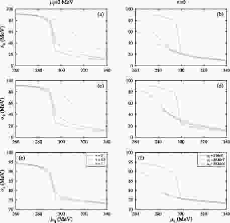
$ \sigma_u $ ,$ \sigma_d $ ,$ \sigma_s $ , Φ, and$ \bar \Phi $ as a function of quark chemical potential ($ \mu_q $ ) for vector coupling ratios, v = 0, 0.5, and 1 in the left panel for$ T_{\rm CP} $ = 72 MeV determined at$ \mu_I $ = 0 MeV and v = 0.5. In the right panel, the order parameters are plotted for isospin chemical potential$ \mu_I $ = 0, 50, and 70 MeV and$ T_{\rm CP} $ = 69 MeV, which were calculated for$ \mu_I $ = 50 MeV and zero value of vector coupling ratio. For lower values of$ \mu_q $ , the values of the order parameters remained almost constant. At zero value of isospin chemical potential and vector coupling ratio, there was a discontinuity for quark chemical potential at ≈ 295 MeV. We showed that at vanishing values of v and$ \mu_I $ , there was a first order chiral phase transition. As the value of vector coupling ratio increased, we got a smooth curve, signifying the change of first-order transition to crossover. Similar change of first-order transition to crossover was observed for all quark condensates and Polyakov-loop variables with changing values of isospin chemical potential. At the higher values of quark chemical potential, there was a difference in value of$ \sigma_u $ and$ \sigma_d $ for due to isospin asymmetry at finite values. With the increase in value of the vector-scalar interaction ratio, the order parameters value moved to higher quark chemical potential. Contrarily, with rise in value of isospin chemical potential, the value of quark condensates and Polyakov loop variables shifted to lower values of quark chemical potential. Hence, the change in coupling ratio, v, and isospin chemical potential,$ \mu_I $ , had the opposite effect on the phase transition line. The change of structure of phase transitions with the higher values of isospin chemical potential and vector coupling has also been shown in [77, 78].
Figure 1. (color online) The order parameters,
$ \sigma_u $ ,$ \sigma_d $ , and$ \sigma_s $ , as a function of quark chemical potential,$ \mu_q $ , for vector coupling ratio, v = 0, 0.5, and 1 (left panel), at zero value of isospin chemical potential for$ T_{\rm CP} $ = 72 MeV (for$ \mu_I $ = 0 MeV, v = 0.5) and for isospin chemical potential,$ \mu_I $ = 0, 50, and 70 MeV (right panel) at zero value of vector coupling ratio, v, for$ T_{\rm CP} $ = 69 MeV (for$ \mu_I $ = 50 MeV, v = 0).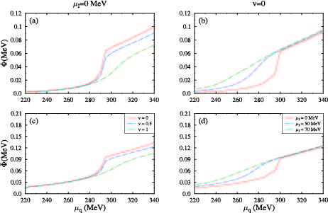
Figure 2. (color online) The order parameters, Φ and
$ \bar\Phi $ , as a function of quark chemical potential,$ \mu_q $ , for vector coupling ratio, v = 0, 0.5, and 1 (left panel), at zero value of isospin chemical potential for$ T_{\rm CP} $ = 72 MeV (for$ \mu_I $ = 0 MeV, v = 0.5) and for isospin chemical potential$ \mu_I $ = 0, 50, and 70 MeV (right panel), at zero value of vector coupling ratio, v, for$ T_{\rm CP} $ = 69 MeV (for$ \mu_I $ = 50 MeV, v = 0).In Fig. 3, we plotted quark condensates,
$ \sigma_u $ ,$ \sigma_d $ , and$ \sigma_s $ (Fig. 4 for Φ and$ \bar\Phi $ ) as a function of temperature, T for isospin chemical potential,$ \mu_I $ = 0, 50, 70, and 120 MeV, and strangeness chemical potential,$ \mu_S $ = 0, and 200 MeV for baryonic chemical potential fixed at$ \mu_B $ = 400 MeV. The scalar-vector coupling ratio, v, was taken as 0.3. Clearly, all the quark condensates remained constant up-to a certain temperature and then decreased rapidly with the increasing temperature. The sudden change of order parameters in the temperature range 150 – 170 MeV signified the pseudo-critical temperature for phase transition. Increasing the value of isospin chemical potential shifted the transition temperature to lower values. This similar dependence of pseudo-critical temperature and quark condensates on the value of$ \mu_I $ was also presented in Kogut and Sinclair [79].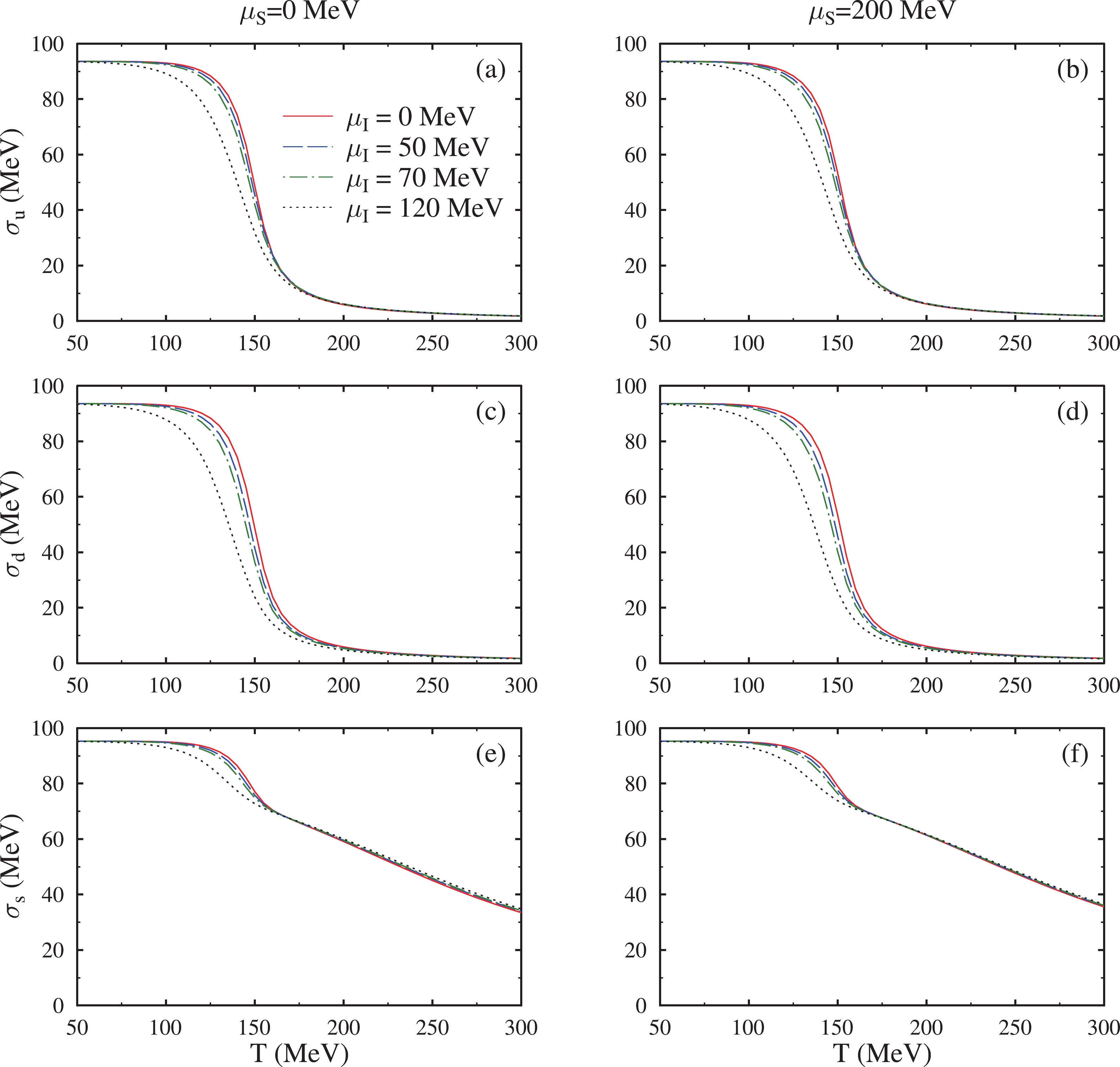
Figure 3. (color online) The quark condensates
$ \sigma_u $ ,$ \sigma_d $ , and$ \sigma_s $ as a function of temperature, T, for isospin chemical potential ($ \mu_I $ ) = 0, 50, 70, and 120 MeV, strangeness chemical potential,$ \mu_S $ = 0 and 200 MeV, and baryonic chemical potential fixed at$ \mu_B $ = 400 MeV (for v = 0.3).
Figure 4. (color online) The Polyakov loop variables, Φ and
$ \bar\Phi $ , as a function of temperature, T, for isospin chemical potential,$ \mu_I $ = 0, 50, 70 and 120 MeV, strangeness chemical potential,$ \mu_S $ = 0 and 200 MeV, and baryonic chemical potential fixed at$ \mu_B $ = 400 MeV(for v = 0.3)The quark condensate value became smaller with increasing temperature and increasing isospin chemical potential. The behavior of all quark condensates tended to be similar for higher values of temperature at different values of isospin chemical potential. The effect of changing value of isospin chemical potential was more evident in the case of light quarks. Up and down quarks showed similar trends at zero value of baryonic chemical potential, whereas at non zero
$ \mu_B $ , the, there was a slight difference in value at low temperature due to isospin asymmetric matter. With increase in isospin chemical potential, the difference between values of up and down quarks appeared to be more notable. For a given value of temperature, due to increase in strangeness chemical potential, the pseudo critical temperature was shifted to higher values.As seen in Fig. 4, at zero value of baryonic chemical potential, the results were the same for both the Polyakov loop variables. The value of Φ and
$ \bar{\Phi} $ increased with increase in temperature. The value of these fields appeared to be nearly zero at low temperature, indicating the confinement. The increase in value of isospin chemical potential increased the value of fields, and hence, a decrease in deconfinement temperature. At non zero value of$ \mu_B $ , Φ had low values until T ≈ 140 MeV, and then increased abruptly and became almost constant, showing the change from a confined to deconfined state. On other hand,$ \bar{\Phi} $ indicated a quite rapid increase in values at comparatively lower temperature. For non-zero values of strangeness chemical potential,$ \mu_S $ had significantly less effect on the distributions of Φ and$ \bar{\Phi} $ . -
In Sec. III.B, we compare the results from the two models described in the earlier sections. In Fig. 5 we plotted the effective quark masses,
$ m_{u}^{*} $ ,$ m_{d}^{*} $ , and$ m_{s}^{*} $ , as a function of temperature, T, for baryonic chemical potential,$ \mu_B $ = 400 MeV, and strangeness chemical potential,$ \mu_S $ = 200 MeV, with isospin chemical potential fixed at 120 MeV in both models. The constituent quark masses depended on the Yukawa coupling constant, g, which we fixed at g = 6.5, and values of quark condensates for the PQM model. On the other hand, in the PCQMF model, these depended on the non-strange scalar field, σ, strange scalar meson field, ζ, scalar isovector meson field, δ, and coupling constants,$ g_{\sigma i} $ ,$ g_{\zeta i} $ , and$ g_{\delta i} $ , representing the strength of interactions between different scalar fields and quarks. Hence the trend of quark masses was similar to that of quark condensates as a function of temperature. The value of constituent quark masses in vacuum was considered as$ m_{u}^{*} $ =$ m_{d}^{*} $ = 302 MeV and$ m_{s}^{*} $ = 437 MeV in the PQM model, and$ m_{u}^{*} $ =$ m_{d}^{*} $ = 313 MeV and$ m_{s}^{*} $ = 490 MeV in the PCQMF model. As was evident in both models, effective quark masses decreased with increased temperature. This was due to the fact that with rising temperature, the system evolved from a confined hadronic state to a deconfined quark-gluon plasma phase. We observed in plots of light quark condensates that with the increase in isospin chemical potential there was mass splitting between masses of up and down quarks. The change in value of mass was less eminent in strange quarks with changing isospin chemical potential. Due to differences in types of interactions explained and included by these two models, there was a slight difference in plots of masses, although the overall behaviour was quite similar in both models.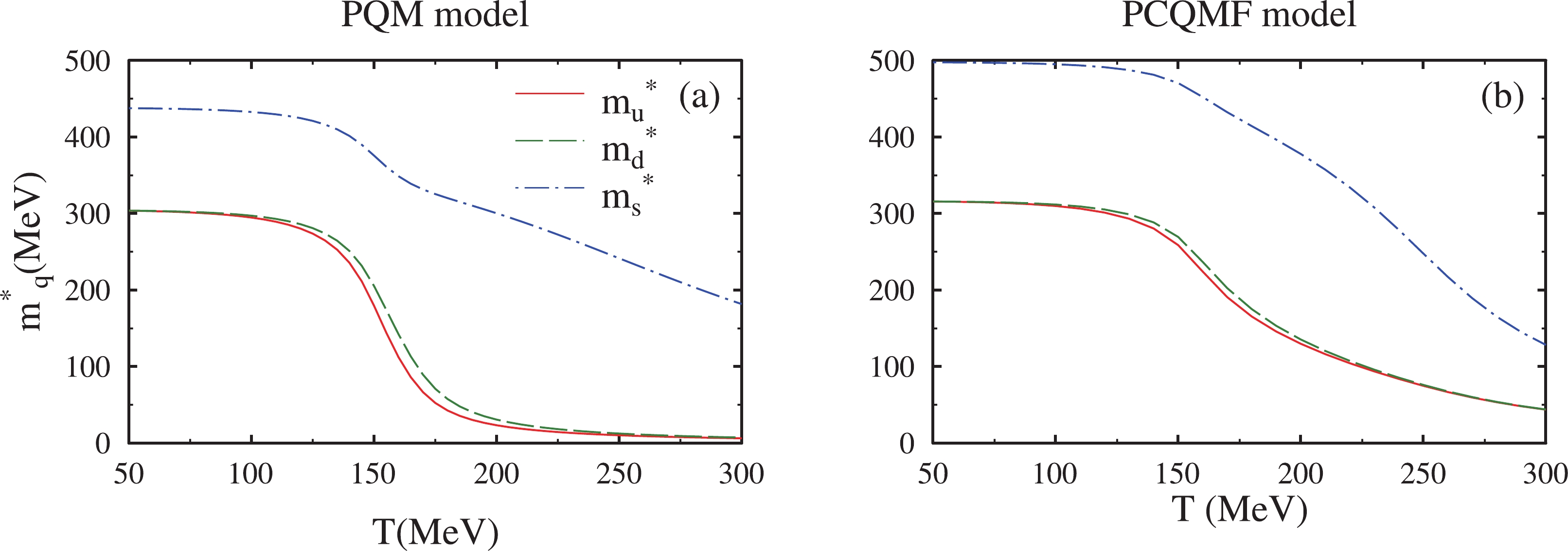
Figure 5. (color online) The effective quark masses,
$ m_{u}^{*} $ ,$ m_{d}^{*} $ and$ m_{s}^{*} $ , as a function of temperature, T, for baryonic chemical potential,$ \mu_B $ = 400 MeV, isospin chemical potential,$ \mu_I $ = 120 MeV, and strangeness chemical potential,$ \mu_S $ = 200 MeV, for the PQM model (a) and PCQMF model (b).The pressure and energy density calculated using the thermodynamic chemical potential was used to calculate the quantity (ϵ-3p)/
$ T^4 $ , which attributes to a trace anomaly property of the QCD. In Figure 6, we show the temperature dependence of$ p/T^4 $ , s/$ T^3 $ , ϵ/$ T^4 $ , and$ (\epsilon-3p)/T^4 $ with isospin chemical potential fixed at 120 MeV and baryonic chemical potential,$ \mu_B $ = 400 MeV, at strangeness chemical potential,$ \mu_S $ = 200 MeV, for the three-flavor quark matter in the PQM model and PCQMF model. These thermodynamic quantities have been studied in different theoretical models [80-83]. The value of the Stefan Boltzmann (SB) limit also changed with the change in number of quark flavors [84]. We showed that the value of these quantities increased with the shift from a two- to three-flavored system. The sudden change in these quantities represented the phase change from confinement of quarks to deconfinement at higher temperature values. From all plots, clearly, as the value of baryonic chemical potential increased, the phase change happened at lower temperatures. These thermodynamic variables were an important aspect to study the QCD phase structure.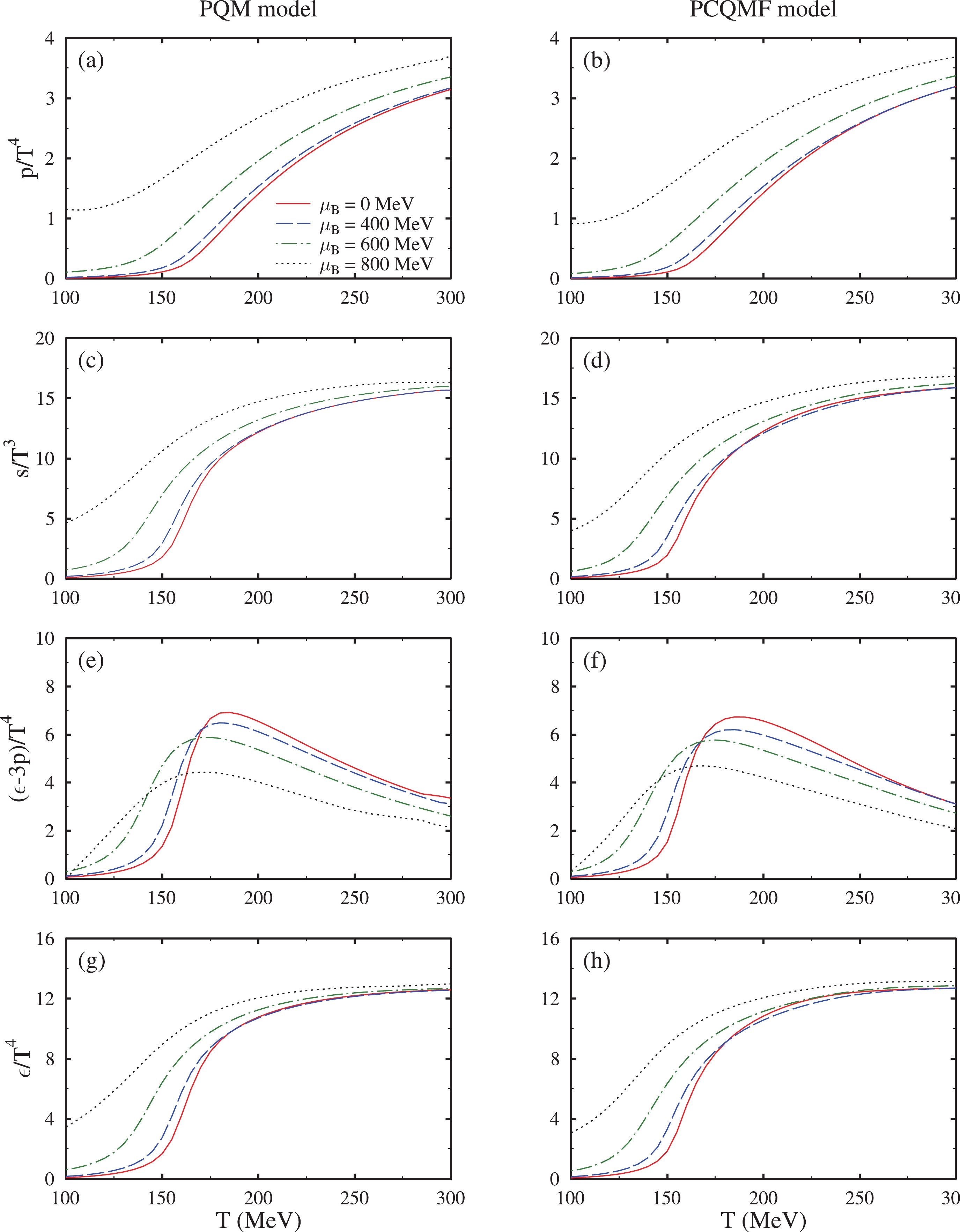
Figure 6. (color online) The pressure density, p, entropy density, s, trace anamoly, (ϵ-3P)/(
$ T^4 $ ), and energy density, ϵ, as a function of temperature, T, for isospin chemical potential,$ \mu_I $ = 70 MeV, baryonic chemical potential,$ \mu_B $ = 0, 400, 600, and 800 MeV, and strangeness chemical potential,$ \mu_S $ , fixed at 200 MeV for the PQM and PCQMF models.In Fig. 7, we plotted the (
$ T-\mu_q $ ) phase diagram of quark matter from the PQM model with different values of vector coupling ratio, v = 0, 0.5, and 1, at zero value of isospin chemical potential,$ \mu_I $ (left panel). On the right panel is the phase diagram for various isospin chemical potentials,$ \mu_I $ = 0, 50, and 70 MeV, and zero value of vector coupling ratio, v. At zero value of isospin chemical potential and vector coupling ratio, the critical-point (CP) was at T = 82 MeV and$ \mu_q $ = 285 MeV. The value of the critical-point was determined by plotting the susceptibilities of order parameters at varying values of quark chemical potential and temperature. At$ \mu_q = \mu_{q(\rm CP)} $ , the value of susceptibilities became infinite. The crossover region values were calculated by investigating the variation of quark condensate derivatives and Polyakov-loop variables at different temperatures and quark chemical potentials. At the CP, the first-order phase transition changed to crossover. For v = 0.5 and zero$ \mu_I $ , the critical-temperature was at 72 MeV, and quark chemical potential,$ \mu_{q(\rm CP)} $ = 290 MeV, and for v = 1,$ T_{\rm CP} $ = 55 MeV and$ \mu_{q(\rm CP)} $ = 310 MeV. With increased vector-coupling interaction ratio, the CP shifted to lower temperature and higher quark chemical potential. The similar effect of vector interactions on the phase diagram have been discussed in [47, 85]. The value of deconfinement temperature was calculated by plotting the derivatives of the Polyakov-loop parameters. The peak value of$ {\rm d}\Phi/{{\rm d}T} $ and$ {\rm d}\bar\Phi/{{\rm d}T} $ at varying values of quark chemical potential,$ \mu_q $ , and temperature gave the deconfinement transition temperature,$ T_C^d $ . For vector-interaction ratio, v = 0, and$ \mu_I $ = 50 MeV, the values were = 50 MeV, the values were$ T_{\rm CP} $ = 69 MeV and$ \mu_{q(\rm CP)} $ = 275 MeV. The critical point was ($ T_{\rm CP} $ ,$ \mu_{q(\rm CP)} $ ) = (55, 258) MeV for$ \mu_I $ = 70 MeV at zero value of vector-interaction ratio. From Fig. 7 (b), clearly, with increased isospin chemical potential, the critical-point moved to lower values of temperature and quark chemical potential. This behavior of critical-temperature and critical value of quark chemical potential is analogous to one discussed in [77, 86] for the PNJL model and PCQMF model. The phase transition line was, thus, modified due to change in the isospin chemical potential and vector-coupling ratio.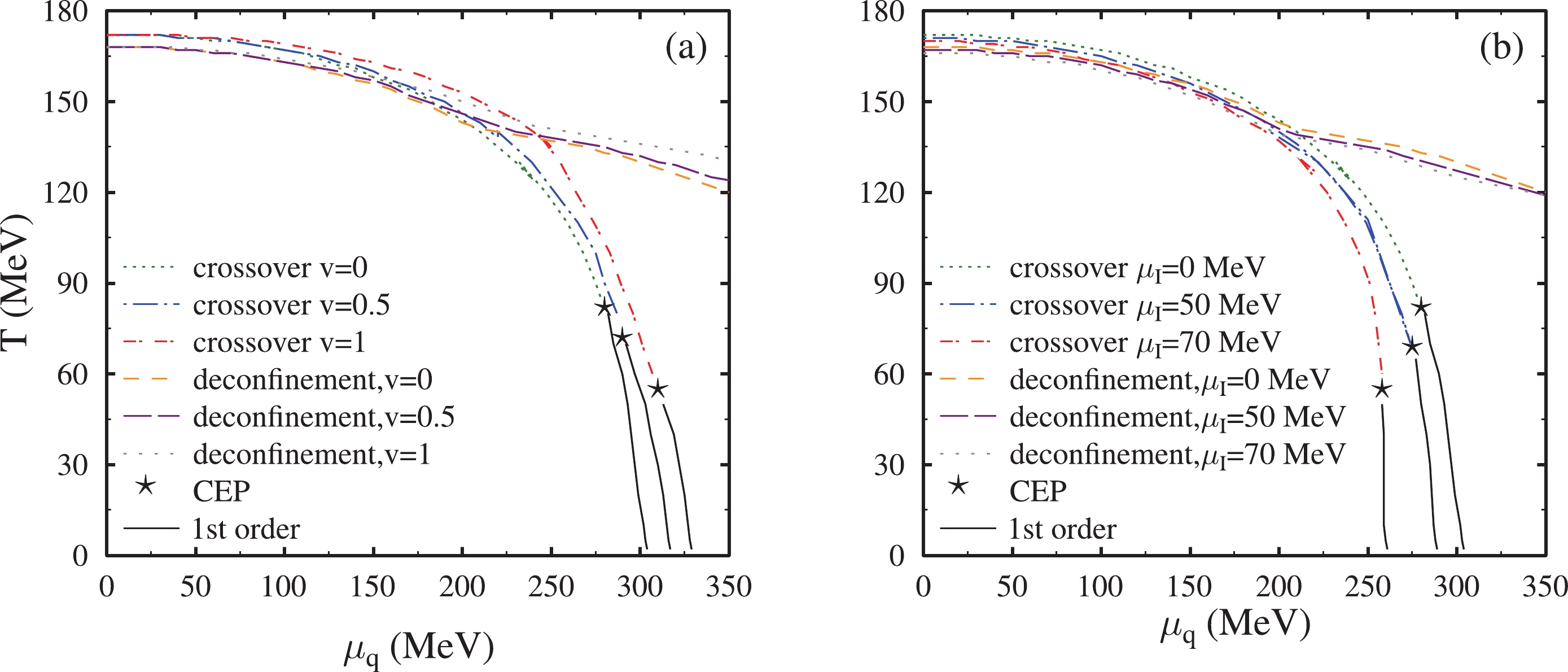
Figure 7. (color online) The
$ T-\mu_q $ phase diagram of quark matter from the PQM model with different values of vector coupling ratio, v = 0, 0.5, and 1, at zero value of isospin chemical potential,$ \mu_I $ (left panel). Phase diagram for various isospin chemical potentials,$ \mu_I $ = 0, 50, and 70 MeV, and zero value of vector coupling ratio, v (right panel). -
In this section, we discuss the results for susceptibilities of conserved charges in both the PQM and PCQMF models. At lower values of temperature, the quark condensates had very large values, and thus, corresponding quark masses were quite high. Due to which, the values of fluctuations of conserved quantities was relatively low. On the other hand, in the crossover regime, as a result of deconfinement, the quarks had very low mass. Hence the susceptibilities were enhanced as we approached in the vicinity of the transition temperature. Fluctuation of conserved charges was an important observable in order to study the phase transition and have been studied extensively in the Lattice QCD [87–91]. These observables provided us the direct signal of the critical-end point and helped in studying chiral symmetry restoration. For a medium in equilibrium, baryon number fluctuations is considered as a clear indication of a CEP. The non-monotonic dependence of fluctuations of these conserved quantities on collision energy in heavy-ion collision experiments verified the existence of a QCD critical-point [92]. The behavior of cumulants and susceptibilities of conserved charges have been investigated both experimentally and theoretically [70, 90, 93, 94].
In Fig. 8, we plotted the variation of second order,
$ \chi_{2}^B $ , and fourth order baryon number susceptibility,$ \chi_{4}^B $ , as a function of temperature for zero and low values of quark chemical potentials in the PQM and PCQMF models. The susceptibilities were plotted for vector-interaction coupling constant,$ g_v $ = 10.92 for the logarithmic form of the Polyakov-loop potential and$ g_v $ = 1.95 for the polynomial form of the Polyakov-loop potential. The theoretical results were compared to the lattice data from Bazavov, et al. [95, 96]. The second order susceptibilities rose monotonically with increased temperature, with fluctuations quite smaller at low temperatures and intensifying with change in relevant degrees of freedom. At zero value of quark chemical potential, there was a smooth rise in value of the second order baryon susceptibility in both models. The sharp increase in values of baryonic susceptibilities was due to the transformation from confined to deconfined quark states. A small kink was observed at a finite value of quark chemical potential near the transition temperature. A peaked behavior has previously been observed for second order baryon number susceptibility at higher values of chemical potential in vicinity of transition temperature [40]. A maximum height was attained by fourth order susceptibility at varying values of chemical potential. For finite values of quark chemical potential, the fluctuations were more heightened near the transition point, which was quite evident from the plots of second order baryon number susceptibility and fourth order baryon number susceptibility. The ratio of fourth order and second order susceptibility was determined as a key observable to define the position of the CEP due to its sensitivity for both deconfinement and chiral transitions [97, 98]. At low temperatures and vanishing quark chemical potential, the value of ($ \chi_{4}^B $ /$ \chi_{2}^B $ ) ≈ 1. However, at significantly high temperatures, ($ \chi_{4}^B $ /$ \chi_{2}^B $ ) ≈ 0.1, signifying the ideal gas behavior with quarks and gluons as degrees of freedom.
Figure 8. (color online) The second order baryon number susceptibility (
$ \chi_{2}^B $ ) and fourth order baryon number susceptibility ($ \chi_{4}^B $ ) as a function of temperature at$ {\mu}/{T} $ = 0, 0.2, and 0.4 for the PQM and PCQMF models. Values were calculated for$ g_v $ = 1.95 for polynomial Polyakov-loop and$ g_v $ = 10.92 for the logarithmic form of the Polyakov-loop potential and were compared with lattice data.In Fig. 9, we plotted the variation of skewness (
$ \chi_{3}^B $ /$ \chi_{2}^B $ ) and kurtosis ($ \chi_{4}^B $ /$ \chi_{2}^B $ ) of baryon number as a function of temperature at$ {\mu_q}/{T} $ = 0 and 0.4 for the PQM and PCQMF models. The main feature of these quantities was that they showed an abrupt change near the transition temperature region. The odd terms vanished in the Taylor series expansion due to charge-parity symmetry, and therefore, calculating the skewness at zero value of quark chemical potential was impossible. For both kurtosis and skewness, there was a sudden decrease in the value near the transition temperature due to change in phase from confined to deconfined. As the value of quark chemical potential was considered finite, these observables became more sensitive to the change in temperature and began to approach negative values. This shift of fourth order susceptibility, and hence kurtosis to negative values, can be attributed to the non-Gaussian behavior of the quark number distribution function after the phase transition [99].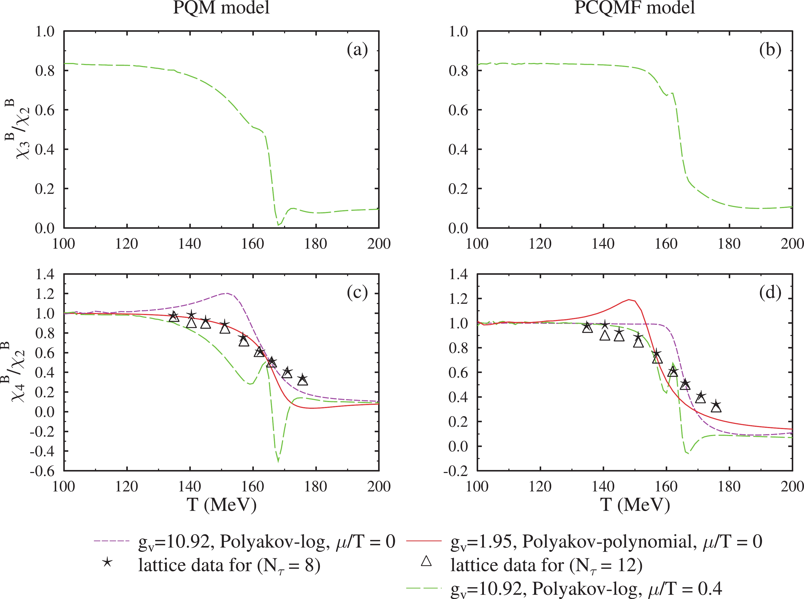
Figure 9. (color online) The skewness
$ \chi_{3}^B $ /$ \chi_{2}^B $ and kurtosis$ \chi_{4}^B $ /$ \chi_{2}^B $ of baryon number as a function of temperature at$ {\mu}/{T} $ = 0 and 0.4 for the PQM and PCQMF models. Values were calculated for$ g_v $ = 1.95 for the polynomial Polyakov-loop and$ g_v $ = 10.92 for the logarithmic form of the Polyakov-loop potential and were compared with lattice data.Figure 10 displays the change in sixth order and eighth order baryon number susceptibilities as a function of temperature in the PQM and PCQMF models. Contrary to variation of fourth order susceptibility exhibiting a peak at the transition region,
$ \chi_{6}^{B} $ and$ \chi_{8}^{B} $ only had positive and negative oscillating values in the transition region. A sudden fluctuation in the vicinity of the critical-point provided clear signature of transformation from one phase to another. The values for both models were slightly different. The results for the PCQMF model were more in agreement with those presented at zero quark chemical potential within the Polyakov extended NJL model [45].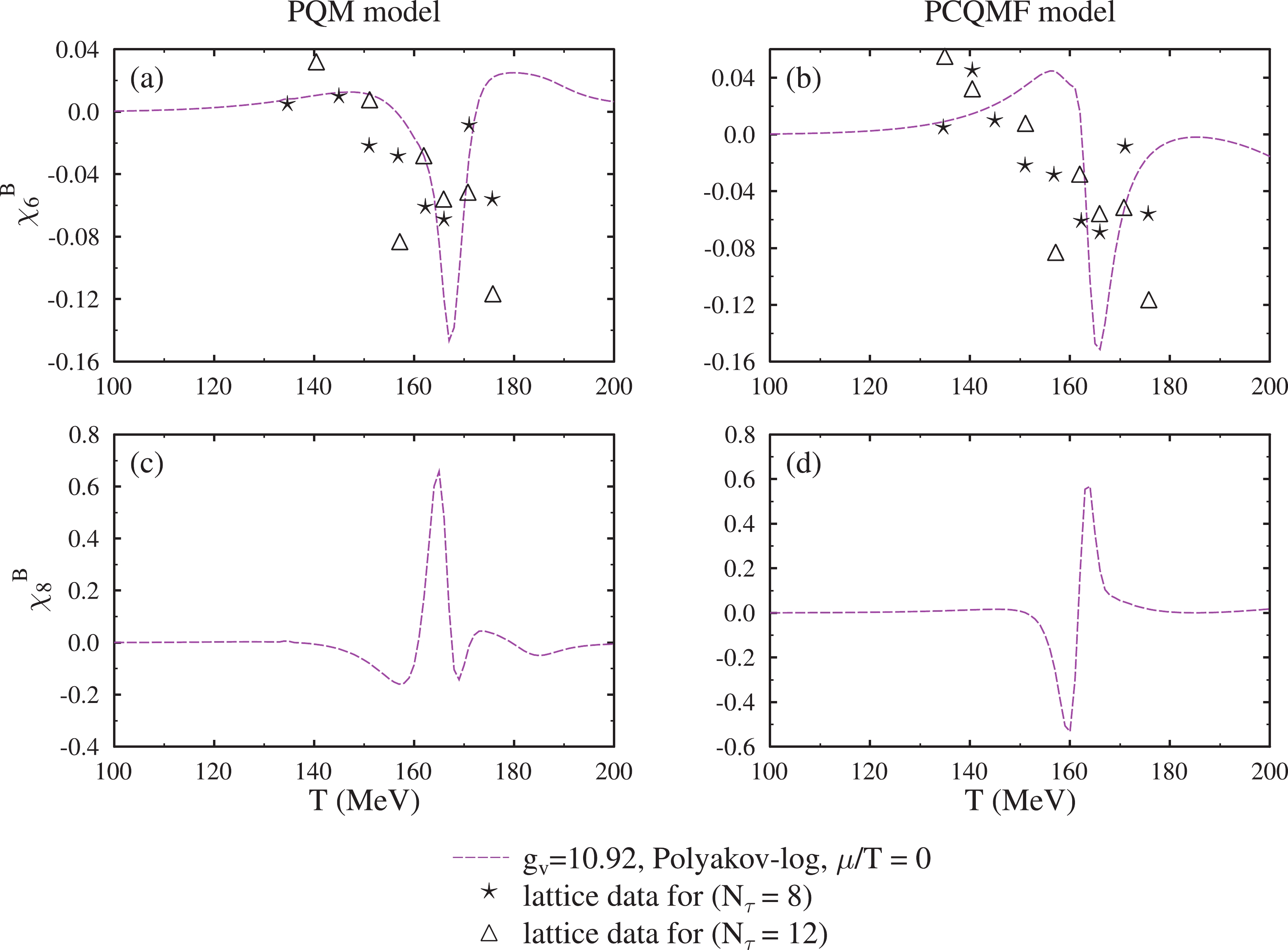
Figure 10. (color online) The sixth order (
$ \chi_{6}^{B} $ ) and eighth order ($ \chi_{8}^{B} $ ) baryon number susceptibility as a function of temperature in the PQM and PCQMF models at zero quark chemical potential. Values were calculated for$ g_v $ = 10.92 for the logarithmic form of the Polyakov-loop potential and were compared with lattice data.In the confined phase with hadronic degrees of freedom, strangeness was mainly contributed by strange mesons, like kaons. Due to the large masses of hadrons in this regime, the production of strange hadrons was highly suppressed [100, 101]. Contrarily, in the deconfined quark-gluon plasma phase, the total strangeness was carried by strange quarks having low mass. As a result of this, the strange number fluctuations should have a maximum value in this phase. Hence, this might serve as an important quantity signifying deconfinement transition [102, 103]. In Fig. 11 and Fig. 12, we plotted the variation of strangeness number susceptibility as a function of temperature. The second order susceptibility,
$ \chi_{2}^{S} $ , fourth order susceptibility,$ \chi_{4}^{S} $ , sixth order susceptibility,$ \chi_{6}^{S} $ , and ratio,$ \chi_{4}^{S} $ /$ \chi_{2}^{S} $ , were shown. The trend of$ \chi_{2}^{S} $ wa was similar to that of$ \chi_{2}^{B} $ , which was a monotonic behavior. But,$ \chi_{4}^{S} $ ,$ \chi_{6}^{S} $ , and ratio$ \chi_{4}^{S} $ /$ \chi_{2}^{S} $ showed a sudden increase in value, signalling the deconfinement at about ≈ 165 MeV. The trend of these observables was almost similar in both the models. The peaked value of susceptibilities for strangeness number was not only due to change in phase from hadrons to quarks and gluons, but also due to the change in effective masses of strange-hadrons. Thus, understanding whether the chiral and deconfinement does happen at the same temperature or not is another important parameter. The change of these variables can give a clear understanding of chiral restoration temperature as well as deconfinement.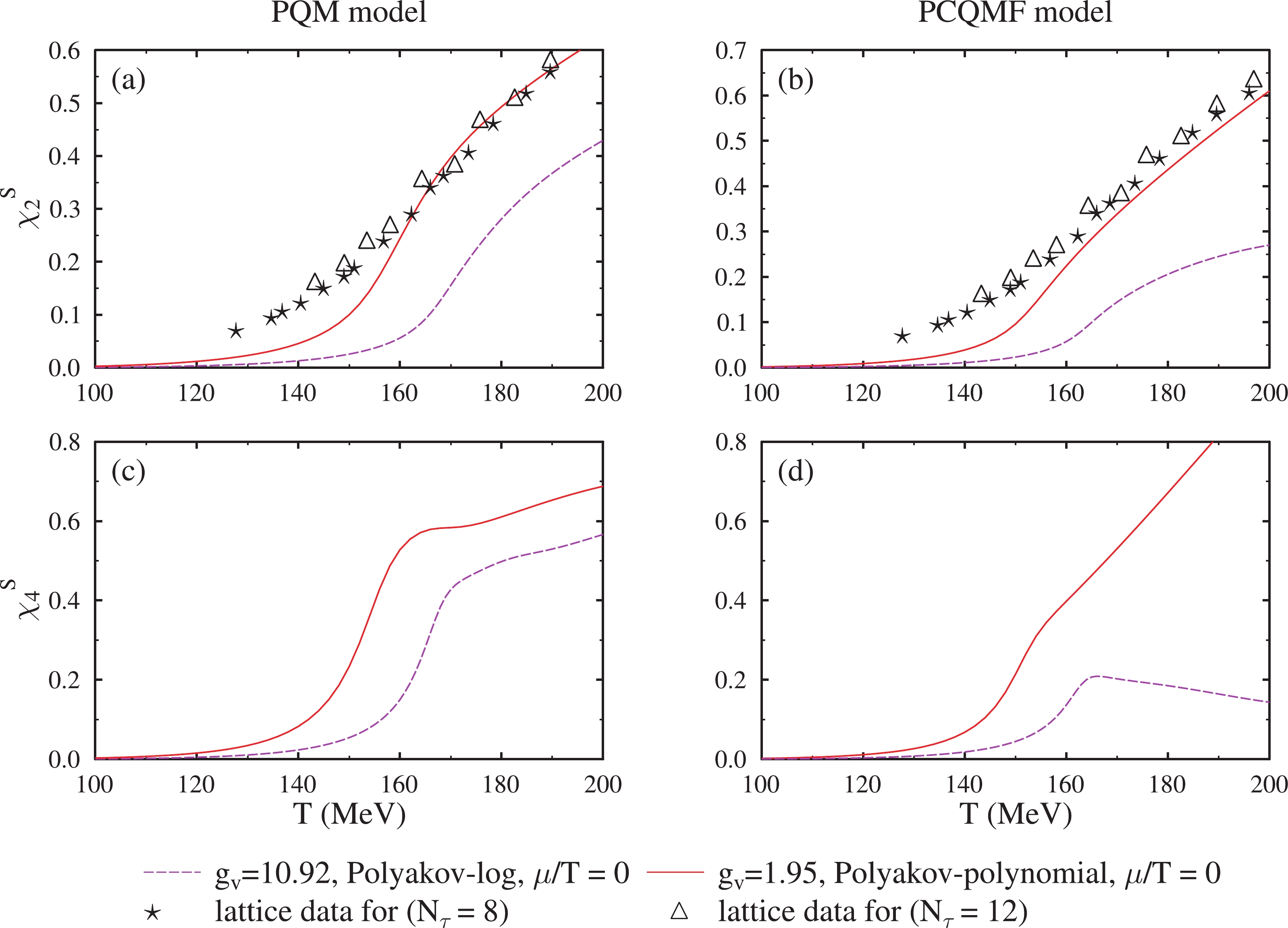
Figure 11. (color online) The second order susceptibility,
$ \chi_{2}^{S} $ , and fourth order susceptibility,$ \chi_{4}^{S} $ , plotted as a function of temperature for both the PQM amd PCQMF models at zero values of chemical potential. Values were calculated for$ g_v $ = 1.95 for polynomial Polyakov-loop and$ g_v $ = 10.92 for the logarithmic form of the Polyakov-loop potential, which were compared with lattice data.
Figure 12. (color online) The sixth order susceptibility,
$ \chi_{6}^{S} $ , and ratio,$ \chi_{4}^{S} $ /$ \chi_{2}^{S} $ , plotted as a function of temperature for both the PQM amd PCQMF models at zero values of strangeness chemical potential. Values were calculated for$ g_v $ = 1.95 for the polynomial Polyakov-loop and$ g_v $ = 10.92 for the logarithmic form of the Polyakov-loop potential.Cheng, et al. reported [90] that only the hadrons with low-masses, like pions, have significant contribution to fluctuations of electric charge number. Variation of these conserved quantities have been studied at high, as well as low temperatures, and are observed to carry information about relevant degrees of freedom [98, 101]. Bazavov, et al. showed [104] that net electric charge fluctuations are expected to be much greater than baryon number fluctuations in the vicinity of freeze-out, and hence are one of the most important observables to study the phase-transition. In Fig. 13 and Fig. 14, we show the change of electric charge number susceptibility as a function of temperature. The second order susceptibility,
$ \chi_{2}^{Q} $ , fourth order susceptibility, ity,$ \chi_{4}^{Q} $ , sixth order susceptibility, lity,$ \chi_{6}^{Q} $ , and ratio, ratio,$ \chi_{4}^{Q} $ /$ \chi_{2}^{Q} $ , were plotted. The second order susceptibility of all conserved charges showed a smooth increase for vanishing chemical potential. But, a peaked curve was obtained for fourth order, as well as sixth order, susceptibility. This sudden change in the values signified the transition temperature. The results for electric charge number susceptibilities were almost similar in both models. These values for the susceptibilities are in good agreement with the results presented in Chatterjee and Mohan [50].
Figure 13. (color online) The second order susceptibility
$ \chi_{2}^{Q} $ and fourth order susceptibility$ \chi_{4}^{Q} $ are plotted as a function of temperature for both PQM amd PCQMF model at zero values of chemical potential. Values have been calculated for$ g_v $ = 1.95 for polynomial Polyakov-loop and$ g_v $ = 10.92 for logarithmic form of Polyakov-loop potential and have been compared with lattice data.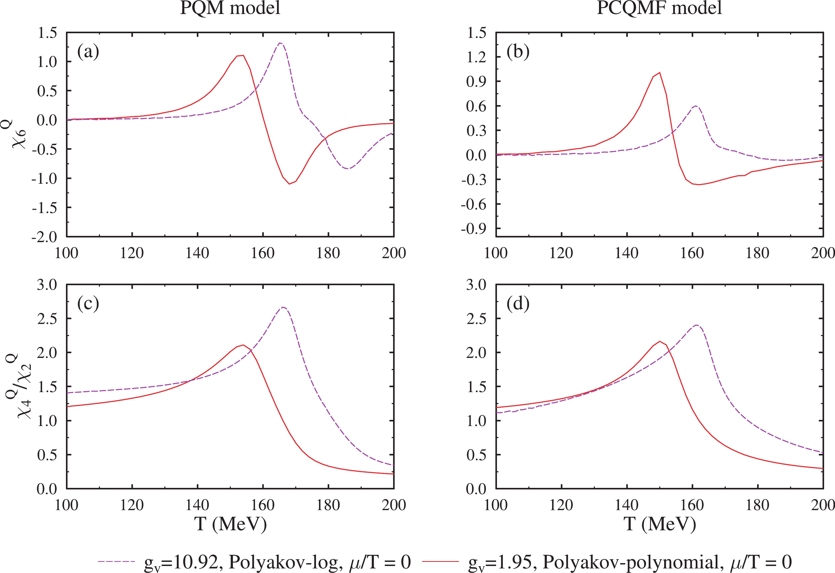
Figure 14. (color online) The sixth order susceptibility,
$ \chi_{6}^{Q} $ , and ratio,$ \chi_{4}^{Q} $ /$ \chi_{2}^{Q} $ , plotted as a function of temperature for both the PQM amd PCQMF models at zero values of chemical potential. Values were calculated for$ g_v $ = 1.95 for the polynomial Polyakov-loop and and$ g_v $ = 10.92 for the logarithmic form of the Polyakov-loop potential. -
We discussed the thermodynamic properties of the Polyakov loop extended quark-meson model and chiral quark mean-field model in asymmetric matter, including the vector and scalar interactions at finite density and temperature. The PQM model was modified by inclusion of vector fields and isospin chemical potential. The effects of isospin potential on the phase transition were investigated by studying the variation in order parameters with varying baryonic chemical potential in the PQM model. We found that with the increase in value of isospin chemical potential, first order transition changed to crossover. We comparatively analyzed the two theoretical models. Various thermodynamic variables, such as quark masses, pressure density, entropy density, and energy density, were plotted. Susceptibilities of conserved quantities, such as baryon number, strangeness number, and electric charge number, were inspected at different values of vector interaction coupling constant, as well as two forms of the Polyakov-loop potential. The results were compared to those of the lattice-QCD simulations. The transition temperatures for both the models were in the range of 160–165 MeV. In our future work, we will calculate the higher order cumulants and correlations of conserved charges at a finite value of chemical potential, adopting other differentiation methods, as well as the functional renormalization group approach, to include corrections beyond the mean-field approximation [105].
-
The authors sincerely acknowledge the support towards this work from the Ministry of Science and Human Resources (MHRD), Government of India via Institute fellowship under the National Institute of Technology Jalandhar.
-
Nonets of vector (
$ V_{\mu} $ ) and axial vector ($ A_{\mu} $ ) meson fields are given as$ \begin{aligned}[b] V^{\mu} =& \frac{1}{\sqrt{2}}\left(\begin{array}{ccc} \dfrac{\omega+\rho^{0}}{\sqrt{2}} & \rho^+ & K^{\star+} \\ \rho^- & \dfrac{\omega-\rho^{0}}{\sqrt{2}} & K^{\star 0} \\ K^{\star-} & K^{\star 0} & \phi \end{array}\right)^{\mu}\; \\A^{\mu} =& \frac{1}{\sqrt{2}}\left(\begin{array}{ccc} \dfrac{f_{1 }+a_{1}^{0}}{\sqrt{2}} & a_{1}^+ & K_{1}^+ \\ {a_{1}^-} & \dfrac{f_{1 }-a_{1}^{0}}{\sqrt{2}} & K_{1}^{0} \\ K_{1}^- & \bar{K}_{1}^{0} & f_{1\phi} \end{array}\right)^{\mu} \end{aligned} \tag{A1} $

Coupled equations for the PQM model are
$ \begin{aligned}[b] \frac{\partial \Omega}{\partial \sigma_u} =& \frac{\lambda_{1}}{4}\left[\sigma_u\left(\sigma_u^{2} + \sigma_d^{2}\right)+2 \sigma_u \sigma_s^{2}\right]\\&+\frac{\lambda_{2}}{4}\sigma_u^{3} -\frac{c}{2 \sqrt{2}}\sigma_d \sigma_s+ \frac{m^{2}}{2} \sigma_u-\frac{h_{u d}}{2}\\&+\frac{g}{2}\rho_{su} -\frac{N_{c} g m_{u}^{3} }{16\pi^{2}} \left[4 \log \frac{m_{u}}{\lambda}+1\right], \end{aligned}\tag{A2} $

$ \begin{aligned}[b] \frac{\partial \Omega}{\partial \sigma_d} =& \frac{\lambda_{1}}{4}\left[\sigma_d\left(\sigma_u^{2} + \sigma_d^{2}\right)+2 \sigma_d \sigma_s^{2}\right]\\&+\frac{\lambda_{2}}{4}\sigma_d^{3} -\frac{c}{2 \sqrt{2}}\sigma_u \sigma_s+ \frac{m^{2}}{2} \sigma_d-\frac{h_{u d}}{2}\\&+\frac{g}{2}\rho_{sd} -\frac{N_{c}g m_{d}^{3} }{16\pi^{2}} \left[4 \log \frac{m_{d}}{\lambda}+1\right], \end{aligned}\tag{A3} $

$ \begin{aligned}[b] \frac{\partial \Omega}{\partial \sigma_s} =& \frac{\lambda_{1}}{4}\left[4\sigma_s^{3}+2 \sigma_s\left(\sigma_u^{2} + \sigma_d^{2}\right)\right]\\&+\lambda_{2}\sigma_s^{3} -\frac{c}{2 \sqrt{2}}\sigma_u \sigma_d+ m^{2} \sigma_s-h_s\\&+\frac{g}{\sqrt{2}}\rho_{ss} -\frac{N_{c} g m_{s}^{3}}{8\sqrt{2}\pi^{2}} \left[4 \log \frac{m_{s}}{\lambda}+1\right], \end{aligned}\tag{A4} $

$ \begin{align} \frac{\partial \Omega}{\partial \omega} = -m_{\omega}^2\omega + \sum\limits_{i = u,d,s} g_{\omega i} \rho_{vi}, \end{align}\tag{A5} $

$ \begin{equation} \frac{\partial \Omega}{\partial \rho} = -m_{\rho}^2\rho + \sum\limits_{i = u,d,s} g_{\rho i} \rho_{vi},\;\; \end{equation} \tag{A6} $

$ \begin{equation} \frac{\partial \Omega}{\partial \phi} = -m_{\phi}^2\phi + \sum\limits_{i = u,d,s} g_{\phi i} \rho_{vi}. \end{equation}\tag{A7} $

In the above equations,
$ g_{\omega i} $ ,$ g_{\phi i} $ , and$ g_{\rho i} $ give the coupling strength of quarks and vector meson fields interactions. The equations for Φ and$ \bar \Phi $ are the same for the models due to consideration of the same form of the Polyakov-loop. Vector density is represented as$ \rho_{vi} $ , and$ \rho_{si} $ is the scalar density; these are defined as$ \begin{eqnarray} \rho_{vi} = \gamma_{i}N_c\int\frac{{\rm d}^{3}k}{(2\pi)^{3}} \Big(f_i(k)-\bar{f}_i(k) \Big), \end{eqnarray}\tag{A8} $

and
$ \begin{eqnarray} \rho_{si} = \gamma_{i}N_c\int\frac{{\rm d}^{3}k}{(2\pi)^{3}} \frac{m_{i}^{*}}{E^{\ast}_i(k)} \Big(f_i(k)+\bar{f}_i(k) \Big), \end{eqnarray}\tag{A9} $

respectively, where
$ f_i(k) $ and$ \bar{f}_i(k) $ represent the Fermi distribution functions at finite temperature for quarks and anti-quarks, and are defined as$ \begin{equation} f_{i}(k) = \frac{\Phi {\rm e}^{-(E_i^*(k)-{\nu_i}^{*})/k_BT}+2\bar{\Phi} {\rm e}^{-2(E_i^*(k)-{\nu_i}^{*})/k_BT}+{\rm e}^{-3(E_i^*(k)-{\nu_i}^{*})/k_BT}} {1+3\Phi {\rm e}^{-(E_i^*(k)-{\nu_i}^{*})/k_BT}+3\bar{\Phi} {\rm e}^{-2(E_i^*(k)-{\nu_i}^{*})/k_BT}+{\rm e}^{-3(E_i^*(k)-{\nu_i}^{*})/k_BT}} \; \end{equation} \tag{A10} $

$ \begin{equation} \bar{f}_{i}(k) = \frac{\bar{\Phi} {\rm e}^{-(E_i^*(k)+{\nu_i}^{*})/k_BT}+2{\Phi} {\rm e}^{-2(E_i^*(k)+{\nu_i}^{*})/k_BT}+{\rm e}^ {-3(E_i^*(k)+{\nu_i}^{*})/k_BT}}{1+3\bar{\Phi} {\rm e}^{-(E_i^*(k)+{\nu_i}^{*})/k_BT}+3{\Phi} {\rm e}^{-2(E_i^*(k)+{\nu_i}^{*})/k_BT}+{\rm e}^{-3(E_i^*(k)+{\nu_i}^{*})/k_BT}} . \end{equation} \tag{A11}$

This value is the same for both the models. By solving the coupled equations, we obtain the values of quark condensates and different fields at varying values of temperature and density.
The coupled equations for the PCQMF model are given as
$ \begin{aligned}[b] \frac{\partial \Omega}{\partial \sigma} =& k_{0}\chi^{2}\sigma-4k_{1}\left( \sigma^{2}+\zeta^{2} +\delta^{2}\right)\sigma-2k_{2}\left( \sigma^{3}+3\sigma\delta^{2}\right) \\&-2k_{3}\chi\sigma\zeta - \frac{d}{3} \chi^{4} \bigg (\frac{2\sigma}{\sigma^{2}-\delta^{2}}\bigg ) +\left( \frac{\chi}{\chi_{0}}\right) ^{2}m_{\pi}^{2}f_{\pi} \\&- \left(\frac{\chi}{\chi_0}\right)^2m_\omega\omega^2 \frac{\partial m_\omega}{\partial\sigma} \left(\frac{\chi}{\chi_0}\right)^2m_\rho\rho^2 \frac{\partial m_\rho}{\partial\sigma} -\sum\limits_{i = u,d} g_{\sigma i}\rho_{si} = 0 , \end{aligned}\tag{A12} $

$ \begin{aligned}[b] \frac{\partial \Omega}{\partial \zeta} =& k_{0}\chi^{2}\zeta-4k_{1}\left( \sigma^{2}+\zeta^{2}+\delta^{2}\right) \zeta-4k_{2}\zeta^{3}\\&-k_{3}\chi\left( \sigma^{2}-\delta^{2}\right)-\frac{d}{3}\frac{\chi^{4}}{{\zeta}} +\left(\frac{\chi}{\chi_{0}} \right) ^{2}\\&\times\left[ \sqrt{2}m_{K}^{2}f_{K}-\frac{1}{\sqrt{2}} m_{\pi}^{2}f_{\pi}\right] \\& -\left(\frac{\chi}{\chi_0}\right)^2m_\phi\phi^2 \frac{\partial m_\phi}{\partial\zeta} -\sum\limits_{i = s} g_{\zeta i}\rho_{si} = 0 , \end{aligned}\tag{A13} $

$ \begin{aligned}[b] \frac{\partial \Omega}{\partial \delta} =& k_{0}\chi^{2}\delta-4k_{1}\left( \sigma^{2}+\zeta^{2}+\delta^{2}\right) \delta-2k_{2}\left( \delta^{3}+3\sigma^{2}\delta\right)\\& +\mathrm{2k_{3}\chi\delta \zeta} + \frac{2}{3} d \chi^4 \left( \frac{\delta}{\sigma^{2}-\delta^{2}}\right) -\sum\limits_{i = u,d} g_{\delta i}\rho_{vi} = 0 , \end{aligned}\tag{A14} $

$ \begin{aligned}[b] \frac{\partial \Omega}{\partial \chi} = &\mathrm{k_{0}}\chi \left( \sigma^{2}+\zeta^{2}+\delta^{2}\right)-k_{3} \left( \sigma^{2}-\delta^{2}\right)\zeta + \chi^{3}\left[1 +{\rm{ln}}\left( \frac{\chi^{4}}{\chi_{0}^{4}}\right) \right] +(4k_{4}-d)\chi^{3} - \frac{4}{3} d \chi^{3} {\rm{ln}} \left ( \left (\frac{\left( \sigma^{2} -\delta^{2}\right) \zeta}{\sigma_{0}^{2}\zeta_{0}} \right ) \left (\frac{\chi}{{\chi_0}}\right)^3 \right ) \\&+ \frac{2\chi}{\chi_{0}^{2}}\left[ m_{\pi}^{2} f_{\pi}\sigma +\left(\sqrt{2}m_{K}^{2}f_{K}-\frac{1}{\sqrt{2}} m_{\pi}^{2}f_{\pi} \right) \zeta\right] - \frac{\chi}{{\chi^2}_0}({m_{\omega}}^2 \omega^2+{m_{\rho}}^2\rho^2) = 0, \end{aligned}\tag{A15} $

$ \frac{\partial \Omega}{\partial \omega} = \frac{\chi^2}{\chi_0^2}m_\omega^2\omega+4g_4\omega^3+ 12g_4\omega\rho^2-\sum\limits_{i = u,d}g_{\omega i}\rho_{vi} = 0, \tag{A16}$

$ \frac{\partial \Omega}{\partial \rho} = \frac{\chi^2}{\chi_0^2}m_\rho^2\rho+4g_4\rho^3+12g_4\omega^2\rho- \sum\limits_{i = u,d}g_{\rho i}\rho_{vi} = 0, \tag{A17} $

$ \frac{\partial \Omega}{\partial \phi} = \frac{\chi^2}{\chi_0^2}m_\phi^2\phi+8g_4\phi^3- \sum\limits_{i = s}g_{\phi i}\rho_{vi} = 0, \tag{A18} $

$ \begin{aligned}[b] \frac{\partial \Omega}{\partial \Phi} =& \bigg[\frac{-a(T)\bar{\Phi}}{2}-\frac{6b(T) (\bar{\Phi}-2{\Phi}^2+{\bar{\Phi}}^2\Phi) }{1-6\bar{\Phi}\Phi+4(\bar{\Phi}^3+\Phi^3)-3(\bar{\Phi}\Phi)^2}\bigg]T^4 \\&-\sum\limits_{i = u,d,s}\frac{2k_{\rm B}TN_{\rm C}}{(2\pi)^3} \int_0^\infty {\rm d}^3k \bigg[\frac{{\rm e}^{-(E_i^*(k)-{\nu_i}^{*})/k_{\rm B}T}}{(1+{\rm e}^{-3(E_i^*(k)-{\nu_i}^{*})/k_{\rm B}T}+3\Phi {\rm e}^{-(E_i^*(k)-{\nu_i}^{*})/k_{\rm B}T} +3\bar{\Phi}{\rm e}^{-2(E_i^*(k)-{\nu_i}^{*})/k_{\rm B}T})} \\& +\frac{{\rm e}^{-2(E_i^*(k)+{\nu_i}^{*})/k_{\rm B}T}}{(1+{\rm e}^{-3(E_i^*(k)+{\nu_i}^{*})/k_{\rm B}T} +3\bar{\Phi} {\rm e}^{-(E_i^*(k)+{\nu_i}^{*})/k_{\rm B}T}+3\Phi {\rm e}^{-2(E_i^*(k)+{\nu_i}^{*})/k_{\rm B}T})}\bigg] = 0, \end{aligned}\tag{A19} $

and
$ \begin{aligned}[b] \frac{\partial \Omega}{\partial \bar{\Phi}} =& \bigg[\frac{-a(T)\Phi}{2}-\frac{6b(T) (\Phi-2{\bar{\Phi}}^2+{\Phi}^2\bar{\Phi}) }{{1-6\bar{\Phi}\Phi+4(\bar{\Phi}^3+\Phi^3)-3(\bar{\Phi}\Phi)^2}}\bigg]T^4\\& -\sum\limits_{i = u,d,s}\frac{2k_{\rm B}TN_{\rm C}}{(2\pi)^3} \int_0^\infty {\rm d}^3k\ \bigg[\frac{{\rm e}^{-2(E_i^*(k)-{\nu_i}^{*})/k_{\rm B}T}}{1+{\rm e}^{-3(E_i^*(k)-{\nu_i}^{*})/k_{\rm B}T}+3\Phi {\rm e}^{-(E_i^*(k)-{\nu_i}^{*})/k_{\rm B}T} +3\bar{\Phi}{\rm e}^{-2(E_i^*(k)-{\nu_i}^{*})/k_{\rm B}T}} \\& +\frac{{\rm e}^{-(E_i^*(k)+{\nu_i}^{*})/k_{\rm B}T}}{1+{\rm e}^{-3(E_i^*(k)+{\nu_i}^{*})/k_{\rm B}T} +3\bar{\Phi} {\rm e}^{-(E_i^*(k)+{\nu_i}^{*})/k_{\rm B}T}+3\Phi {\rm e}^{-2(E_i^*(k)+{\nu_i}^{*})/k_{\rm B}T}}\bigg] = 0. \end{aligned} \tag{A20}$

Quark matter properties and fluctuations of conserved charges in (2+1)-flavored quark model
- Received Date: 2021-12-21
- Available Online: 2022-06-15
Abstract: In this study, the susceptibilities of conserved charges, baryon number, charge number, and strangeness number at zero and low values of chemical potential are presented. Taylor series expansion was used to obtain results for the three-flavor Polyakov quark meson (PQM) model and the Polyakov loop extended chiral quark mean-field (PCQMF) model. Mean-field approximation was used to study quark matter with the inclusion of the isospin chemical potential, as well as the vector interactions. The effects of isospin chemical potential and vector-interactions on phase diagrams were analyzed. A comparative analysis of the two models was completed. Fluctuations of the conserved charges were enhanced in the transition temperature regime and hence provided information about the critical end point (CEP). Susceptibilities of conserved quantities were calculated by using the Taylor series method. Enhancement of fluctuations in the transition temperature neighborhood provided a clear signature of a quantum chromodynamics (QCD) critical-point.


 DownLoad: