


 Abstract
 HTML
HTML Reference
 Related
 PDF
PDF


-
The Black Hole's apparent shape from a distant observer when illuminated by a source of light is referred to as a black hole shadow. When light emitting from the accretion passes through the vicinity of the black hole toward the observer, its trajectory will be deflected. The intensity of the light observed by the distant observer differs accordingly, leading to a dark interior and bright ring. When a shadow appears, the light, or photons, can orbit around this spherically symmetric black hole at a constant radius, which forms a bright ring called the photon sphere. Although such an orbit is unstable, it remains important from a physical perspective because it defines the boundary for a BH shadow between the capture and non-capture of a cross-section of light rays by the black hole. This boundary has played an important role in determining, for example, the optical appearance of a black hole with thin accretions [1]. Most of the light illuminating the black hole originates from the accretion around it, and the models of the accretion matter will influence the formation of the shadows. For a geometrically thin, optically thick accretion disk, it was determined that the mass of the disk would affect the shadow of a black hole; as the mass increases, the shadow becomes more prolate [2]. The edge of the shadow is also deduced to be independent of the inner radius at which the accreting gas stops radiating [3].
The Event Horizon Telescope (EHT) collaboration, which is now the world's biggest astronomy project, reported 1.3 mm Very Long Baseline Interferometry (VLBI) observations of the nucleus of the nearby galaxy M87, achieving angular resolution comparable to the expected size of the supermassive black hole [4–9]. It promotes the current theoretical study on black hole based on modern astronomical observation methods. This project also corroborates the direct observations of the black hole shadows. Furthermore, the shape of a shadow could be used to study gravity near the event horizon and determine whether the general relativity is consistent with the observations [10], which enables a direct probe of the General Relativity (GR) in the extreme environment.
The shadow of the Schwarzschild black hole was first discussed in [11]. Bardeen [12] soon studied the shadow cast by the Kerr black hole. The photon rings and lensing rings was studied with analytic calculations and numerical models [13]. Lensing by Kerr Black Holes has been investigated [14], and it was also studied the influence of quantum correction on black hole shadows [15]. Moreover, this method has been extended to the Asymmetric Thin-shell Wormhole (ATW) about its photon rings [16]. Multiple shadows of a single black hole have also been discussed [17,18], including the shadow of multiple black holes [19]. The black hole shadow in modified GR has also been investigated in [20–22]. The models of the black hole, considering the accretion that can modify the silhouette, are studied in [23–25]. Recently, this topic has been extended to many other black holes by various researchers [26–43].
We consider the black hole with dark energy, as the Standard Model of cosmology suggests that dark energy is dominant in our universe [44, 45] and its dynamic may affect the black hole [46] whose effect on spacetime is similar to the cosmological constant or vacuum energy [47]. Moreover, modern astronomical observers have deduced that the universe is in accelerating expansion [48–50], implying a state of negative pressure. In addition, the quintessence dark energy is one of the candidates for interpreting the negative pressure [51]. In this model, the state equation of the pressure is
$ p=\omega_q\rho _q $ , where$ \rho _q $ denotes the energy density and$ \omega_q $ represents the state parameter that satisfies$ -1<\omega_q<-1/3 $ [52–55]. The effect of an accelerated expanding universe on the shadow of a black hole is studied in [56]. It is also natural to study the effect of the quintessence dark energy [46], and the investigation can provide novel insights and impose restrictions on the quintessence model [57]. Shadows influenced by other dark energy models are studied in [58, 59].Theoretical developments propose that the basic unit of nature is one-dimensional strings, instead of point-like particles. Studying Einstein's equations with string clouds may be critical because relativistic strings can be employed to construct suitable models [60]. A cloud of strings as the source of a gravitational field was first considered by Latelier, who determined an exact solution of the Schwarzschild BH surrounded by a cloud of strings [61]. Later, the rotating BH with a cloud of strings was investigated [62, 63]. Then, the study of a cloud of strings was extended to modified theories of gravity such as Lovelock gravity [64, 65]. Recently, the exact solution of Schwarzschild black hole surrounded by a cloud of strings in Rastall gravity is obtained in [66].
In this study, we investigate the shadow and photon spheres of the black hole surrounded by a cloud of strings and quintessence with both static and infalling spherical accretions. The black hole thermodynamics combined effects of the string clouds and quintessence are considered in [67]. Afterwards, studies in this area were proposed for a charged AdS black hole [68], as well as Lovelock gravity [69]. Furthermore, we explore how the photons emissivity
$ j(\nu _e) $ affects the shadow of the black hole.This remainder of this paper is organized as follows. In Section II, we provide the metric of a black hole surrounded by quintessence and clouds of strings. Then, we derive the complete null geodesic equations for a photon moving around the static black hole. In addition, the range of parameters affected by string clouds is discussed. In Section III, we study the shadows and photon spheres with static spherical accretions of the static black hole. In Section IV, the black hole shadows and photon spheres with an infalling spherical accretion are investigated. In Section V, we discuss and conclude our results.
-
The metric of an uncharged static black hole surrounded by quintessence and clouds of strings is given by [67]
$ \begin{align} {\rm d}s^2=-f(r){\rm d}t^2+\frac{1}{f(r)}{\rm d}r^2+r^2({\rm d}\theta ^2+{\rm sin}^2\theta {\rm d}\phi ^2), \end{align} $

(1) with
$ \begin{align} f(r)=1-a-\frac{2M}{r}-\frac{\alpha }{r^{3\omega_q+1}}, \end{align} $

(2) where a is the constant affected by the cloud of strings, M is the mass of the black hole,
$ \omega_q $ is the state parameter of quintessence, and α is a constant related to the quintessence with density$ \rho_q $ as$ \begin{align} \rho_q=-\frac{\alpha}{2}\frac{3\omega_q }{r^{3(\omega_q+1)}}. \end{align} $

(3) The pressure of the quintessence dark energy p should be negative owing to the cosmic acceleration. The range of
$ \omega_q $ is$ -1 < \omega_q < -1/3 $ for$ p=\omega_q \rho_q $ [52–55], which triggers the emergence of event and cosmological horizons. In addition, the region between the two event horizons is called the outer communication domain, because any two observers in it can communicate with each other without being blocked [70, 71].Setting
$ f(r)=0 $ to obtain two roots, the smaller one is the radius of the event horizon$ r_h $ and the other is the cosmological horizon$ r_c $ . In general, it is not easy to get analytic solutions, but for$ \omega_q=-2/3 $ , the analytical solutions of$ f(r)=0 $ can be expressed as$ \begin{align} r_h & =\frac{1 - a + \sqrt{(1-a)^2 - 8 M \alpha}}{2\alpha}, \end{align} $

(4) $ \begin{align} r_c & =\frac{a - 1 + \sqrt{(1-a)^2 - 8 M \alpha}}{2\alpha}. \end{align} $

(5) The numerical values of
$ r_c $ ,$ r_h $ corresponding to other$ \omega_q $ are presented in Table 1.$ \omega_q $ 

−1/3 −0.4 −0.5 −0.6 −2/3 −0.7 −0.8 −0.9 −1 $ r_{ph} $ 

3.37079 3.3764 3.38524 3.39346 3.39746 3.39860 3.39602 3.37792 3.33333 $ b_{ph} $ 

5.37669 6.21753 6.27757 6.36711 6.45119 6.50322 6.71598 7.06308 7.66965 $ r_h $ 

2.04402 2.25165 2.25997 2.27085 2.27998 2.28525 2.30464 2.33145 2.37016 $ r_c $ 

− $ 5.9\times 10^9 $ 

8095.55 274.403 87.7200 57.6865 23.1518 12.5872 8.07703 Table 1. Data of
$ r_{ph} $ ,$ b_{ph} $ ,$ r_h $ and$ r_c $ for different$ \omega_q $ with$ M = 1 $ ,$ \alpha = 0.01 $ and$ a=0.1 $ .Then, we calculate the geodesic of photons to investigate the light deflection with the Euler-Lagrange equation. The Lagrangian takes the form
$ \begin{align} \mathcal{L} =\frac{1}{2}g_{\mu v}\dot{x}^{\mu}\dot{x}^{v}, \end{align} $

(6) where the dot represents the derivative to the affine parameter.
Owing to the spherical symmetry of metric, it is convenient to study the photon trajectories on the equatorial plane with the initial condition
$ \theta=\pi/2 $ and$ \dot{\theta}=0 $ . Combining Eqs. (1) and (6) with the Euler-Lagrange equation, we obtain the expressions of time, azimuth, and radial components for the four velocities. Because the metric does not explicitly depend on the time t and azimuthal angle ϕ, there are two corresponding conserved quantities E and L. Then, by redefining the affine parameter λ as$ \lambda/{\left\lvert L\right\rvert } $ and using the impact parameter$ b={\left\lvert L\right\rvert}/E $ [72], we obtain the following equations$ \begin{align} \dot{t} & =\frac{1}{bf(r)}, \end{align} $

(7) $ \begin{align} \dot{\phi} & =\pm \frac{1}{r^2}, \end{align} $

(8) $ \begin{align} \frac{1}{b^2} & =\dot{r}^2+\frac{1}{r^2}f(r) , \end{align} $

(9) where
$ + $ and$ - $ in Eq. (8) represent the counterclockwise and clockwise direction, respectively for the motion of photons. Moreover, Eq. (9) can be rewritten as$ \begin{align} \dot{r}^2+V(r)=\frac{1}{b^2}, \end{align} $

(10) where
$ V(r)=1/{r^2}f(r) $ is the effective potential. At the photon sphere, the photon trajectories satisfy$ \dot{r}=0 $ and$ \ddot{r}=0 $ , which implies that$ \begin{align} V(r)=\frac{1}{b^2}, \quad \ \ V'(r)=0. \end{align} $

(11) In general, for the radius of photon sphere
$ r_{ph} $ and corresponding impact parameter$ b_{ph} $ , it is difficult to obtain the analytic results. However, for$ \omega_q=-2/3 $ , they can be expressed as$ \begin{align} r_{ph} & =\frac{1-a-\beta}{\alpha}, \end{align} $

(12) $ \begin{align} b_{ph} & =\sqrt{-\frac{\left(\beta +a-1\right)^3}{\alpha ^2 \left(-a \left(\beta +a-2\right)+\beta +4 \alpha M-1\right)}}, \end{align} $

(13) where
$ \begin{align} \beta=\sqrt{(1-a)^2-6 \alpha M}. \end{align} $

(14) To obtain a realistic solution, there are restrictions
$ (1-a)^2\geqslant 6\alpha M $ between a and α with$ \omega_q=-2/3 $ . Similar numerical results can be obtained for other$ \omega_q $ .The data of
$ r_{ph} $ ,$ b_{ph} $ ,$ r_h $ , and$ r_c $ are presented in Table 1 with$ \alpha = 0.01 $ ,$ M=1 $ and$ a=0.1 $ . The$ b_{ph} $ ,$ r_h $ , and$ r_c $ are monotonic while$ r_{ph} $ is non-monotonic with the decrease in$ \omega_q $ . The event horizon radius$ r_c $ approaches the cosmological horizon radius$ r_h $ with the decrease in$ \omega_q $ , which leads to a narrower domain of the outer communication. It is worth noting that when$ \omega_q=-1/3 $ , the cosmological horizon radius$ r_c $ does not exist, which we denote with "-."The Eq. (10) demonstrates that the null geodesic depends on the impact parameter b and the effective potential
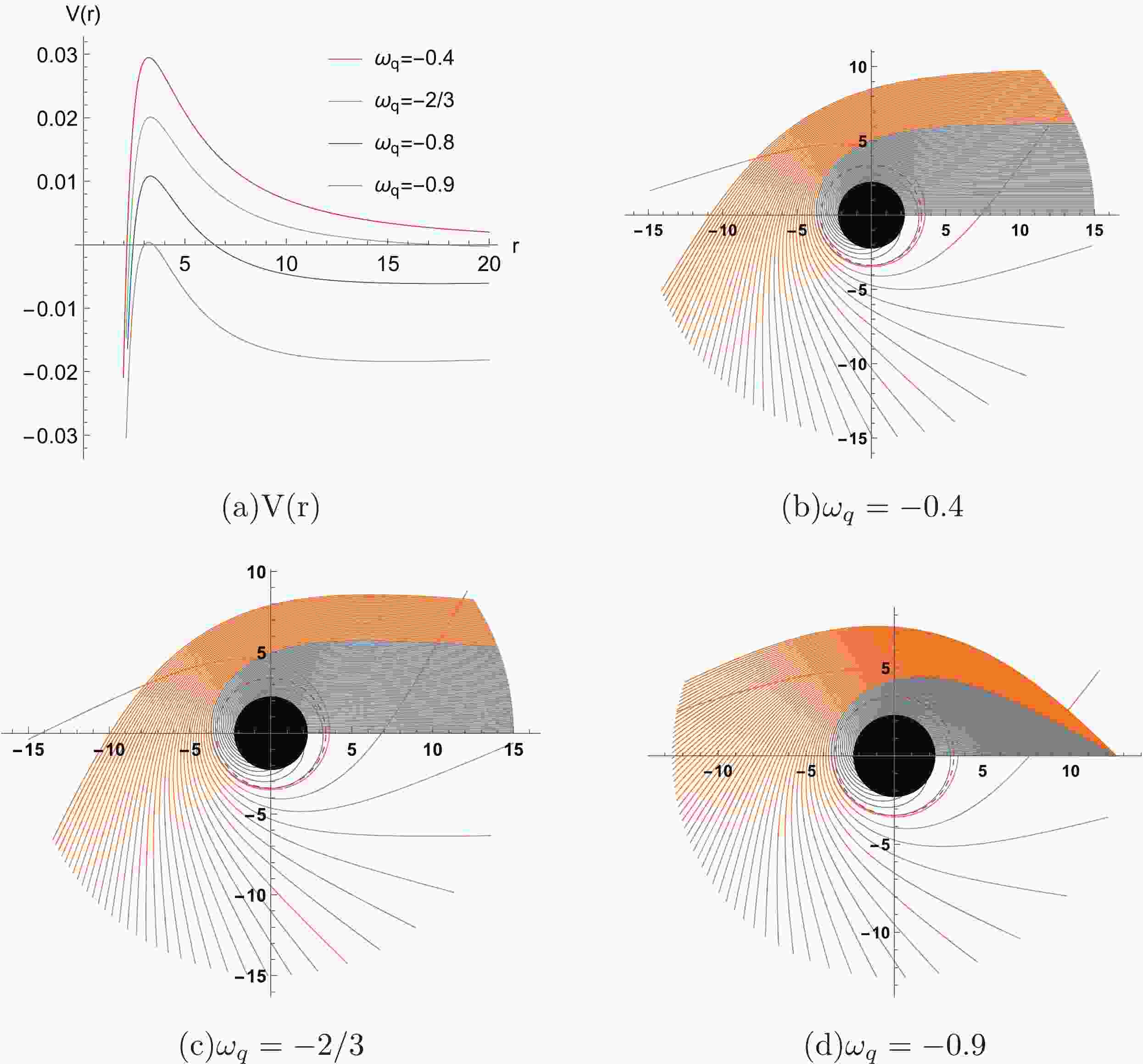
$ V(r) $ . The effective potential for different$ \omega_q $ is plotted in Fig. 1 (a). The effective potential vanishes at the event horizon, increases and reaches a maximum at the photon sphere, and finally vanishes at the cosmological horizon.
Figure 1. (color online) Effective potential
$ V(r) $ in Fig. 1 (a) and the trajectories of the photons in other images for different$ \omega_q $ with$ \alpha =0.01 $ and$ a=0.1 $ .The geodesics of photons can be plotted by the equation of motion. Combining Eqs. (8) and (9), we have
$ \begin{align} \frac{{\rm d}r}{{\rm d}\phi}=\pm r^2\sqrt{\frac{1}{b^2}-\frac{1}{r^2}f(r)}\equiv \Phi(r). \end{align} $

(15) For a photon approaching the black hole, it either escapes or falls into the black hole. When
$ b > b_{ph} $ , it escapes and we denote the nearest radial position of the trajectory as$ r_i $ . The turning point$ r_i $ can be obtained from the equation$ \Phi(r) = 0 $ . The radial position$ r_i $ is important, to derive the photons trajectory, and it can also be the lower integral limit in the backward ray shooting method [1]. For$ b < b_{ph} $ , the photons trajectories would not have$ r_i $ because the photon will continue to approach the black hole and finally falls into it. To obtain the trajectories of the photons, the location of the observer is also important. Physically, the observer is located near the cosmological horizon in the outer domain of communication. In other words, it will start from a position near$ r_c $ .Setting the starting point of the photons trajectories on the x-axis close to
$ r_c $ and our plot range to be$ r\leqslant 15 $ , the trajectories of photons are plotted in Fig. 1 for different quintessence state parameters$ \omega_q $ with$ a=0.1 $ and$ \alpha=0.01 $ according to Eq. (15) and the aforementioned analysis.The quintessence state parameter
$ \omega_q $ will impact the location of the starting point and the curvature of geodesics. The values of$ r_c $ for different$ \omega_q $ are presented in Table 1. For$ \omega_q=-0.4 $ in Fig. 1 (b), the geodesics are near-parallel because the value of$ r_c $ is significantly larger than our plot range ($ r_c=5.9\times 10^9 $ ). Because the cosmological horizon$ r_c=12.5872 $ from Table 1 when$ \omega _q=-0.9 $ , the plot range should be$ r\leq r_c $ in Fig. 1 (d). The geodesics here are more curved because the value of$ r_c $ is close to the radius of cosmological horizon$ r_h $ ($ r_h=2.33145 $ ).For the geodesics in Fig. 1, the orange and gray lines represent the geodesics of photons starting from
$ b>b_{ph} $ and$ b<b_{ph} $ , respectively. It is worth noting that when$ b=b_{ph} $ , the photons will continue to rotate around the black hole in an unstable circular orbit [73] located at$ r_{ph} $ , which is also known as the photon sphere [13], while the red dashed line and black disk represent the photon sphere and black hole, respectively.Next, we study the geodesics for different a values with fixed
$ \omega_q $ and α. The values of$ r_{ph} $ ,$ b_{ph} $ ,$ r_h $ , and$ r_c $ are also listed in Table. 2 for the following analysis. Using the same method, we set$ \omega_q =-2/3 $ and$ \alpha=0.01 $ to study geodesics under the influence of the string clouds by calculating the values of various radius and get the trajectories of photons under different a.a 0 0.1 0.2 0.3 0.4 0.5 0.6 $ r_{ph} $ 

3.04640 3.39746 3.84227 4.42561 5.22774 6.41101 8.37722 $ b_{ph} $ 

5.44501 6.45119 7.82587 9.80258 12.864 18.2114 30.0948 $ r_h $ 

2.04168 2.27998 2.58343 2.98438 3.54249 4.38447 5.85786 $ r_c $ 

97.9583 87.7200 77.4166 67.0156 56.4575 45.6155 34.1421 Table 2. Values of
$ r_{ph} $ ,$ b_{ph} $ ,$ r_h $ and$ r_c $ for different a with$ \omega_q =-2/3 $ and$ \alpha = 0.01 $ .From Table 2, the
$ r_{ph} $ ,$ b_{ph} $ ,$ r_h $ , and$ r_c $ all vary monotonically with a. The geodesics with different a are also drawn in Fig. 2. According to the value of$ r_c $ in Table 2, the same conclusion can be obtained as in the above analysis. In Fig. 2 (d), the plot range is$ r\leqslant r_c $ ($ r_c=34.1421 $ ). it can be observed that the deflection angle of the photons increases with increasing a.
Figure 2. (color online) Trajectory of the photons for different a with
$ \omega_q=-2/3 $ and$ \alpha= 0.01 $ .The range of a is not arbitrary, and it should be noted that the cosmological horizon
$ r_c $ must be larger than the black hole horizon$ r_h $ , to ensure that the outer communication domain exists. With the increase in a, the distance between$ r_c $ and$ b_{ph} $ reduces, which suggests the parameter a has an upper limit$ a_m=a_m(\omega_q) $ to obtain$ r_c > b_{ph} $ . For example, when$ \omega _q=-2/3 $ and$ \alpha =0.01 $ , we get$ a< $ $ 0.612158 $ . -
In this section, we study the effect of the accretion profile on black hole shadows and take spherical accretion as an example. Based on the backward ray shooting method [1], we focus on the specific intensity observed by the static observer [74, 75]. The photons emissivity can be expressed as
$ \begin{align} j(\nu_e)\varpropto \rho(r) P(\nu_e), \end{align} $

(16) where
$ \rho(r) $ is the density of light sources in the accretion and P represents the probability of spectral distribution. For the spherical accretions, the density of light sources follows a normal distribution and can be expressed as$ \begin{align} \rho(r)=\sqrt{\frac{\gamma}{\pi}}{\rm e}^{-\gamma r^2}, \end{align} $

(17) where γ is the coefficient to control the decay rate and
$ \sqrt{{\gamma}/{\pi}} $ is the normalization factor.The light emitted by the source in the accretion is not strictly monochromatic, which obeys a Gaussian distribution [1]. We assume that the central frequency is
$ \nu_* $ and its width is$ \Delta\nu $ , while the effect of photons outside the spectral width is neglected in this paper. Then, the probability P that the frequency of photon is located at the spectrum width can be expressed as$ \begin{align} P(\nu_e)=\int_{\nu_*-\Delta\nu}^{\nu_*+\Delta\nu} \frac{1}{\Delta\nu\sqrt{\pi}}{\rm e}^{-\frac{(\nu-\nu_*)^2}{\Delta\nu^2}} \,{\rm d}\nu, \end{align} $

(18) where
$ 1/{\Delta\nu\sqrt{\pi}} $ is the normalization factor. Combining Eqs. (16), (17), and (18), we can express photons emissivity in the rest-frame of the emitter as$ \begin{align} j(\nu _e)\propto \int_{\nu_*-\Delta\nu}^{\nu_*+\Delta\nu} \frac{\sqrt{\gamma}}{\pi\Delta\nu}{\rm e}^{-\frac{(\nu-\nu_*)^2}{\Delta\nu^2}-\gamma r^2}\,{\rm d}\nu. \end{align} $

(19) The specific intensity received by a distant observer is given as an integral along the null geodesic [1], and can be expressed as
$ \begin{align} I(b)=\int_{\rm ray}\frac{\nu_o^3}{\nu_e^3}j(\nu_e){\rm d}l_{\rm prop} = \int_{ray}g^3j(\nu_e){\rm d}l_{\rm prop}, \end{align} $

(20) where
$ \nu _o $ is the frequency observed and$ {\rm d}l_{\rm prop} $ is the proper length, as measured in the frame comoving with acceleration, while the ratio of$ \nu_o $ and$ \nu_e $ is the redshift factor g. For a static spherically symmetric black hole, we have$ g=\sqrt{f(r)} $ . Furthermore, in this spacetime, we can easily obtain$ \begin{align} {\rm d}l_{\rm prop}=\pm \sqrt{f(r)^{-1}+r^2 \left(\frac{{\rm d}\phi}{{\rm d}r} \right)^2}{\rm d}r, \end{align} $

(21) where
$ + $ and$ - $ correspond to the case that the photon approaches and leaves the black hole, respectively.Combining Eqs. (19), (20), and (21), we can obtain the specific intensity
$ I(b) $ with impact parameter b. Then use it to investigate different coefficient γ with static spherical accretion in Fig. 3. The coefficient γ affects the intensity's decay rate. As b increases, the intensity ramps up first when$ b<b_{ph} $ , then reaches a peak at$ b_{ph} $ , and finally drops rapidly to the bottom. For$ b=b_{ph} $ , the photon revolves around the black hole several times, causing the observed intensity to be maximal. However, owing to the limitation of calculation accuracy and the logarithmic form of the intensity, the actual calculated intensity will never reach infinity [13]. For$ b>b_{ph} $ , the density of light sources in the accretion reduces, and then, the observed intensity vanishes for sufficiently large b. Hence, the coefficient γ does not impact the intrinsic properties of spacetime geometry, which implies that the peak of the specific intensity is always located at$ b=b_{ph} $ . For convenience, the images of specific intensity below are all fixed with$ \gamma=0.03 $ .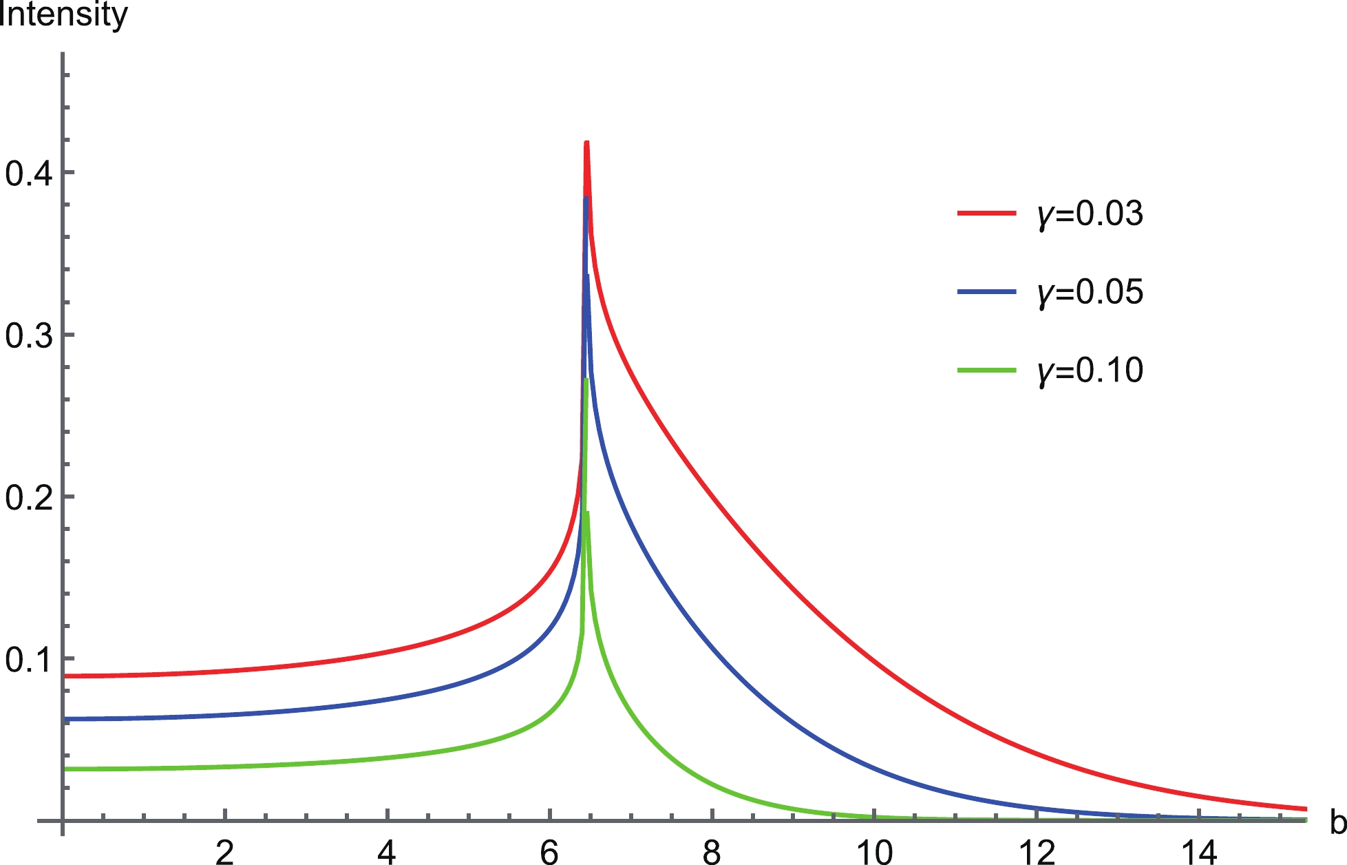
Figure 3. (color online) Specific intensity with static spherical accretion for different γ with
$ \omega_q=-2/3 $ ,$ a=0.1 $ and$ \alpha=0.01 $ .It was deduced that the obtained shadow images are mirror symmetrical when the inclination angle of the observer is complementary to the axisymmetric black holes [76]. For the shadow of the spherically symmetrical black hole, we can choose the position of the observer in the north pole and at the right of the black hole in Fig. 1 and Fig. 2. To keep the images of the shadow in the center of the picture, we can allow the inclination angle of the observer remain
$ 0 $ . The observed specific intensities and shadows for different parameter a are plotted in Fig. 4 with$ \omega_q=-2/3 $ and$ \alpha =0.01 $ . For the specific intensity in Fig. 4 (a), the string clouds parameter a affects the maximum value of specific intensity and the radius of the photon sphere, which is consistent with the analysis in Table 2. As the parameter a increases, the radius of the cosmological horizon$ r_c $ decreases rapidly, which causes the upper limit of the integration to reduce and the lower limit of the integration$ r_h $ to get larger, albeit slowly. The result is that the geodesics of photons shorten rapidly as a increases, which leads to a smaller average specific intensity.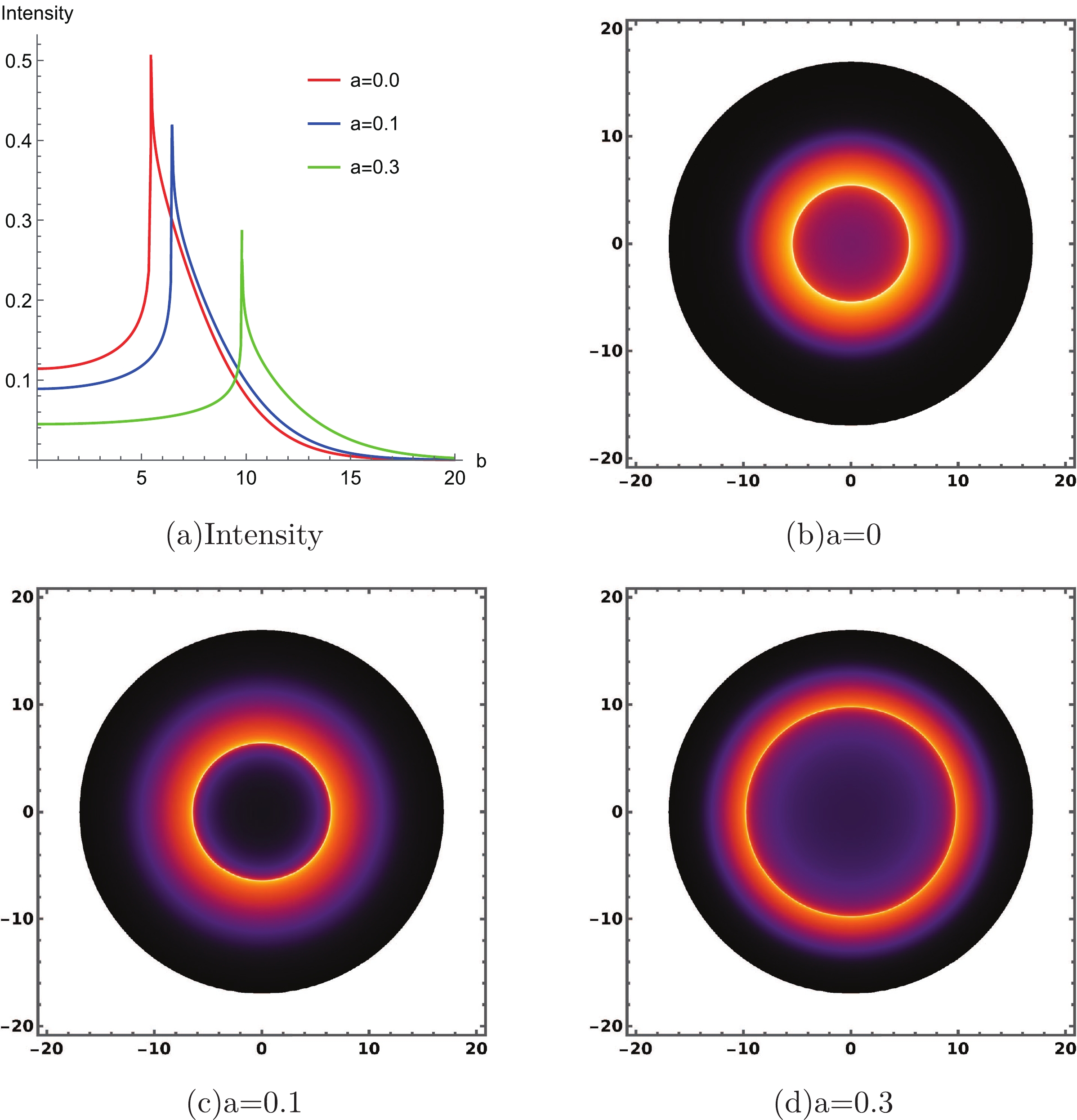
Figure 4. (color online) Specific intensity for different a in Fig. 4 (a) and the black hole shadow with static spherical accretion for different a in other images with
$ \omega_q = -2/3 $ and$ \alpha = 0.01 $ .When
$ b=b_{ph} $ , the photons continue to rotate around the black hole in an unstable circular orbit located at$ r _{ph} $ of the black hole which is called the photon spheres. The impact parameter b stands for the radius of shadow in the eyes of the distant observerer [77]. We can adopt the impact parameter b to represent the radius of shadow and describe the variation in the specific intensity I, which is obtained through an integral along the null geodesic [78]. Fig. 4 presents the black hole shadows for different values of a in the region$ b\leqslant 17 $ . Different colors correspond to different values of the specific intensity, and we demonstrate all the profiles of the shadows with one color function in which a greater specific intensity implies a brighter state, while a smaller one indicates a darker state. We can directly compare the intensity magnitude inside and outside the photon sphere. The shadow is circularly symmetric, and the photon sphere is a bright ring outside the black hole.As the parameter a of string clouds converges to a maximum value, the radius of the shadow approaches the cosmological horizon. When
$ \omega _q=-2/3 $ and$ \alpha =0.01 $ , we obtain$ a<0.612158 $ . From Table 2, we can observe that$ r_c=34.1421 $ and$ b_{ph}=30.0948 $ when$ a=0.6 $ . The observed specific intensity and shadow for$ a=0.6 $ is illustrated in Fig. 5. Most of the specific intensity is concentrated around$ b=b_{ph} $ . Moreover, from the profile of shadow in Fig. 5, it can be observed that all regions are relatively dark except for the vicinity of$ b=b_{ph} $ .
Figure 5. (color online) Specific intensity and the black hole shadow with static spherical accretion for
$ a=0.6 $ ,$ \omega_q = -2/3 $ and$ \alpha = 0.01 $ .Using the same method, we investigated the specific intensities and the shadows for different
$ \omega_q $ values with$ a=0.1 $ and$ \alpha=0.01 $ in Fig. 6. From the image of specific intensity in Fig. 6 (a), it can be observed that$ \omega_q $ would also affect the maximum value of specific intensity and the radius of the photon sphere. As$ \omega_q $ decreases, the radius of the shadow increases. It can be observed from Table 1 that$ r_c=12.5872 $ and$ b_{ph}=7.06308 $ for$ \omega_q=-0.9 $ , which is small; hence, we especially set the region in Fig. 6 (d) to make$ b\leqslant r_c $ . The specific intensity inside the photon sphere does not vanish but has a small finite value, as some photons near the black hole have escaped [58, 72].
Figure 6. (color online) Specific intensity for different
$ \omega_q $ in Fig. 6 (a) and the black hole shadow with static spherical accretion for different$ \omega_q $ in other images with$ a=0.1 $ and$ \alpha = 0.01 $ . -
In this section, the accreting matter is free-falling in a static and spherically symmetric spacetime. When the angular velocity of the black hole is not considered, the accretion matter will only exhibit radial velocity towards the black hole. We still employ Eq. (20) to investigate the shadow. The redshift factor in this model can be expressed as
$ \begin{align} g=\frac{p_{\alpha }u_o^{\alpha }}{p_{\beta }u_e^{\beta}}, \end{align} $

(22) where
$ p_\mu $ is the 4-momentum of photons,$ u^{\mu}_o = (1, 0, 0, 0) $ is the 4-velocity of the distant observer, and$ u^{\mu}_e $ is the 4-velocity of the photons emitted from the accretion. The matter which emits the photons at different locations has different radial velocities owing to the tidal force from the black hole. In the infalling accretion, the$ u^{\mu}_e $ can be expressed as [74]$ \begin{align} u^{t}_e = \frac{1}{A(r)},\quad u^{r}_e = -\sqrt{\frac{1-A(r)}{A(r)B(r)}},\quad u^{\theta}_e = u^{\phi}_e =0. \end{align} $

(23) From Eq. (1), we simply set
$ A(r) = f(r) $ ,$ B(r) = 1/f(r) $ [72]. As$ p_t $ is a constant and$ p_{\alpha}p^{\alpha}=0 $ , we obtain$ \begin{align} p_r = \pm p_t\sqrt{\frac{1}{f(r)}\left(\frac{1}{f(r)} - \frac{b^2}{r^2}\right)}. \end{align} $

(24) Combining Eqs. (22), (23), and (24), the redshift factor can be expressed as
$ \begin{align} g=-\frac{f(r)}{\sqrt{1-f(r)} \sqrt{1-\dfrac{b^2 f(r)}{r^2}}-1}. \end{align} $

(25) We substitute Eqs. (19), (21), and (25) into Eq. (20) to obtain a function of specific intensity that is determined by the impact parameter b; then, we can plot the black hole shadow with an infalling spherical accretion. The shadows for
$ a=0.1 $ and$ a=0.3 $ are drawn in Fig. 7 (b) and Fig. 7 (d), respectively with$ \omega_q=-2/3 $ and$ \alpha=0.01 $ . The interior of the shadows with an infalling spherical accretion will be darker than that with the static spherical accretion. Owing to the radial velocity of the accreting matter, the frequency of the photons we received reduces and the profile of shadow gets darker. The same conclusion can be drawn from Eq. (25).
Figure 7. (color online) Specific intensity with static and infalling spherical accretion for
$ a=0.1 $ and$ a=0.3 $ in Fig. 7 (a) and Fig. 7 (c), respectively. The profile of black hole shadows with an infalling spherical accretion for$ a=0.1 $ and$ a=0.3 $ in Fig. 7 (b) and Fig. 7 (d), respectively, with$ \omega_q=-2/3 $ and$ \alpha=0.01 $ .We are also interested in the difference of the specific intensity between static and infalling spherical accretions. With
$ \omega_q=-2/3 $ and$ \alpha=0.01 $ , we plot the graph of specific intensity with static and infalling spherical accretions for$ a=0.1 $ and$ a=0.3 $ in Fig. 7 (a) and Fig. 7 (c), respectively. As analyzed above, the blue line is significantly lower than the red line in$ b<b_{ph} $ . As b increases, the specific intensity$ I(b) $ with either static or infalling spherical accretion gradually converges, because the emitted photon with larger impact parameter b will move to a smaller average radial position in the integral along the geodesic, and the effect of the redshift factor diminishes. When$ a=0.3 $ in Fig. 7 (c), the difference between the blue and red lines also increases because the observers and black holes get closer, which in turn leads to a larger redshift factor g from Eq. (25).Accordingly, we further investigate how different
$ \omega_q $ impacts the specific intensity with an infalling spherical accretion in Fig. 8. From Table 1, the radius of shadow$ b_{ph} $ varies very slowly with$ \omega_q $ , which causes the bright rings in Fig. 8 (b) and Fig. 8 (d) to have a similar size. For both static and infalling spherical accretions, the specific intensity varies for different$ \omega_q $ values because the length of the optic path varies with$ \omega_q $ .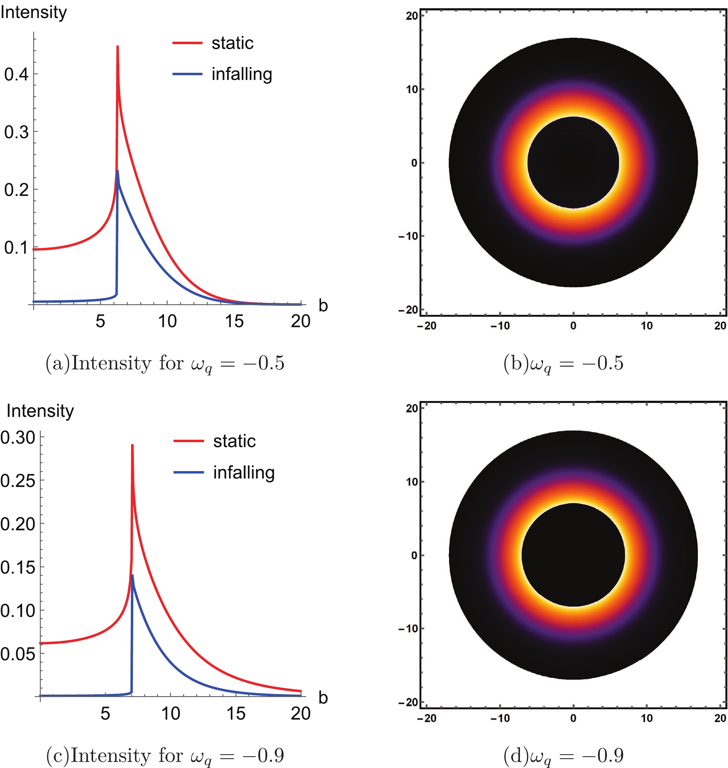
Figure 8. (color online) Specific intensity with static and infalling spherical accretion in Fig. 8 (a) and Fig. 8 (c), respectively. The profile of black hole shadows with an infalling spherical accretion in Fig. 8 (b) and Fig. 8 (d) for
$ \omega_q=-0.5 $ and$ \omega_q=-0.9 $ , respectively, with$ a=0.1 $ and$ \alpha=0.01 $ .Either with static or infalling spherical accretion, the radius of the shadow is the same in both Fig. 7 and Fig. 8; in other words, the peak of the images of specific intensity are all located at
$ b=b_{ph} $ . We can infer that the model of the accretion considered in this study solely affects the value of the specific intensity and not the profile, because the radii of the shadow and photon sphere are actually the intrinsic properties of spacetime. -
We first derived the black hole solution combining quintessence and string clouds, and used the Euler-Lagrangian equation to obtain the geodesics of photons. By analyzing the influence of parameters on photons trajectories, we deduced that the radius of the photon sphere
$ r_{ph} $ is non-monotonic as$ \omega_q $ decreases, which is consistent with previous results [58]. When a increased, the radius of the event horizon$ r_h $ , cosmological horizon$ r_c $ , photon sphere$ r_{ph} $ , and corresponding impact parameter$ b_{ph} $ all varied monotonically. Then, we discussed the range of a in different$ \omega_q $ values. As the photons were deflected, they formed the shadow of a black hole.Moreover, we studied the black hole shadow with static and infalling spherical accretions respectively. The backward ray shooting method helped us obtain the specific intensity
$ I(b) $ from a static observer. For the spherical accretion, we assumed that the density of light sources follows a normal distribution affected by the coefficient γ. In addition, the photons emitted were not strictly monochromatic, whose frequencies conform to the Gaussian distribution with a central frequency$ \nu_* $ and width$ \Delta\nu $ . The photon emissivity was expressed as$ j(\nu_e) $ . Using the backward ray shooting method and the model of the photon emissivity, we plotted the shadow and photon sphere with static and infalling spherical accretions. Owing to the Doppler effect, the interior of the shadow with an infalling spherical accretion will be darker. Different$ \omega_q $ and a values would change the size and intensity of the shadow. Hence, we investigated the emissivity with different coefficients γ and inferred that the intensity will decrease as γ increases.In the presence of the cosmological horizon, the range of a is not arbitrary, which needs to satisfy
$ r_c>b_{ph} $ . Assuming$ r_c<b_{ph} $ , then all photons emitted from the observer will not be able to escape from the black hole, which causes the specific intensity to be small.In fact, there are some flaws in the backward ray shooting method, which implies that when we compare the specific intensity observed at different distances from the black hole, the intensity observed by the distant observer is stronger than that of the closer observer in Fig. 4 (a) and Fig. 6 (a). When the cosmological horizon is not considered, in other words, when the observer's position is fixed, the ray shooting method may appear more realistic. We can also make it more practicable by assuming the observer's position changes with the size of cosmological horizon
$ r_c $ , such as improving the accretion model or applying a more practical frequency distribution function.The EHT Collaboration portrays M87* and claims that the observation supports General Relativity. We expect this to provide novel insights and implications for the quintessence dark energy model, including the string theory from the observations of the black hole shadow in future astronomical observation projects.
-
We are grateful to Peng Wang, Hanwen Feng, Yuchen Huang, Qingyu Gan, and Wei Hong for useful discussions.
Shadow and photon sphere of black hole in clouds of strings and quintessence
- Received Date: 2021-01-06
- Available Online: 2022-06-15
Abstract: In this study, we investigate the shadow and photon sphere of the black bole in clouds of strings and quintessence with static and infalling spherical accretions. We obtain the geodesics of the photons near a black hole with different impact parameters b to investigate how the string cloud model and quintessence influence the specific intensity by altering the geodesic and the average radial position of photons. In addition, the range of the string cloud parameter a is constrained to ensure that a shadow can be observed. Moreover, the light sources in the accretion follow a normal distribution with an attenuation factor γ, and we adopt a model of the photon emissivity


 DownLoad: