


 Abstract
 HTML
HTML Reference
 Related
 PDF
PDF


-
Since physicists predicted that there exists a relatively stable region centered on the proton number
$ Z = 114 $ and neutron number$ N = 184 $ , called the island of stability [1, 2], superheavy nuclei have become one of the most prominent topics in nuclear physics. Several major scientific devices were involved in the synthesis of superheavy nuclei. In the Russian Dubna laboratory, physicists successfully carried out complete fusion reactions with the double magic nucleus$ ^{48} $ Ca beam and various actinide targets and also synthesized novel nuclides with$ Z = 112-118 $ [3-7]. To synthesize the nuclides beyond$ Z = 118 $ , these laboratories, such as GSI in Germany [8-10], Dubna in Russia [11], and RIKEN in Japan [12], have continuously conducted experimental studies on the synthesis of elements$ Z = 119 $ and$ Z = 120 $ using thermal fusion reactions. Unfortunately, the novel nuclides exceeding$ Z = 118 $ are yet to be experimentally synthesized.Owing to the experimental difficulties in synthesizing superheavy nuclei, theoretical studies on superheavy nuclei are necessary, which can provide a guide for experiments. Stability and decay are the two essential attributes of superheavy nuclei. α-decay is the main de-excitation mode of superheavy nuclei. From the α decay chains, physicists can identify superheavy nuclides [13]. The theoretical studies on α-decay can provide knowledge on the stability of superheavy nuclei and α-decay chains [14-16]. To study the α-decay of superheavy nuclei, physicists have developed several theoretical models, which include the generalized liquid drop model (GLDM) [17-19], density-dependent cluster model [20-22], Coulomb and proximity potential model [23-25], and fission-like model [26]. To better describe the α-decay using these models, physicists have proposed different interaction potentials between the α-particle and daughter nucleus, which include the proximity potential [27], Wood-Saxon potential [28], and the potential from the density functional theory [29]. For simplicity, physicists have also proposed several empirical formulas to describe α decay, such as the universal decay law (UDL) formula [30], Royer's formula [31], and Viola-Seaborg formula [32]. These formulas can satisfactorily reproduce the experimental half-lives of α decay.
Spontaneous fission is another important de-excitation method from superheavy nuclei to stable nuclei [33-35]. Because α-decay and spontaneous fission compete with each other in the process of superheavy nuclei de-excitation to stable nuclei, the study of spontaneous fission is also necessary. Compared with α-decay, the spontaneous fission of superheavy nuclei is more complicated and the theoretical description of spontaneous fission is very difficult. Consequently, Swiatecki proposed a semi-empirical formula for the half-lives of spontaneous fission [36]. Recently, based on richer experimental data, physicists have developed several novel empirical formulas for spontaneous fission half-lives [37-40].
In the α-decay and spontaneous fission processes of superheavy nuclei, the shell effect plays an important role [41]. As we know, more stable superheavy nuclei may exist near magic numbers. To consider the shell effect, Strutinsky proposed a method to quantitatively calculate the shell correction from single-particle levels [42]. The method has been widely applied to extract the shell correction based on different models [43, 44]. Recently, the shell correction is introduced in the generalized liquid-drop model, and it improves the description of the α-decay of superheavy nuclei [45, 46].
Although the introduction of the shell corrections can improve the theoretical description for the α-decay of superheavy nuclei, there are systematic deviations between the calculated half-lives and the experimental data, especially near the closed-shell
$ N = 126 $ . The novel relativistic Hartree-Fock (RHF) theory can describe self-consistently stable and exotic nuclei, and it is beneficial to evaluate the shell correction [43].In addition to the shell corrections, the decay energy
$ Q_{\alpha} $ is another important parameter related to α-decay. The α-decay half-lives of superheavy nuclei are sensitive to the$ Q_{\alpha} $ value. Several phenomenological and microscopic models are employed to fit the mass of the nuclei and extract the$ Q_{\alpha} $ value. Comparably, the Weizs$ \ddot{a} $ cker-Skyrme-4 model (WS4) with the radial basis function (RBF) correction [47] is the model with the highest accuracy in describing nuclear mass.Based on these considerations, we apply the RHF theory to calculate the single-particle levels and extract the shell correction. We adopt the
$ Q_{\alpha} $ values from the WS4 model with the RBF correction. Combining the RHF shell correction and the WS4+RBF$ Q_{\alpha} $ values with the GLDM, we calculate the α-decay lifetimes for the known nuclei with$ Z = 106-118 $ . In comparison with the experimental data, an excellent agreement is obtained. Owing to these advantages, we apply the GLDM with the RHF shell correction and WS4+RBF$ Q_{\alpha} $ values to predict the α-decay lifetimes for the unknown superheavy nuclei with$ Z = 118-120 $ . To determine the dominant decay mode from superheavy to stable nuclei, we also calculated the spontaneous fission lifetime for these superheavy nuclei using two empirical formulas. The related results are presented in the following sections.The remainder of this paper is organized as follows. The theoretical framework is introduced in Sec. II. The numerical results and discussions are presented in Sec. III. Then, a summary is given in Sec. IV.
-
To study the α-decay of superheavy nuclei with the GLDM model, we sketch the theoretical formalism. In the GLDM model, the potential barrier is a function of the distance between the center of mass of two fragments; in addition, the penetration probability is calculated using the WKB approximation [18]. The decay constant λ is defined as
$ \lambda = P_{\alpha }v_{0}P, $

(1) where
$ P_{\alpha } $ denotes the preformation factor. Owing to the lack of experimental data for superheavy nuclei, the preformation amplitude is considered the same as that of heavy nuclei. Based on Ref. [48], its value is fixed to$ P_{\alpha } = 0.39 $ for even-even nuclei,$ P_{\alpha } = 0.25 $ for odd-A nuclei, and$ P_{\alpha } = 0.15 $ for odd-odd nuclei via the comparison of theoretical results with experimental data.$ v_{0} $ represents the assault frequency of the α-particle in the parent nucleus, and can be calculated by the formula [49]$ v_{0} = \frac{1}{2R}\sqrt{\frac{2E_{\alpha }}{M}}, $

(2) with the radius of the parent nucleus denoted by R, α-particle energy corrected by recoil
$ E_{\alpha } $ , and mass of the α-particle denoted as M. P is the penetration probability and is calculated with the WKB approximation$ \begin{equation*} P = \exp \left\{ -\frac{2}{\hbar }\int_{r_{\rm{in}}}^{r_{\rm{out}}}\sqrt{ 2\mu \left[ E\left( r\right) -Q_{\alpha }\right] }{\rm d}r\right\} , \end{equation*} $

where
$ E\left(R_{\mathrm{in}}\right) = E\left(R_{\mathrm{out}}\right) = Q_{\alpha } $ . μ,$ Q_{\alpha } $ , and$ E(r) $ denote the reduced mass, decay energy of the α -particle, and penetrating potential barrier of the α-particle, respectively. In the GLDM,$ E(r) $ consists of five parts$ E(r) = E_{\rm V}+E_{\rm S}+E_{\rm C}+E_{\rm{prox}}+E_{\rm{mic}}, $

(3) where
$ E_{\rm V} $ ,$ E_{\rm S} $ ,$ E_{\rm C} $ , and$ E_{\rm{prox}} $ represent the volume, surface, Coulomb, and proximity energies, respectively. More details can be found in Ref. [19].$ E_{\rm{mic}} $ represents the microcosmic corrections of α-decay, which mainly include the shell and pairing energy corrections. In the α-decay process of superheavy nuclei, the pairing energy is shape-dependent, and the detailed calculation can be found in Refs. [50, 51].The shell correction is expressed as [52]:
$ E_{\rm{shell}} = E_{\rm{shell}}^{\rm{sphere}}(1-2.6\alpha ^{2}){\rm e}^{-\alpha ^{2}}, $

(4) where
$ \alpha ^{2} = \bar{(\delta R)^{2}}/a^{2} $ represents the deviation of the deformed nucleus from the spherical nucleus.$ a = 0.32r_{0} $ where$ r_{0} $ denotes the nucleon radius, which is set to 1.2 fm, according to the droplet model of atomic nuclei [52].$ E_{\rm{shell}}^{\rm{sphere} } $ represents the shell correction energy of the spherical nucleus, and is calculated using the Strutinsky shell correction method [42]$ E_{\rm{shell}}^{\rm{sphere}} = \sum\limits_{i = 1}^{N,Z}\varepsilon _{i}-\int_{-\infty }^{\tilde{\lambda}}\varepsilon \tilde{g}(\varepsilon ){\rm d}\varepsilon , $

(5) where
$ \varepsilon _{i} $ represent the energies of single-particle levels,$ \tilde{ \lambda} $ denotes the Fermi energy related to smoothed distribution, and$ \tilde{g }(\varepsilon) $ is the density of levels. In Refs. [44, 46], the single-particle levels are obtained by solving the Schrö dinger equation with an axially deformed Woods-Saxon potential. In this research, the shell correction is extracted from the microscopic single-particle levels in the self-consistent RHF calculations [43]. More details on this can be found in Refs. [53-55]. With the available decay constant λ, the half-live is obtained using$ T_{1/2} = $ ln$ 2/{\lambda } $ .For comparison, we have also calculated the half-lives of the α-decay using the universal decay law (UDL) formula developed in Ref. [30]. The specific expression of UDL formula is
$ \begin{aligned}[b] \log_{10}T_{1/2}({\rm s}) = &aZ_{1}Z_{2}\sqrt{\frac{A_{1}A_{2}}{(A_{1}+A_{2})Q_{ \alpha}}} \\ &+b\sqrt{\frac{A_{1}A_{2}}{(A_{1}+A_{2})}Z_{1}Z_{2}\Big(A_{1}^{ 1/3}+A_{2}^{1/3}\Big)}+c, \end{aligned} $

(6) where the values of the parameters a, b, and c are determined by fitting experimental data.
-
Similar to the α-decay, the spontaneous fission is an essential mode from superheavy nuclei to stable nuclei. Owing to the complexity of spontaneous fission, the calculation of the spontaneous fission's lifetime is considerably difficult. Hence, physicists have proposed several semi-empirical formulas based on nuclear structure. In this study, we choose the two commonly empirical formulas to describe the spontaneous fission half-lives [37, 38], which can optimally reproduce the experimental data.
By considering the strong interaction, Coulomb interaction, and isospin effect, Xu et al. introduced a semi-empirical formula, calculating the half-lives of spontaneous fission for heavy and superheavy nuclei [38], which is expressed as
$ \begin{aligned}[b] T_{1/2}({\rm s}) = \frac{{\rm ln2}}{n\cdot P_{{\rm sf}}} = &\exp \Big[2\pi \Big[c_{0}+c_{1}A+c_{2}Z^{2} +c_{3}Z^{4}\\ &+c_{4}(N-Z)^{2}-\Big(0.13323\frac{Z^{2}}{A^{1/3}}-11.64\Big)\Big]\Big], \end{aligned} $

(7) where
$ c_{0} = -195.09227 $ ,$ c_{1} = 3.10156 $ ,$ c_{2} = -0.04386 $ ,$ c_{3} = 1.40301\times 10^{-6} $ , and$ c_{4} = -0.03199 $ . n denotes the frequency factor chosen as a constant, and$ P_{\rm{sf}} $ represents the penetration probability calculated by the WKB approximation. For convenience, in the following discussions, this formula is called the Xu formula.Considering the isospin and shell correction, Santhosh et al. developed a generalized Swiatecki formula that calculates the half-life of spontaneous fission [37],
$ \begin{aligned}[b] \log_{10}T_{1/2}({\rm yr}) = &a\frac{Z^{2}}{A}+b\left(\frac{Z^{2}}{A}\right)^{2}+c\left( \frac{N-Z}{N+Z}\right) \\ &+d\left(\frac{N-Z}{N+Z}\right)^{2}+eE_{\rm shell}+f, \end{aligned} $

(8) where
$ a = -43.25203 $ ,$ b = 0.49192 $ ,$ c = 3674.3927 $ ,$ d = $ $ -9360.6 $ ,$ e = 0.8930 $ , and$ f = 578.56058 $ .$ E_{\rm{shell}} $ denotes the shell correction energy obtained from the FRDM [56]. For convenience, in the following discussions, this formula is called KPS formula. -
Based on the preceding formalism, we calculate the half-lives of α -decay for the nuclei with
$ Z = 106-118 $ using the GLDM with different shell corrections. The obtained results are presented in Table 1, where the first column labels the parent nuclei happening α-decay, and the second column presents the experimental$ Q_{\alpha} $ values. The fifth, sixth, and seventh columns represent the calculated half-lives of α-decay by the GLDM without shell correction, GLDM with the WS shell correction, and GLDM with the RHF shell correction, respectively. For comparison, the half-lives of α-decay from the UDL formula are presented in the fourth column, and the experimental data are given in the third column.Nucleus $Q_{\alpha}$ (Exp)/MeV

log $_{10}T_{1/2}$ (Exp)/s

log $_{10}T_{1/2}$ (UDL)/s

log $_{10}T_{1/2}$ (GLDM)/s

log $_{10}T_{1/2}$ (GLDM+WS)/s

log $_{10} T_{1/2}$ (GLDM+RHF)/s

$^{269}$ Sg

8.54 2.924 2.063 1.396 2.202 2.963 $^{271}$ Sg

8.67 1.982 1.573 0.931 1.611 2.348 $^{270}$ Bh

9.06 1.785 0.683 0.341 1.040 1.881 $^{271}$ Bh

9.42 0.176 −0.486 −0.942 −0.400 0.431 $^{272}$ Bh

9.21 1.025 0.162 −0.160 0.415 1.155 $^{274}$ Bh

8.94 1.643 1.019 0.594 1.143 1.886 $^{273}$ Hs

9.67 −0.292 −0.888 −1.344 −0.911 −0.096 $^{275}$ Hs

9.45 −0.699 −0.244 −0.783 −0.360 0.448 $^{274}$ Mt

10.20 −0.357 −2.063 −2.167 −1.881 −0.989 $^{275}$ Mt

10.48 −1.699 −2.851 −3.082 −2.807 −1.961 $^{276}$ Mt

10.10 −0.284 −1.811 −1.957 −1.682 −0.802 $^{278}$ Mt

9.58 0.653 −0.298 −0.629 −0.402 0.470 $^{277}$ Ds

10.71 −2.456 −3.128 −3.342 −3.234 −2.274 $^{279}$ Ds

9.85 −0.538 −0.743 −1.273 −1.235 −0.222 $^{281}$ Ds

8.85 1.104 2.467 1.609 1.519 2.522 $^{278}$ Rg

10.85 −2.377 −3.146 −3.124 −3.262 −2.160 $^{279}$ Rg

10.53 −1.046 −2.307 −2.644 −2.792 −1.651 $^{280}$ Rg

9.91 0.623 −0.550 −0.887 −1.018 0.069 $^{281}$ Rg

9.41 1.230 0.989 0.250 0.157 1.148 $^{282}$ Rg

9.16 2.000 1.799 1.205 1.129 1.994 $^{281}$ Cn

10.45 −0.745 −1.745 −2.173 −2.301 −1.367 $^{283}$ Cn

9.66 0.623 0.560 −0.160 −0.223 0.443 $^{285}$ Cn

9.32 1.447 1.625 0.789 0.822 1.229 $^{282}$ Nh

10.78 −1.137 −2.294 −2.428 −2.533 −1.748 $^{283}$ Nh

10.38 −1.125 −1.205 −1.724 −1.799 −1.136 $^{284}$ Nh

10.12 −0.013 −0.467 −0.858 −0.902 −0.392 $^{285}$ Nh

10.01 0.623 −0.155 −0.814 −0.824 −0.516 $^{286}$ Nh

9.79 0.978 0.500 −0.008 0.032 0.251 $^{285}$ Fl

10.56 −1.000 −1.370 −1.879 −1.882 −1.587 $^{286}$ Fl

10.35 −0.921 −0.789 −1.573 −1.545 −1.476 $^{287}$ Fl

10.17 −0.319 −0.280 −0.945 −0.875 −0.950 $^{288}$ Fl

10.07 −0.180 0.003 −0.904 −0.775 −1.019 $^{289}$ Fl

9.98 0.279 0.259 −0.496 −0.292 −0.592 $^{287}$ Mc

10.76 −1.432 −1.585 −2.091 −2.114 −2.152 $^{288}$ Mc

10.65 −0.759 −1.297 −1.624 −1.635 −1.753 $^{289}$ Mc

10.49 −0.481 −0.862 −1.477 −1.438 −1.600 $^{290}$ Mc

10.41 −0.187 −0.648 −1.076 −0.996 −1.186 $^{290}$ Lv

11.00 −2.081 −1.917 −2.596 −2.614 −2.722 $^{291}$ Lv

10.89 −1.721 −1.637 −2.166 −2.154 −2.277 $^{292}$ Lv

10.78 −1.886 −1.351 −2.126 −2.057 −2.205 $^{293}$ Lv

10.71 −1.244 −1.173 −1.795 −1.683 −1.839 $^{293}$ Ts

11.32 −1.658 −2.448 −2.880 −2.876 −2.971 $^{294}$ Ts

11.18 −1.292 −2.098 −2.367 −2.317 −2.419 $^{294}$ Og

11.82 −3.237 −3.370 −3.859 −3.869 −3.941 σ 0.76 1.03 0.92 0.66 Table 1. Half-lives of α-decay for the superheavy nuclei from Sg to Og isotopes. The results obtained from the calculations with the UDL, GLDM, and GLDM with the RHF shell correction and GLDM with the WS shell correction are presented in the forth, fifth, sixth, and seventh columns, respectively. The experimental data [45, 57-60] are displayed in the third column. The RMS of relative deviation between the calculated α-decay half-lives and the experimental data are presented in the last row.
Table 1 shows that the available half-lives of the α-decay in the four different calculations agree well with the experimental data for the nuclei with
$ Z = 106-118 $ . Compared with the UDL formula, the GLDM calculations agree with the experimental data better, especially those with the RHF shell correction. To quantitatively evaluate the accuracy of different models, we calculate the relative deviation between the theoretical α-decay half-lives and experimental data with the formula$ \sigma = \sqrt{\frac{1}{n}\sum\limits_{i = 1}^{n}\left[ \log _{10}\left( T_{1/2}^{\exp ,i}/T_{1/2}^{\rm{cal},i}\right) \right] ^{2}}, $

(9) where σ represents the root mean square (RMS) of relative deviation. The σ value of the GLDM calculation without shell correction is 1.03, while those with the WS and RHF shell corrections are 0.92 and 0.66, respectively. This indicates that the GLDM represents a good description of the α-decay of superheavy nuclei. The experimental half-lives of α-decay are reproduced well in the GLDM calculations with the shell corrections, especially with the RHF shell correction. Namely, the GLDM with the RHF shell correction is more precise in describing the α-decay of superheavy nuclei.
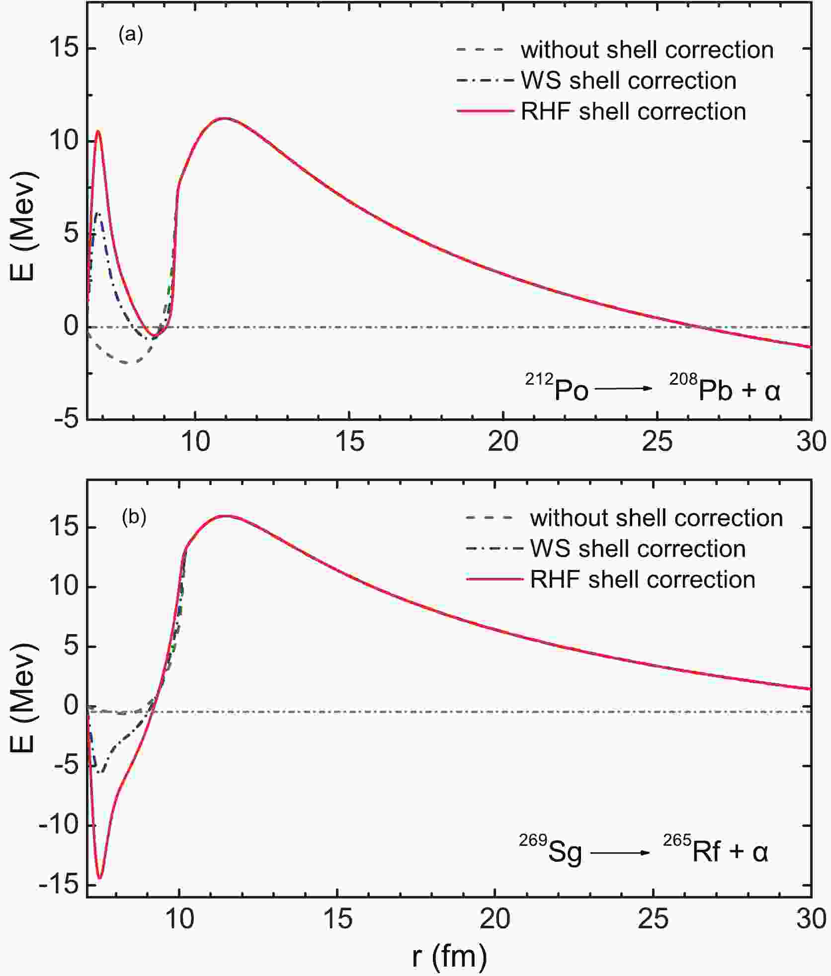
To understand why the shell correction plays an important role in the α-decay of superheavy nuclei, we have plotted the potential barriers of α-decay in the GLDM with different shell corrections. In Fig. 1, the dashed line represents the α-decay barrier in the GLDM without shell correction; the dashed-dotted and solid lines are the α-decay barriers with the WS and RHF shell corrections, respectively. Compared with the results without shell correction, significant changes in the potential barriers in the GLDM with the WS and RHF shell corrections are in the range of
$ r<10 $ fm. In particular, with the RHF shell corrections, the change in the potential barrier is remarkable, which significantly influences the lifetime of α-decay. For the α-decay of$ ^{212} $ Po, the shell correction ensures that the potential of α-decay exhibits a potential barrier in the vicinity$ r = 0 $ . Compared with the WS shell correction, the potential barrier modified by the RHF shell correction is more significant, which improves the prediction of the GLDM model on the half-lives of α-decay in comparison with the experimental data. Similarly, for the α-decay of$ ^{265} $ Rf, there appears a potential well near$ r = 0 $ after considering the shell correction. Compared with the WS shell correction, the potential changed by the RHF shell correction is more remarkable, which results in the calculated half lives of α-decay exhibiting a better agreement with the experimental data. These indicate that the shell correction changes the α-decay potential and improves the theoretical prediction of the α-decay lifetimes. The RHF shell correction changes the α-decay potential more significantly and enables the theoretical prediction to be superior to that of the WS shell correction.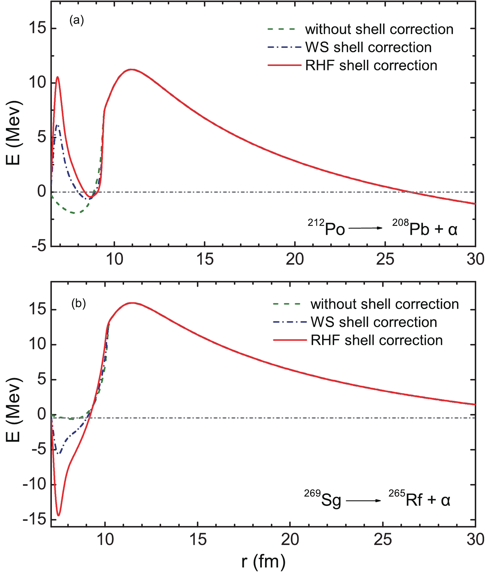
Figure 1. (color online) Potential barriers of α-decay in the GLDM without shell correction, with WS shell correction, and with RHF shell correction. The results for
$ ^{212} $ Po and$ ^{269} $ Sg are displayed in Fig. 1(a) and (b), respectively.To clarify the advantages of the RHF shell correction, we compare the α-decay half-lives with the different shell corrections. The differences between the calculated α-decay half-lives and the experiment data are plotted in Fig. 2, where the results obtained from the GLDM calculations with the WS and RHF shell corrections are presented in Fig. 2 (a) and (b) for the isotopes from Sg to Og. For the GLDM with the RHF shell correction, the differences between the calculated half-lives and experimental data lie in the interval (−0.5, 0.5). For those with the WS shell correction, the differences lie in the interval (−1.5, −0.5). This indicates that the half-lives of α-decay in the GLDM calculations with the RHF shell correction agree with the experimental data better than that with the WS shell correction. Because the RHF is a self-consistent microscopic theory and has gained considerable success in describing stable and exotic nuclei, it is more appropriate to extract the shell correction from the RHF in predicting the half-lives of α-decay using the GLDM.
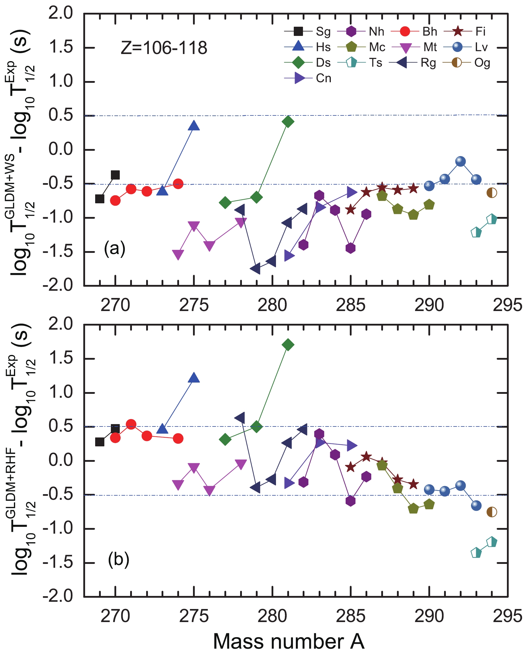
Figure 2. (color online) Differences between the calculated half-lives of α-decay and the experimental data for the nuclei from Sg to Og. The GLDM calculations with the WS and the RHF shell corrections are presented in the upper and lower panels, respectively.
The half-lives of α-decay are sensitive to the decay energy
$ Q_{\alpha} $ . In the recently presented WS4 model [47], by taking into account the surface diffusion correction of unstable nuclei and the radial basis function correction, the RMS deviation between the calculated mass and the experimental data for these 2353 known nuclei decreases to 237 keV. Considering that the WS4+RBF model accurately predicts nuclear mass, we extract the$ Q_{\alpha} $ value from this model. With the$ Q_{\alpha} $ value, we calculate the α-decay half-lives for these 45 isotopes from Sg-Og with the GLDM. To clearly present the calculated results, these 45 isotopes are divided into four groups: even-even, even-odd , odd-even, and odd-odd nuclei. For comparison, the α-decay half-lives are also calculated by the GLDM with the$ Q_{\alpha} $ extracted from the FRDM model. The differences between the calculated half-lives and the experimental data are presented in Fig. 3. Compared with the FRDM model, the deviations between the GLDM calculation with the WS4+RBF model and the experiment data are smaller for even-even, even-odd, odd-even, and odd-odd nuclei. Hence, in the following GLDM calculations,$ Q_{\alpha} $ is extracted from the WS4+RBF model.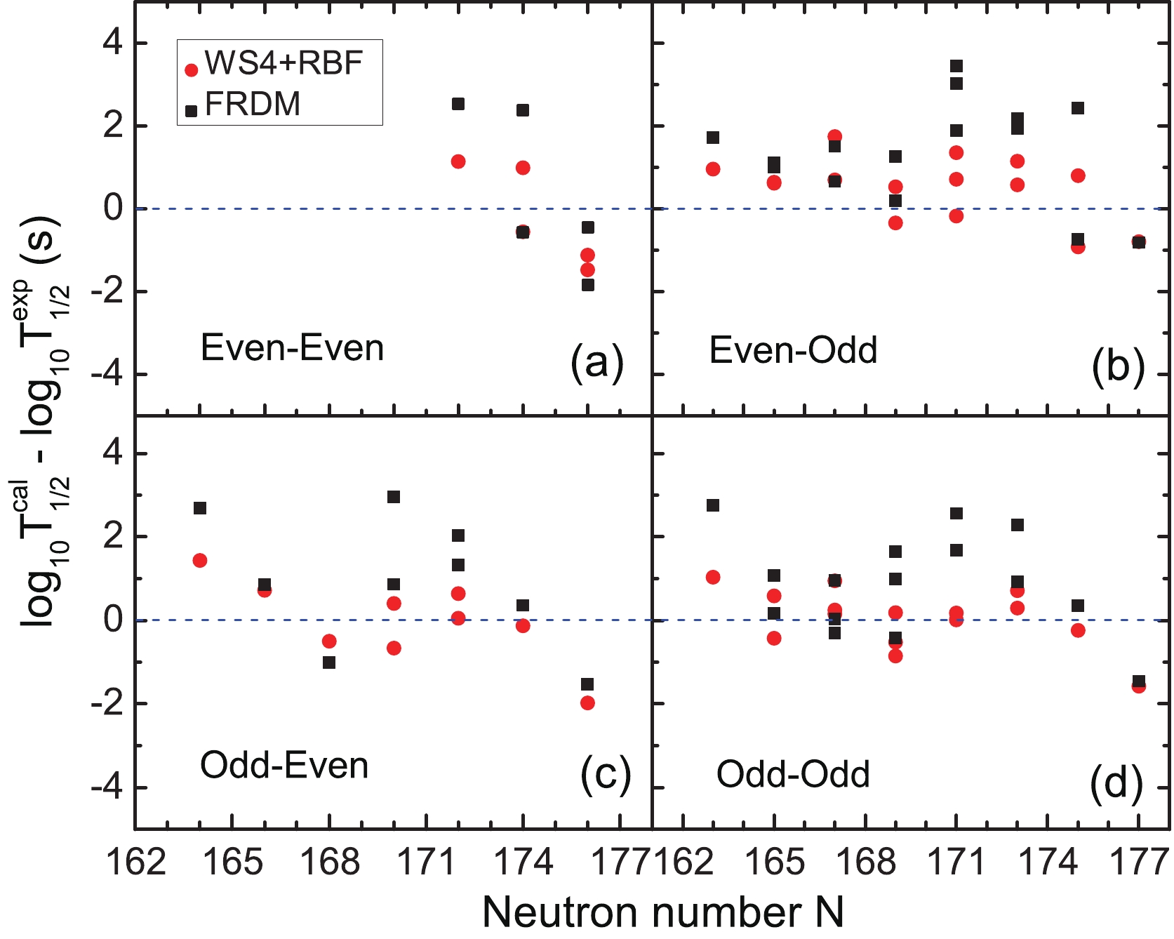
Figure 3. (color online) Differences between the calculated half-lives of α-decay and the experimental data as a function of the neutron number for these nuclei from Sg to Og isotopes. The results for even-even, even-odd, odd-even, and odd-odd nuclei are presented in Fig. 3(a), (b), (c), and (d), respectively.
Previous studies demonstrate that the GLDM with the RHF shell correction is appropriate in describing the α-decay of superheavy nuclei, and the
$ Q_{\alpha } $ value extracted by the WS4+RBF calculations is remarkably consistent with the available data. Hence, it is fascinating to predict the half-lives of α-decay for the unknown superheavy nuclei using the GLDM with the RHF shell correction and the WS4+RBF$ Q_{\alpha } $ values, which is significant in guiding the experimental detection of superheavy nuclei. In the following, we perform the GLDM calculations with the RHF shell correction and the WS4+RBF$ Q_{\alpha } $ value for the superheavy nuclei with$ Z = 118-120 $ . The calculated α-decay half-lives are presented in Fig. 4, where the black circles and red hexagons represent the GLDM without and with the RHF shell correction, respectively. For comparison, the calculated half-lives of α-decay with the UDL formula are displayed as gray pentagons. In addition to the same trend of α-decay half-lives with the neutron number, the available half-lives of α-decay are comparable in the three calculations for the isotopes with$ Z = 118-120 $ . A minimum value emerges at$ N = 186 $ , which implies the important role of magic number in the α-decay. In addition, a sub-minimum vlaue appears at$ N = 180 $ , which may imply a sub-magic number in these superheavy nuclei. Although the available α-decay half-lives are comparable, the impact of the shell correction on the half-lives of α-decay is not negligible in the GLDM calculations. In general, the RHF shell correction depresses the α-decay lifetimes for most of nuclei with$ N<186 $ and increases the α-decay lifetimes for most of the nuclei with$ N>186 $ in the GLDM calculations.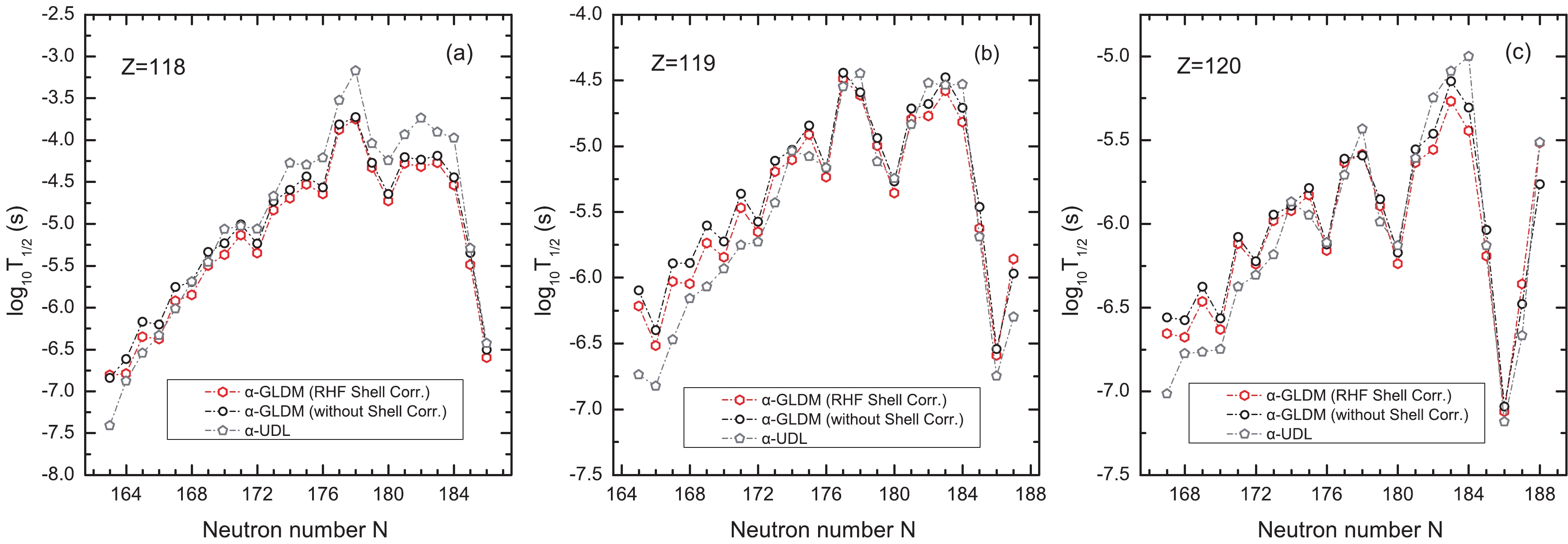
Figure 4. (color online) Calculated α-decay half-lives for the isotopes with
$ Z = 118,119,120 $ . The red hexagons, black circles, and gray pentagons represent the results from the GLDM with the RHF shell correction, the GLDM without shell correction, and the UDL model, respectively. The α-decay half-lives for the isotopes with$ Z = 118 $ ,$ Z = 119 $ , and$ Z = 120 $ are presented in Fig. 4(a), (b), and (c), respectively.Because the results from the GLDM-RHF calculations for the known nuclei are more consistent with the experiment data, as presented in Fig. 2, the GLDM-RHF prediction on the α-decay half-life for these unknown superheavy nuclei should be more reliable. Although the deviations of the α-decay half-life in the calculations with and without shell corrections are quite small, considering that the more reliable the theoretical prediction, the more helpful it is in guiding the experimental detection of superheavy nuclei, the present improvement from the GLDM-RHF calculations is beneficial in exploring superheavy nuclei in experiments.
In addition to the α-decay, the spontaneous fission is one of the most important modes from superheavy to stable nuclei. Considering that the spontaneous fission and α-decay compete with each other, we have also calculated the half-lives of spontaneous fission by using the two commonly adopted empirical formulas: KPS and XU formulas. To save space, we have listed all the calculated half-lives of α-decay and spontaneous fission in the appendix A for the reader's convenience.
To ascertain the dominant process, we have calculated the ratios of the α-decay lifetimes to the spontaneous fission lifetimes for the superheavy nuclei with
$ Z = 118,119,120 $ , as plotted in Fig. 5. It can be observed that the ratios intially decrease up to the minimum value at approximately$ N = 176 $ and then increase with the neutron number. The ratios of the α-decay lifetime to the spontaneous fission lifetimes calculated with KPS formula significantly differ from those with the XU formula. These differences may originate from the shell correction because the shell correction has been considered in the KPS formula but not in the XU formula. This indicates that the shell exerts an important influence on the α-decay and spontaneous fission of superheavy nuclei. In addition, we have also observed the ratios of the α-decay lifetimes to the spontaneous fission lifetimes log$ _{10} (T_{\alpha }/T_{\rm{sf}}) $ to be less than zero, with a few exceptions for the superheavy nuclei with$ Z = 118,119,120 $ , which indicates that the α-decay is the main de-excitation mode from the superheavy to stable nuclei for the superheavy nuclei$ ^{281-304}118 $ ,$ ^{284-306}119 $ , and$ ^{287-308}120 $ .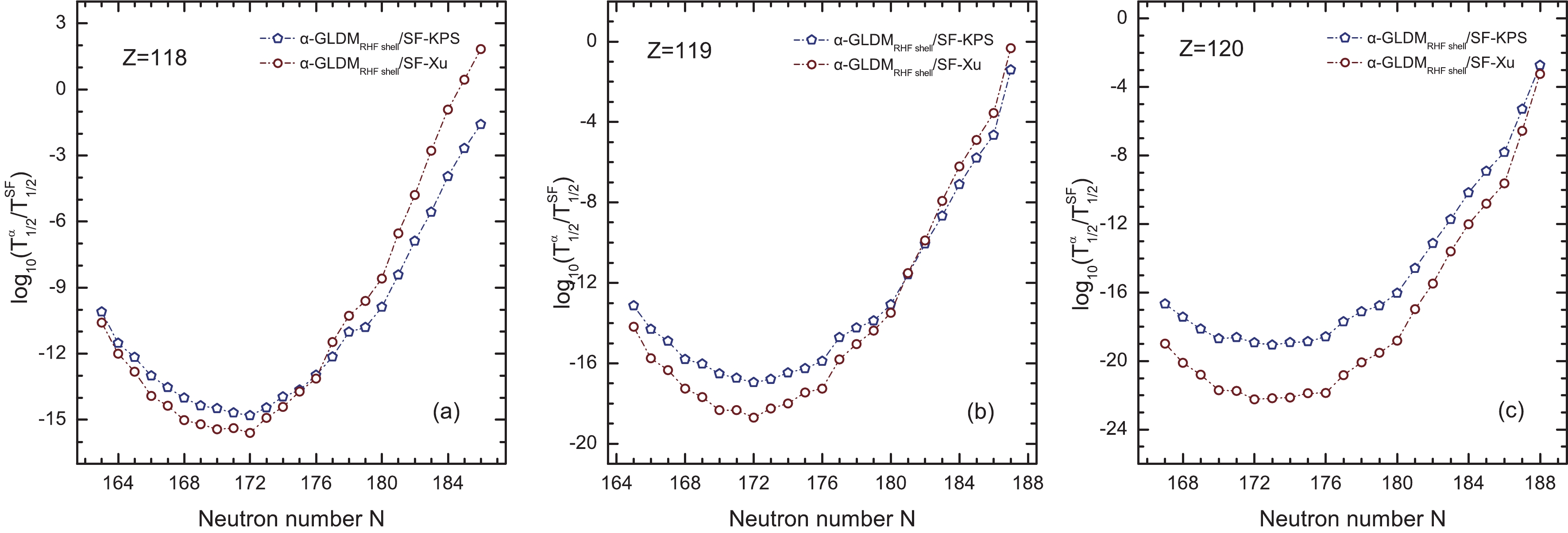
Figure 5. (color online) Ratios of the α-decay lifetime to the spontaneous fission lifetime for the superheavy nuclei with
$ Z = 118,119,120 $ . The α-decay half-lives are calculated by the GLDM with RHF shell correction. The half-lives of spontaneous fission are calculated by the KPS and Xu formulas. The results for the superheavy nuclei with$ Z = 118 $ ,$ Z = 119 $ , and$ Z = 120 $ are presented in Fig. 5(a), (b), and (c), respectively. -
The generalized liquid-drop model with the microscopic shell correction from the relativistic Hartree-Fock calculations was adopted to explore the α-decay of superheavy nuclei. The known nuclei with
$ Z = 106-118 $ were chosen as examples for testing. The calculated half-lives of α-decay agreed well with the experimental data. Compared with the UDL formula, GLDM calculations without shell correction, and GLDM calculations with WS shell correction, the GLDM with the RHF shell correction exhibited the best description for the α-decay of superheavy nuclei.The shell corrections play an important role because the α -decay is clarified. Compared with the calculations without shell correction, the α-decay potential was significantly modified by shell corrections, especially for the RHF shell correction. For the α-decay of
$ ^{212} $ Po ($ ^{265} $ Rf), the shell correction ensured that the α -decay potential exhbited a barrier (well) in the vicinity$ r = 0 $ . Compared with the WS shell correction, the potential barrier (well) modified by the RHF shell correction was sharper, which resulted in the theoretical prediction of the GLDM+RHF being superior to that of the WS shell correction.In the GLDM calculations with the RHF shell correction, the available half-lives agreed with the experimental data better than those with the WS shell correction. The differences between the calculated half-lives of α -decay with the RHF shell correction and the experimental data for the isotopes from Sg to Og were evident in the interval (−0.5, 0.5), while those with the WS shell correction were evident in the interval (−1.5, −0.5). This indicates that the RHF shell correction is superior to the WS shell correction in describing the α-decay of superheavy nuclei.
The influence of the
$ Q_{\alpha} $ value on the α-decay was analyzed. It was determined that the$ Q_{\alpha} $ values from the WS4 model with the radial basis function correction matched the experimental data better than the values from other models.Combining these advantages of the RHF shell correction and the WS4+RBF, the GLDM+RHF with the WS4+RBF
$ Q_{\alpha } $ values was adopted to predict the α -decay lifetime for the unknown superheavy nuclei with$ Z = 118-120 $ . The available half lives of α-decay according to the neutron number exhibited the same trend in comparison with those from the GLDM without shell correction and the UDL formula. A minimum value appeared at$ N = 186 $ , which implied the important role of magic number in the α-decay, including a sub-minimum value at$ N = 180 $ , which could be a sub-magic number in the superheavy nuclei. Compared with the GLDM calculations without shell correction, the RHF shell correction depressed the α-decay lifetime for most nuclei with$ N<186 $ and increased the α-decay lifetime for most nuclei with$ N>186 $ . Compared with the half-lives of spontaneous fission, which are calculated with the two commonly used empirical formulas, it was determined that the α-decay is dominant in the superheavy nuclei$ ^{281-304}118 $ ,$ ^{284-306}119 $ , and$ ^{287-308}120 $ . These results are beneficial in guiding the experimental detection of superheavy nuclei. -
In this section, all the calculated α-decay half-lives are presented in Table A1, where the α-decay half-lives from the GLDM with the RHF shell correction are listed in the third column. For comparison, the α-decay half-lives calculated with the UDL formula are presented in the fourth column. The half-lives of spontaneous fission calculated with the KPS and Xu formulas are presented in the fifth and sixth columns of Table A1, respectively.
$ A$ 

$ Q_{\alpha}/\mathrm{MeV}$ 

$ \log _{10} T_{1 / 2}^{\alpha}/{\rm s}$ 

$ \log _{10} T_{1 / 2}^{\mathrm{sf}}/{\rm s}$ 

WS4+RBF GLDM+RHF UDL KPS Xu Z=118 281 13.77 −6.805 −7.411 3.294 3.782 282 13.49 −6.788 −6.877 4.739 5.216 283 13.32 −6.348 −6.543 5.819 6.472 284 13.21 −6.376 −6.333 6.636 7.548 285 13.05 −5.921 −6.015 7.612 8.446 286 12.89 −5.850 −5.691 8.161 9.165 287 12.77 −5.497 −5.457 8.866 9.705 288 12.59 −5.368 −5.064 9.122 10.067 289 12.56 −5.135 −5.026 9.557 10.250 290 12.57 −5.349 −5.062 9.468 10.254 Continued on the next page Table A1. Calculated half-lives of α-decay and spontaneous fission for the superheavy nuclei with Z = 118–120. The half-lives of α-decay are calculated by the GLDM with the RHF shell correction and the UDL formula. The half-lives of spontaneous fission are calculated by the two commonly used empirical formulas. The
$ Q_{\alpha}$ of α-decay are obtained from the WS4 model with the RBF corrections.Table A1-continued from the previous page $ A$ 

$Q_{\alpha}/\mathrm{MeV}$ 

$ \log _{10} T_{1 / 2}^{\alpha} /{\rm s}$ 

$ \log _{10} T_{1 / 2}^{\mathrm{sf}}/{\rm s} $ 

WS4+RBF GLDM+RHF UDL KPS Xu 291 12.39 −4.835 −4.671 9.625 10.079 292 12.21 −4.694 −4.274 9.273 9.726 293 12.21 −4.528 −4.295 9.118 9.194 294 12.17 −4.643 −4.210 8.333 8.484 295 11.88 −3.875 −3.523 8.269 7.596 296 11.73 −3.749 −3.171 7.266 6.528 297 12.08 −4.327 −4.039 6.480 5.283 298 12.16 −4.728 −4.243 5.161 3.859 299 12.02 −4.280 −3.935 4.143 2.256 300 11.93 −4.316 −3.737 2.570 0.476 301 12.00 −4.271 −3.904 1.302 −1.483 302 12.02 −4.538 −3.975 −0.587 −3.621 303 12.58 −5.489 −5.293 −2.812 −5.936 304 13.10 −6.598 −6.428 −5.011 −8.430 305 12.89 −5.856 −5.987 −7.621 −11.102 306 12.46 −5.176 −5.061 −10.006 −13.952 307 11.90 −3.770 −3.778 −12.244 −16.981 308 11.18 −2.285 −1.967 −14.478 −20.187 309 10.70 −0.842 −0.652 −16.552 −23.572 310 10.41 −0.250 0.162 −19.019 −27.135 311 10.08 0.892 1.150 −21.208 −30.875 312 9.74 1.699 2.221 −23.804 −34.794 313 8.63 5.603 6.180 −26.146 −38.891 314 8.37 6.379 7.236 −28.820 −43.165 315 8.28 6.870 7.570 −28.066 −47.618 316 8.60 5.390 6.257 −30.687 −52.249 317 8.53 5.953 6.536 −33.048 −57.057 318 8.40 6.333 7.054 −38.137 −62.043 319 8.28 7.032 7.523 −40.641 −67.207 320 9.15 3.693 4.142 −43.424 −72.549 321 9.00 4.390 4.659 −46.226 −78.069 322 8.89 4.588 5.075 −49.404 −83.767 323 8.71 5.373 5.720 −53.598 −89.642 324 8.47 6.036 6.666 −56.699 −95.695 325 8.24 7.061 7.611 −59.663 −101.926 326 8.12 7.264 8.095 −62.890 −108.334 327 7.91 8.234 8.979 −65.145 −114.920 328 7.60 9.349 10.425 −68.661 −121.684 329 7.31 10.790 11.803 −71.633 −128.625 330 7.15 11.301 12.618 −74.978 −135.744 Continued on the next page Table A1-continued from the previous page $ A$ 

$Q_{\alpha}/\mathrm{MeV}$ 

$ \log _{10} T_{1 / 2}^{\alpha}/{\rm s}$ 

$ \log _{10} T_{1 / 2}^{\mathrm{sf}}/{\rm s}$ 

WS4+RBF GLDM+RHF UDL KPS Xu 331 6.94 12.547 13.732 −77.125 −143.041 332 6.76 13.572 14.717 −80.670 −150.515 333 6.77 13.891 14.652 −84.032 −158.166 334 6.57 14.966 15.764 −87.702 −165.996 335 6.26 17.119 17.655 −91.213 −174.002 336 6.07 18.202 18.875 −94.690 −182.186 337 5.72 20.879 21.295 −97.846 −190.548 338 5.35 23.553 24.109 −101.251 −199.087 339 5.25 24.643 24.927 −104.503 −207.803 Z=119 284 13.56 −6.215 −6.738 6.928 7.969 285 13.60 −6.516 −6.825 7.797 9.231 286 13.42 −6.028 −6.472 8.870 10.315 287 13.26 −6.047 −6.159 9.764 11.219 288 13.20 −5.737 −6.069 10.305 11.945 289 13.13 −5.844 −5.932 10.682 12.492 290 13.04 −5.469 −5.753 11.273 12.860 291 13.02 −5.653 −5.729 11.304 13.050 292 12.87 −5.194 −5.431 11.608 13.061 293 12.69 −5.105 −5.036 11.375 12.893 294 12.70 −4.913 −5.079 11.356 12.547 295 12.73 −5.236 −5.166 10.662 12.022 296 12.45 −4.488 −4.549 10.232 11.319 297 12.40 −4.613 −4.448 9.632 10.437 298 12.69 −4.997 −5.118 8.889 9.376 299 12.74 −5.357 −5.247 7.721 8.138 300 12.55 −4.794 −4.834 6.800 6.720 301 12.40 −4.771 −4.520 5.287 5.125 302 12.40 −4.579 −4.536 4.097 3.351 303 12.39 −4.818 −4.531 2.292 1.399 304 12.91 −5.625 −5.690 0.171 −0.732 305 13.40 −6.591 −6.749 −1.935 −3.041 306 13.18 −5.857 −6.298 −4.452 −5.528 307 12.76 −5.241 −5.412 −6.352 −8.193 308 12.04 −3.526 −3.772 −8.115 −11.037 309 11.35 −2.161 −2.053 −10.249 −14.058 310 10.86 −0.710 −0.748 −12.215 −17.258 311 10.76 −0.624 −0.475 −14.593 −20.636 312 10.56 0.131 0.075 −16.702 −24.192 313 9.37 3.407 3.865 −19.192 −27.926 Continued on the next page Table A1-continued from the previous page $ A$ 

$Q_{\alpha}/\mathrm{MeV}$ 

$ \log _{10} T_{1 / 2}^{\alpha}/{\rm s}$ 

$ \log _{10} T_{1 / 2}^{\mathrm{sf}}/{\rm s}$ 

WS4+RBF GLDM+RHF UDL KPS Xu 314 8.97 4.940 5.281 −21.446 −31.838 315 8.65 5.861 6.504 −24.069 −35.928 316 8.67 5.978 6.419 −26.488 −40.196 317 9.20 3.807 4.394 −29.167 −44.642 318 9.13 4.375 4.661 −31.728 −49.266 319 8.98 4.746 5.202 −34.545 −54.068 320 8.83 5.545 5.747 −36.947 −59.047 321 8.68 5.901 6.317 −39.861 −64.205 322 8.50 6.780 6.988 −42.509 −69.540 323 7.93 8.866 9.406 −45.533 −75.053 324 8.60 6.362 6.577 −48.306 −80.744 325 8.77 5.409 5.877 −51.416 −86.613 326 8.79 5.523 5.820 −54.246 −92.659 327 8.47 6.390 7.045 −57.482 −98.884 328 8.23 7.458 8.024 −60.588 −105.285 329 7.87 8.650 9.604 −63.231 −111.865 330 7.67 9.668 10.540 −66.232 −118.622 331 7.65 9.382 10.582 −68.196 −125.557 332 7.57 10.062 10.964 −71.338 −132.669 333 7.44 10.720 11.594 −74.825 −139.959 334 7.29 11.864 12.339 −78.085 −147.427 335 7.07 12.908 13.451 −81.653 −155.072 336 7.10 13.047 13.310 −85.010 −162.894 337 6.34 17.211 17.656 −88.645 −170.894 338 6.23 18.210 18.368 −91.853 −179.072 339 5.89 20.325 20.645 −95.186 −187.427 Z=120 287 13.84 −6.655 −7.016 10.012 12.336 288 13.71 −6.678 −6.775 10.766 13.426 289 13.69 −6.464 −6.765 11.675 14.337 290 13.68 −6.630 −6.750 12.063 15.070 291 13.48 −6.119 −6.376 12.504 15.624 292 13.44 −6.241 −6.306 12.687 15.999 293 13.37 −5.981 −6.184 13.080 16.195 294 13.22 −5.922 −5.869 12.997 16.213 295 13.25 −5.828 −5.948 13.040 16.052 296 13.32 −6.160 −6.112 12.425 15.713 297 13.12 −5.632 −5.709 12.073 15.195 298 12.98 −5.585 −5.434 11.532 14.498 299 13.23 −5.893 −5.989 10.884 13.623 Continued on the next page Table A1-continued from the previous page $ A$ 

$Q_{\alpha}/\mathrm{MeV}$ 

$ \log _{10} T_{1 / 2}^{\alpha}/{\rm s}$ 

$ \log _{10} T_{1 / 2}^{\mathrm{sf}}/{\rm s}$ 

WS4+RBF GLDM+RHF UDL KPS Xu 300 13.29 −6.238 −6.130 9.801 12.569 301 13.04 −5.635 −5.608 8.947 11.337 302 12.87 −5.557 −5.247 7.572 9.927 303 12.79 −5.268 −5.088 6.465 8.338 304 12.74 −5.444 −5.000 4.734 6.571 305 13.26 −6.192 −6.129 2.722 4.625 306 13.77 −7.121 −7.182 0.689 2.501 307 13.50 −6.360 −6.667 −1.060 0.199 308 12.95 −5.516 −5.513 −2.782 −2.281 309 12.14 −3.678 −3.692 −4.438 −4.940 310 11.48 −2.367 −2.059 −6.484 −7.776 311 11.18 −1.400 −1.270 −8.371 −10.791 312 11.20 −1.612 −1.342 −10.653 −13.984 313 11.01 −0.931 −0.835 −12.649 −17.356 314 10.74 −0.480 −0.099 −15.062 −20.905 315 9.41 3.573 4.088 −17.195 −24.632 316 9.17 4.151 4.933 −19.689 −28.538 317 9.91 1.949 2.373 −22.025 −32.621 318 9.91 1.703 2.365 −24.646 −36.882 319 9.83 2.239 2.627 −27.107 −41.322 320 9.66 2.623 3.168 −29.815 −45.939 321 9.51 3.326 3.661 −32.207 −50.734 322 9.35 3.676 4.208 −35.049 −55.707 323 9.10 4.728 5.096 −37.697 −60.858 324 7.98 8.857 9.653 −40.775 −66.186 325 7.70 10.202 10.916 −43.335 −71.693 326 9.27 3.792 4.424 −46.474 −77.377 327 8.67 6.069 6.701 −49.146 −83.239 328 8.50 6.407 7.346 −52.340 −89.279 329 8.60 6.091 6.919 −55.181 −95.497 330 8.39 6.572 7.763 −58.337 −101.892 331 8.09 7.861 9.044 −59.574 −108.465 332 7.99 7.991 9.478 −62.830 −115.216 333 7.95 8.627 9.648 −65.879 −122.144 334 7.91 8.810 9.806 −69.275 −129.250 335 7.74 9.932 10.564 −72.470 −136.533 336 6.53 16.236 16.994 −75.974 −143.994 337 6.29 17.967 18.475 −79.232 −151.633 338 6.35 17.494 18.124 −82.786 −159.449 339 7.55 11.161 11.441 −86.137 −167.442
Research on α-decay for the superheavy nuclei with Z = 118–120
- Received Date: 2020-12-08
- Available Online: 2022-05-15
Abstract: The generalized liquid-drop model (GLDM) with the microscopic shell correction from relativistic Hartree-Fock (RHF) calculations is used to explore the α-decay of superheavy nuclei. The known nuclei with


 DownLoad: