


 Abstract
 HTML
HTML Reference
 Related
 PDF
PDF


-
Charmonium physics lives in an energy regime where both the perturbative and nonperturbative features of quantum chromodynamics (QCD) intertwine. Notably, charmonium decay played an important role in establishing the asymptotic freedom of QCD and functioned as a clean platform for probing the interplay between perturbative and nonperturbative dynamics. In particular, the two photon annihilation rates of charmonium are significantly beneficial in elucidating quark-antiquark interactions and decay mechanisms [1, 2].
In this research, we study the two-photon decay width of
$ \chi_{c0} $ , which has been extensively studied from both experimental and theoretical approaches. From the experimental approach, using the decay of$ \psi(3686)\rightarrow $ $ \gamma\chi_{c0},\chi_{c0}\rightarrow \gamma\gamma $ , both CLEO-c and BESIII collaborations reported results of the two-photon decay width$ \Gamma_{\gamma\gamma}(\chi_{c0}) $ [3, 4]:$ \begin{aligned}[b] \Gamma^{\rm CLEO-c}_{\gamma\gamma}(\chi_{c0}) = & 2.36(35)_{\rm{stat}}(22)_{\rm{syst}}\, {\rm{keV}} \\ \;\ \Gamma^{\rm BESIII}_{\gamma\gamma}(\chi_{c0}) = & 2.03(8)_{\rm{stat}}(14)_{\rm{syst}}\, {\rm{keV}} \\ \quad\; \Gamma^{\rm PDG}_{\gamma\gamma}(\chi_{c0}) =& 2.20(22) {\rm{keV}} \end{aligned} $

(1) where the first line is obtained from CLEO-c, the second from BESIII, and the last line is the PDG quoted value with combined errors. It is expected that more accurate results for these decay widths will become available in the near future.
On the theoretical side, it is fair to infer that the situation is far from satisfactory. Theoretical results for the decay rate have been obtained using a non-relativistic approximation [5, 6], potential model [7], relativistic quark model [8-11], non-relativistic QCD (NRQCD) factorization [12-18], effective Lagrangian [19], and Dyson-Schwinger equations (DSEs) [20], as well as quenched [21] and unquenched lattice calculations [22]. These results are presented in Table 1, which are scattered quite significantly, although all they fall in the right ballpark. Note that within the framework of NRQCD, the leading-order (LO) prediction is close to the experimental measurements; however, this process is extremely sensitive to high-order QCD radiative corrections and relativistic corrections. Therefore, only the LO predictions are listed in Table 1.
Theoretical computations for $ \Gamma_{\gamma\gamma}(\chi_{c0}) $ /keV

Huang [1] 3.72 $ \pm $ 1.10

Barbieri [12] 3.5 Barnes [6] 1.56 Schuler [17] 2.50 Gupta [7] 6.38 Lanseberg [19] 5.00 Ebert [8] 2.90 Chen [20] 2.06-2.39 Godfrey [9] 1.29 Crater [23] 3.34-3.96 Bodwin [10] 6.70±2.80 Wang [24] 3.78 Münz [11] 1.39±0.16 Laverty [25] 1.99-2.10 Dudek [21] 2.41(58)stat(86)syst CLQCD [22] 0.93(19)stat Table 1. Some theoretical predictions for
$ \Gamma_{\gamma\gamma}(\chi_{c0}) $ .In the last line of Table 1, we list two existing lattice QCD results so far. The first one from Dudek et al. is a quenched lattice computation on a single lattice spacing [21]. The systematic error they quote mainly come from quenching. The second one from CLQCD is an unquenched study using
$ N_f = 2 $ twisted mass fermions at two distinct lattice spacings. The authors found that the lattice artifacts are substantial and only quoted results from a finite lattice spacing, without an error estimate of the finite lattice spacing errors. The number quoted in Table 1 is the result from the finer lattice spacing [22]. Therefore, in both lattice studies, systematic effects such as finite lattice errors are not fully investigated, which was found to be large in the second study [22]. Evidently, in order to fully compare with the upcoming experiments, one needs to work in a theoretical framework that allows an improvable error control, and in this respect, lattice computation has an advantage over other phenomenological methods listed in Table 1.In this study, we attempt to improve on the existing lattice computation of
$ \Gamma_{\gamma\gamma}(\chi_{c0}) $ in two major aspects. First, in previous lattice studies, many systematic effects were not yet completely considered, the most important of them being the finite lattice spacing effect, which was observed in Ref. [22]. Second, it is typical to compute the off-shell form factors at various discrete photon virtualities. To obtain the physical decay width, an extrapolation of these results are required, thereby introducing a model-dependent systematic error.In this study, we have made the following improvements. First, to attack the lattice artifacts, we perform our calculation on ensembles with three different lattice spacings, which enables us to perform a reliable continuum extrapolation. Second, we adopt a novel method to directly extract the on-shell form factor, by-passing the conventional momentum extrapolation and therefore avoiding the corresponding model-dependent extrapolation errors. We also considered the excited-state contamination, further improving our results on the physical form factor. Similar procedures have been successfully utilized for the two-photon decay of
$ \eta_c $ [26]. We expect that these improvements would also shed some light on the two-photon decay of$ \chi_{c0} $ .The remainder of this paper is organized as follows. In Sec. II, the methodology for extracting the on-shell form factor is introduced. Sec. III is divided into several parts. In Sec. III.A, information on the configurations and operators used in this work is introduced. In Sec. III.B, the mass spectrum of
$ \chi_{c0} $ is presented. In Sec. III.C, we provide the renormalization factor and spectrum weight factor. In Sec. III.D, numerical results of the form factor in three different lattice spacings are presented. Then, in Sec. III.F, extrapolation of the results to continuum is performed, yielding our final results for the decay rate. We also compare our results with both the experimental and theoretical results. The main sources of error in our work are discussed, and possible solutions in the future are proposed. -
In this section, we outline the methodology for the calculation of the two-photon decay width of
$ \chi_{c0} $ . In the conventional approach [27], using the Lehmann-Symanzik-Zimmermann (LSZ) reduction formula and integrating out the QED part to${\cal{O}}(\alpha_{em}) $ , the amplitude for the two-photon decay of charmonium can be obtained as follows [21],$ \begin{aligned}[b] \langle\gamma\gamma|M(p_f)\rangle\sim & e^2\epsilon^*_\mu\epsilon^*_\nu\int {\rm d}t_i {\rm e}^{- \omega_1 (t_i -t)}\int {\rm d}^3 \vec{x}\, {\rm e}^{-{\rm i}\vec{p_f}.\vec{x}} \\& \times \int {\rm d}^3 \vec{y}\, {\rm e}^{{\rm i}\vec{q_2}.\vec{y}}\langle 0 | T\Big\{ \varphi_{M}(\vec{x}, t_f) J_\nu(\vec{y}, t) J_\mu(\vec{0}, t_i)\Big\}|0\rangle ,\end{aligned} $

(2) where
$ \varphi_{M}(\vec{x},t_f) $ is an appropriate composite operator that creates a desired meson M (in our case, the$ \chi_{c0} $ meson) from the QCD vacuum;$ \epsilon_{\mu},\epsilon_{\nu} $ denote the polarization four-vectors for the two final photons;$ J_\mu = \sum_qe_q\,\bar{q}\gamma_\mu q $ ($ e_q = 2/3,-1/3,-1/3,2/3 $ for$ q = u,d,s,c $ ) represents the electromagnetic current operator due to the quarks, with e being the elementary charge unit. In this work, we only consider the connected contributions emerging from the charm quark current. Disconnected contributions are neglected. These contributions are extremely expensive for lattice computations and are assumed to be small in charmonium physics [21, 28, 29]. Subsequently, the matrix element in Eq. (2) relevant for the$ \chi_{c0} $ decay can be parameterized in terms of the form factor$ G(Q_1^2,Q_2^2) $ as,$ \begin{aligned}[b] & \langle\gamma(q_1) \gamma(q_2) |M(p_f)\rangle \\ =& \dfrac{2}{m_{\chi}}\left(\dfrac{2}{3} e\right)^2 G\big(Q_1^2,Q_2^2\big)\left[\epsilon_1\cdot\epsilon_2q_1\cdot{q_2}-\epsilon_2\cdot{q_1}\epsilon_1\cdot{q_2}\right], \end{aligned} $

(3) where
$ q_1,\;q_2 $ are the two four-momenta of the final photons while$ Q^2_1 = -q^2_1,\;Q^2_2 = -q^2_2 $ represent the virtualities of the two photons. The mass of$ \chi_{c0} $ is denoted as$ m_\chi $ , and the polarization vectors of the two photons are given by$ \epsilon_1 $ and$ \epsilon_2 $ . The physical decay width is related to the on-shell form factor, which is obtained by a momentum extrapolation towards the physical point:$ Q^2_1 = Q^2_2 = 0 $ . Hence, in this conventional approach, to achieve better control on the extrapolation, one needs to compute the matrix element at various different non-physical virtuality combinations, which also introduces extra computational costs. The extrapolation itself also triggers model-dependent systematic errors. In the novel approach introduced in this study, we adopt a method that requires no off-shell form factor calculations at all and therefore by-passes the model-dependent extrapolation in photon virtualities. This method has been successfully utilized in two-photon decays of$ \eta_c $ [26]. Next, we briefly outline the major steps for the case of$ \chi_{c0} $ below.First, the on-shell decay amplitude of
$ \chi_c\rightarrow 2\gamma $ is related to an infinite-volume hadronic tensor${\cal{F}}_{\mu\nu}(p) $ , which is the Fourier transform of the real-space tensor${\cal{H}}_{\mu\nu}(t,\vec{x}) $ in continuum Euclidean space,$ \begin{aligned}[b] {\cal{F}}_{\mu\nu}(p) =& \int {\rm d}t {\rm e}^{m_\chi t/2}\int {\rm d}^3 \vec{x} {\rm e}^{-{\rm i}\vec{p}\cdot\vec{x}}{\cal{H}}_{\mu\nu}(t,\vec{x})\;,\\{\cal{H}}_{\mu\nu}(t,\vec{x}) =& \left\langle {0\left| {T{J_\mu }(x){J_\nu }(0)} \right|{\chi _{c0}}(k)} \right\rangle \;, \end{aligned} $

(4) where we have chosen the rest-frame of the
$ \chi_{c0} $ meson, such that$ k = (im_\chi, \vec{0}) $ . Note that we have fixed the four-momentum for one of the final photons to be$ p = (im_\chi/2,\vec{p}) $ with$ |\vec{p}| = m_\chi/2 $ , making it explicitly on-shell, and then the energy-momentum conservation guarantees that the other photon with the four-momentum$ p^\prime $ is also on-shell. With this choice, the on-shell decay amplitude can be expressed as$ M = e^2\epsilon^*_\mu(p,\lambda)\epsilon^*_\nu(p^\prime,\lambda^\prime){\cal{F}}_{\mu\nu}(p). $

(5) According to the quantum number of
$ \chi_{c0} $ , the hadronic tensor can be parameterized as (repeated indices are summed),$ {\cal{F}}_{\mu\nu}(p) = \epsilon_{ij\mu\alpha}\epsilon_{ij\nu\beta}p_\alpha k_\beta F_{\chi_{c0}\gamma\gamma}. $

(6) Here, the approach to extracting the on-shell form factor
$ F_{\chi_{c0}\gamma\gamma} $ is also slightly different from the conventional approach. By further multiplying the Lorentz structure factor in the above equation, the hadronic tensor can be contracted to a scalar, including only the form factor$ F_{\chi_{c0}\gamma\gamma} $ with a constant factor. Then, the form factor can be derived by dividing the coefficient as follows,$ \begin{aligned}[b] F_{\chi_{c0}\gamma\gamma} =& \frac{\epsilon_{ij\mu\alpha}\epsilon_{ij\nu\beta}p_\alpha k_\beta{\cal{F}}_{\mu\nu}(p)}{\epsilon_{ij\mu\alpha}\epsilon_{ij\nu\beta}p_\alpha k_\beta\epsilon_{i'j'\mu\alpha'}\epsilon_{i'j'\nu\beta'}p_{\alpha'} k_{\beta'}}\\ =& -\frac{1}{8m_{\chi}|\vec{p}|^2}\int {\rm d}t{\rm e}^{m_\chi t/2}\\ & \times\int {\rm d}^3\vec{x}{\rm e}^{-{\rm i}\vec{p}\cdot\vec{x}}\epsilon_{ij\mu\alpha}\epsilon_{ij\nu0}\frac{\partial{\cal{H}}_{\mu\nu}(x)}{\partial x_{\alpha}}.\end{aligned} $

(7) To date, all derivations are in the continuum Euclidean space. Now, we utilize the spatial isotropy symmetry to average over the spatial direction of
$ \vec{p} $ ,$ \begin{aligned}[b]& {{\rm e}^{ - {\rm i}\vec p \cdot \vec x}} \to \frac{1}{{4\pi }}\int {\rm d} {\Omega _{\vec p}}{{\rm e}^{ - {\rm i}\vec p \cdot \vec x}} = \frac{{\sin (|\vec p||\vec x|)}}{{|\vec p||\vec x|}} \equiv {j_0}(|\vec p||\vec x|)\\& \quad \frac{\rm d}{{{\rm d}z}}({j_0}(z)) = - \left( {\frac{{\sin z}}{{{z^2}}} - \frac{{\cos z}}{z}} \right) \equiv - {j_1}(z), \end{aligned} $

(8) where
$ j_n(x) $ represent the spherical Bessel functions. Finally, the scalar from factor is expressed as$ \begin{aligned}[b] {F_{{\chi _{c0}}\gamma \gamma }} =& \frac{1}{{8{m_\chi }}}\int {\rm d} t{{\rm e}^{{m_\chi }t/2}}\int {{{\rm d}^3}} \vec x\\ & \times \left[ {\frac{{{j_1}(|\vec p||\vec x|)}}{{|\vec p||\vec x|}}({x_i}{{\cal H}_{0i}} + {x_i}{{\cal H}_{i0}}) + \frac{{{j_0}(|\vec p||\vec x|)}}{{|\vec p|}}2{{\cal H}_{ii}}} \right], \end{aligned} $

(9) where
$ i = 1,2,3 $ take spatial indices and are assumed to be summed over.To obtain the hadronic tensor
${\cal{H}}_{\mu\nu}(t,\vec{x}) $ in Eq. (9), we utilize the variational method to determine the optimal interpolation operators and create the$ \chi_{c0} $ meson state [30]. The physical decay width of$ \chi_{c0} $ is given by$ \Gamma_{\gamma\gamma}(\chi_{c0}) = \alpha^2\pi m_{\chi_{c0}}^3F_{\chi_{c0}\gamma\gamma}^2\;. $

(10) Therefore, one only needs to compute the Euclidean correlation functions
${\cal{H}}_{0i} $ and${\cal{H}}_{ii} $ that are directly relevant for the on-shell amplitude and then substitute the results into Eq. (9) to arrive at the physical decay width$ \Gamma_{\gamma\gamma}(\chi_{c0}) $ in Eq. (10). This completely avoids the on-shell extrapolation process in the conventional lattice approach. -
We utilize three
$ N_f = 2 $ -flavor twisted mass gauge field ensembles generated by the Extended Twisted Mass Collaboration (ETMC) with lattice spacing$ a \simeq 0.0667, $ $ 0.085,\;0.098 $ fm, respectively. The parameters of these ensembles are presented in Table 2. The valence charm quark mass parameter$ \mu_c $ is tuned, such that the mass of the$ \eta_c $ meson for each ensemble reproduces its correct physical value. For more details, we refer the reader to Refs. [31, 32],Ensemble a/fm $ L^3\times T $ 

$ N_{ \rm{conf}} $ 

$ a\mu_l $ 

$ m_\pi $ /MeV

$ t_h $ 

Ens. I 0.067(2) $ 32^3\times 64 $ 

$ 179 $ 

0.003 300 10-20 Ens. II 0.085(3) $ 24^3\times 48 $ 

$ 200 $ 

0.004 315 10-15 Ens. III 0.098(3) $ 24^3\times 48 $ 

$ 216 $ 

0.006 365 10-15 Table 2. From left to right, we present the ensemble names, lattice spacing a, spatial and temporal lattice sizes L and T, number of measurements of the correlation function for each ensemble
$ N_{ \rm{conf}}\times T $ , light quark mass$ a\mu_l $ , pion mass$ m_\pi $ , and the range of the time separation$ t_h $ between$ \chi_{c0} $ and the photon.Before getting into the simulation details, we need to clarify an outstanding subtlety related to the twisted mass fermion. Because the twisted mass action breaks parity
${\cal{P}} $ by${\cal{O}}(a^2) $ effects, the basis operator${\cal{O}}_1 = \bar{c}c $ for$ \chi_{c0} $ would unfortunately mix with${\cal{O}}_2 = \bar{c}\gamma^5c $ , which has the opposite parity. This mixing implies that a specific combination of these operators will be relevant in creating a physcial scalar charmonium in the twisted mass action [30]$ {\cal{O}}^\dagger_{\chi_{c0}} = v^{\chi}_{1}{\cal{O}}^\dagger_1 + v^{\chi}_{2}{\cal{O}}^\dagger_{2}. $

(11) The two-point correlation function
$ C_{\chi_{c0}}(t) = \left\langle 0 \right|{\cal{O}}_{\chi_{c0}}(t) $ $ {\cal{O}}^\dagger_{\chi_{c0}}(0)\left| 0 \right\rangle $ can be derived by multiplying the corresponding coefficients with the basis correlation functions$ C'_{ij} = \left\langle 0 \right|{\cal{O}}_i(t){\cal{O}}^\dagger_{j}(0)\left| 0 \right\rangle (i,j = 1,2) $ . Therefore, after choosing a time slice$ t_0 $ , one could disentangle the mixing of the two operators by solving a generalized eigenvalue problem (so-called GEVP procedure):$ \begin{aligned}[b] & \left( {\begin{array}{*{20}{c}} {{{C'}_{11}}(t)}&{{{C'}_{12}}(t)}\\ {{{C'}_{21}}(t)}&{{{C'}_{22}}(t)} \end{array}} \right)\left( {\begin{array}{*{20}{c}} {v_1^\chi }&{v_1^\eta }\\ {v_2^\chi }&{v_2^\eta } \end{array}} \right)\\ =& \left( {\begin{array}{*{20}{c}} {{\lambda _1}}&0\\ 0&{{\lambda _2}} \end{array}} \right)\left( {\begin{array}{*{20}{c}} {{{C'}_{11}}({t_0})}&{{{C'}_{12}}({t_0})}\\ {{{C'}_{21}}({t_0})}&{{{C'}_{22}}({t_0})} \end{array}} \right)\left( {\begin{array}{*{20}{c}} {v_1^\chi }&{v_1^\eta }\\ {v_2^\chi }&{v_2^\eta } \end{array}} \right), \end{aligned}$

(12) where the generalized eigenvalues
$ \lambda_i $ behave like$ {\rm e}^{-E_i(t-t_0)} $ at large time separations. In practice, we fix$ t_0 = 1 $ and solve Eq. (12) on each time-slice independently and then employ them to reconstruct the three-point correlation functions. -
Because the generalized eigenvalues in Eq. (12) decay exponentially, the corresponding mass eigenvalues can be extracted easily from
$ \cosh(m_n) = \frac{\lambda_n(t-1)+\lambda_n(t+1)}{2\lambda_n(t)}. $

(13) Because we want to extrapolate the form factor and eliminate the excited state contamination, we adopt the following two-state fit form for the
$ \chi_{c0} $ correlator,$ C^{(2)}_{\chi_{c0}}(t) = V \sum\limits_{i = 0,1}\frac{Z_i^2}{2m_i} \left({\rm e}^{-m_it}+{\rm e}^{-m_i(T-t)}\right) $

(14) with V being the spatial volume,
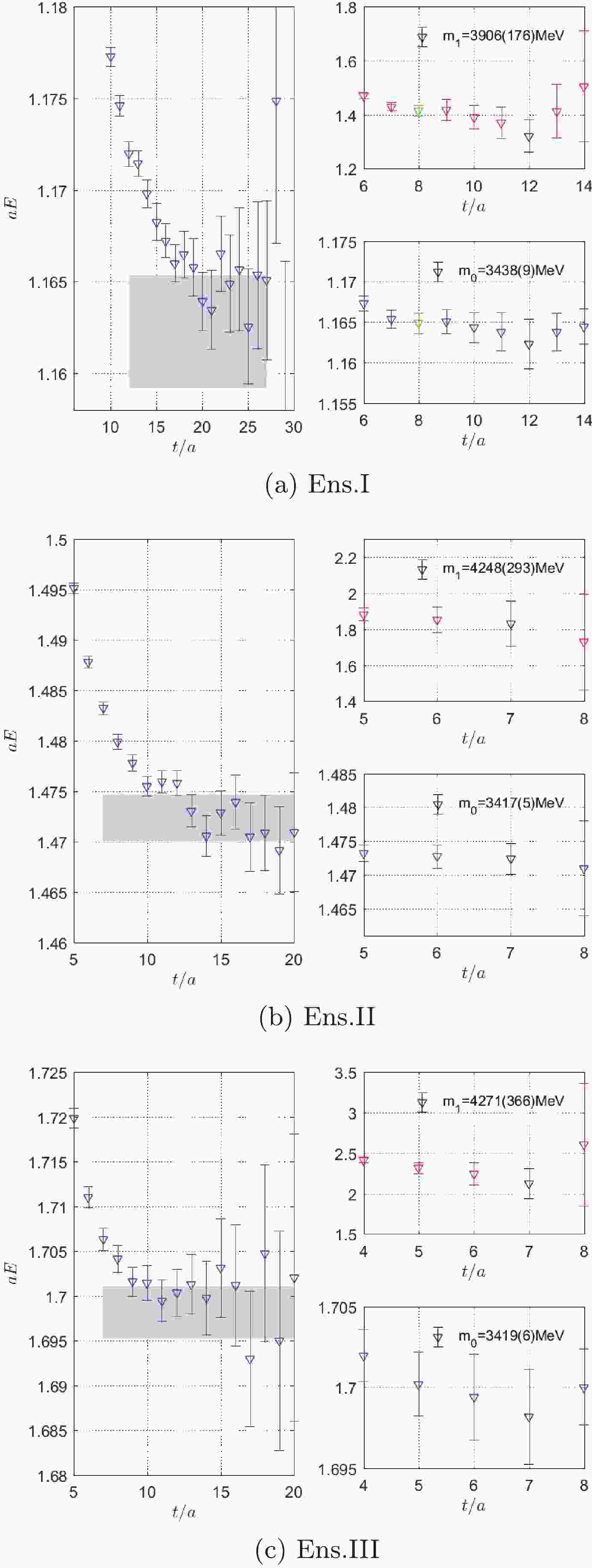
$ m_0 $ the ground state mass, and$ m_1 $ the first excited state mass. The factors$ Z_i = \dfrac{1}{\sqrt{V}}\langle i|{\cal{O}}_{\chi_{c0}}^\dagger|0\rangle $ (with$ i = 0,1 $ ) are the overlap amplitudes for the ground and the first excited state, respectively. The corresponding mass plateaus and masses are illustrated in Fig. 1 for the three ensembles utilized in this work. The left column of the panels show the effective mass on each time slice. The right panels present the mass values fitted from two-point correlation functions, the upper panel for the first excited state, and the bottom one for the ground state. According to the grey bands in the left panels, the starting time slices are adjusted according to$ \chi^2/d.o.f $ of the fit, while the ending time slices are fixed to be$ t_{\max} = 27, 20, 20 $ for ensembles I, II, and III, respectively. Note that the grey band of Ens. I significantly differs from those of the other two ensembles; hence, the ground state mass$ m_0 $ might be underestimated. Therefore, we calculate the result for another plateau with a green mark and take their difference as the major source of systematic uncertainty.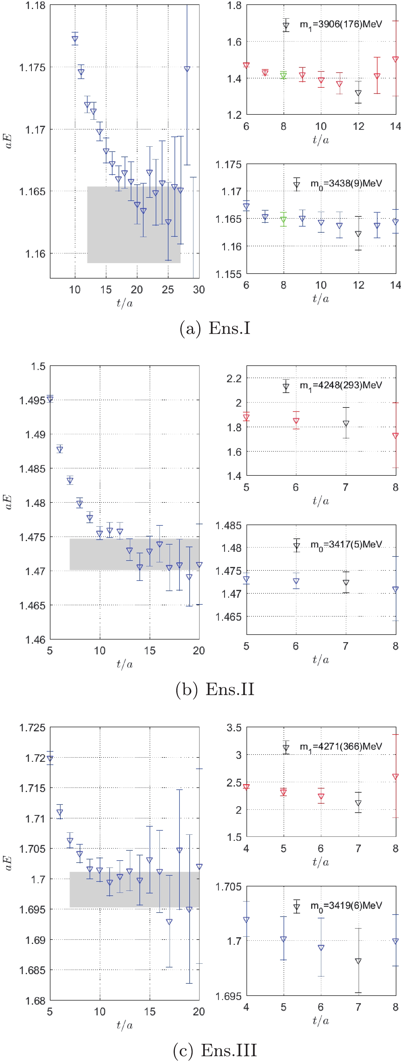
Figure 1. (color online) The left panels present the effective mass at different time slices together with the corresponding fitting ranges (grey bands), while the right panels show the ground and excited state mass values fitted from two-point correlation functions using Eq. (14). The black symbols denote the chosen
$ m_0 $ that corresponds to the grey band to its left. The green symbols in (a) denote another choice for$ m_0 $ and$ m_1 $ .The results for the mass values are summarized in Table 3. Note that we use the
$ \eta_c $ mass to fix the valence charm quark mass$ a\mu_c $ in this study. Furthermore, the$ \chi_{c0} $ experiment mass is 3414.7(3) MeV, as quoted by PDG [33].$ m_0 $ /MeV

$ Z_0 $ 

$ m_1 $ /MeV

Ens. I(a) 3438(9) 0.0959(25) 3906(176) Ens. I(b) 3445(4) 0.0972(9) 4181(57) Ens. II 3417(5) 0.1216(10) 4248(293) Ens. III 3419(6) 0.1320(7) 4271(366) Table 3. Mass value
$ m_0 $ and spectral weight$ Z_0 $ for the ground state and the first excited state mass$ m_1 $ on each ensemble, respectively. Ens. I(a) and Ens. I(b) correspond to the black and green symbols, respectively. -
The hadronic tensor
${\cal{H}}_{\mu\nu} $ contains the electromagnetic current operators$ J_\mu $ from all flavor of quarks. However, becuase we neglect the disconnected diagrams in this study, we only need to consider the charm quark current$ J^{(c)}_\mu = \bar{c}\gamma_\mu c(\vec{x},t) $ . Because we adopt the local current form, there exists an extra multiplicative renormalization factor$ Z_V $ that can be calculated by a ratio of the two-point function and the three-point function expressed in Eq. (15). In principle, this renormalization factor does not depend on the particle state used to calculate it. For a better signal, we decide to adopt the$ \eta_c $ correlators instead of$ \chi_{c0} $ . Considering the around-of-world effect, we use the following relationship to extract$ Z_V $ .$ Z_V = \frac{\sum_{\vec{x}}\langle{\cal{O}}_{\eta_c}(t){\cal{O}}^\dagger_{\eta_c}(0)\rangle}{\sum_{\vec{x}}\langle{\cal{O}}_{\eta_c}(t)J_0^{(c)}(t/2,\vec{x}){\cal{O}}^\dagger_{\eta_c}(0)\rangle}\frac{1}{(1+{\rm e}^{-m_0(T-2t)})}. $

(15) The results for
$ Z_V $ are presented in Table 4.Ens. I Ens. II Ens. III $ Z_V $ 

0.6523(21) 0.6296(29) 0.6057(27) Table 4. Renormalization factor
$ Z_V $ for three ensembles.When computing the scalar form factor
$ F_{\chi_{c0}\gamma\gamma} $ in Eq. (9) on the lattice, the integration over space-time are replaced by discrete summations. When two identical currents in${\cal{H}}_{\mu\nu}(t,\vec{x}) $ , which implies that they share the same Lorentz index, are at the same space-time point, an extra renormalization is required to take the contact term into account . This is owing to a novel type of composite operator that is not properly renormalized yet, even if each current is already properly renormalized by the factor$ Z_V $ . To take this effect into account, one needs to impose another appropriate renormalization condition for this novel composite operator. In this study, we decide not to sum the same space-time point contributions for identical currents, thereby avoiding this potential renormalization. To summarize, the above mentioned procedures adopted on already$ O(a) $ -improved ensembles will at most introduce an extra$ O(a^2) $ lattice artifact on physical observables, which will be considered in the final continuum extrapolation. -
When computing the hadronic tensor, we evaluate the three-point correlation function
$ \langle J_\mu(x)J_\nu(0){\cal{O}}^\dagger_{\chi_{c0}}(-t_h)\rangle $ . To generate the static meson state, we employ the$ Z_4 $ -stochastic wall source placed at time-slice$ -t_h $ . This cuts the uncertainty by approximately half when compared with the simple point source for the meson mass. We also apply the APE [34] and Gaussian smearing [35] for the gauge field and$ \chi_{c0} $ operator. We utilize the random point source propagator for the current to arrive at the three-point correlation function. In practice, the hadronic tensor with current$ J_\nu(0) $ placed at the zero point is actually an average of all the time slices and random positions on each time slice.Consequently, the scalar form factor we computed according to Eq. (9) on the lattice
$ F'_{\chi_{c0}\gamma\gamma} $ actually suffers from excited state contamination owing to the higher excitation states of$ \chi_{c0} $ . What we really need is the ground state$ \chi_{c0} $ . This effect can be addressed by considering the$ t_h $ dependence of the form factors. Therefore, we compute several different separations$ t_h $ and perform the following fit,$ F'_{\chi_{c0}\gamma\gamma}(t_h) = \ F_{\chi_{c0}\gamma\gamma}+\xi\cdot {\rm e}^{-(m_1-m_0)t_h}\;, $

(16) where
$ F_{\chi_{c0}\gamma\gamma} $ and ξ represent the two free parameters. For the parameters$ m_0 $ and$ m_1 $ , we take the values presented in Table 3. The form factors with different time separations$ t_h $ together with the ground state extrapolation values for$ F_{\chi_{c0}\gamma\gamma} $ for three set of ensembles are presented in Fig. 2.
Figure 2. (color online) The left column represents the plateaus of the form factors with different
$ t_h $ while the right column presents the extrapolation to the ground state contribution. The labels (a) and (b), (c) and (d), and (e) and (f) are for Ens. I(a), Ens. II, and Ens. III, respectively. -
The most recent lattice computation on
$ \chi_{c0}\rightarrow \gamma\gamma $ decay in the literature is the one from CLQCD [22], which coincidentally employed the exact same set of ensembles as this research. This allows a more detailed comparison on the level of dimensionless form factors for each of the common lattice spacings. Accordingly, we decide to convert our results for$ F_{\chi_{c0}\gamma\gamma} $ into dimensionless quantities that can be taken as either$ \Gamma_{\gamma\gamma}(\chi_{c0})/m_{\chi_{c0}} $ or the dimensionless form factor$ G(0,0) $ utilized in Ref. [22]. The relationship between these two dimensionless quantities is easily found to be$ \frac{\Gamma_{\gamma\gamma}(\chi_{c0})}{m_{\chi_{c0}}} = \alpha^2 \pi |m_{\chi_{c0}}F_{\chi_{c0}\gamma\gamma}|^2 = \alpha^2 \pi (e_c)^4|G(0,0)|^2. $

(17) Dimensionless quantities have the advantage of being independent of the scale setting process for the lattice spacings, which is subject to its own errors depending on how the scale was set. Because the scale setting processes for lattice calculations have also progressed over the years, information on the lattice spacing in physical units, both the central values and the errors, also keeps changing with time, even for a given particular ensemble. Therefore, it is better to attach these errors due to scale-setting at the very end when comparing with the experiments. In the intermediate step, when comparing with other lattice computations, it is easier to directly compare the dimensionless quantities if possible. In fact, this allows us to compare with previous lattice results in Ref. [22] at each individual lattice spacing, namely Ens. I and Ens. II, which have also been utilized. Certainly, when quoting the final physical decay width, the effect of scale setting will be considered together with its associated errors.
In Table 5, the dimensionless form factor
$ G(0,0) $ obtained via Eq. (17) from$ F_{\chi_{c0}\gamma\gamma} $ for all three ensembles are presented together with the corresponding results for Ens. I and Ens. II from Ref. [22]. Ens. III was not utilized in the study prsented in Ref. [22]. Two entries for Ens. I, labelled as Ens. I(a) and Ens. I(b), correspond to the two different ways of extracting$ \chi_{c0} $ masses, as demonstrated in Fig. 1. The errors quoted for$ G(0,0) $ in this study are obtained using the conventional jackknife method. Regarding the three errors for the results from Ref. [22], they represent errors from statistics, momentum extrapolations, and estimates of the finite lattice spacing errors, respectively. We observe that the central values for dimensionless form factors$ G(0,0) $ differ by almost a factor of two for Ens. I and Ens. II. The reason for this apparent discrepancy remains unknown to us. One possibility could be the under estimation of the lattice artifacts for each of the ensemble in Ref. [22].$ G(0,0) $ 

Ens. I(a) Ens. I(b) Ens. II Ens. III This work 0.1884(123) 0.1899(69) 0.1911(85) 0.1931(131) Ref. [22] 0.09079(8)(19)(90) 0.1017(7)(102)(126) − Table 5. Dimensionless form factors
$ G(0,0) $ obtained in this study and those obtained in Ref. [22] for each ensemble. Ens.I(a) and Ens.I(b) denote two different results obtained by taking two different$ \chi_{c0} $ mass values, as demonstrated in Fig. 1. Ensemble III was not available in Ref. [22]. Errors quoted for$ G(0,0) $ in this study are purely statistical and are obtained using the conventional jackknife method. The three errors for the results from Ref. [22] are the errors from statistics, momentum extrapolations. and estimates for the finite lattice spacings, respectively. -
After obtaining the dimensionless form factors for three different lattice spacings, we can investigate the continuum limit of this quantity. To achieve this, we perform this extrapolation using the more physical quantity
$ \Gamma_{\gamma\gamma}(\chi_{c0})/m_{\chi_{c0}} $ , which is proportional to the norm-squared dimensionless form factor$ |G(0,0)|^2 $ , as indicated in Eq. (17). The continuum extrapolation is done by performing a linear fit in$ a^2 $ for the three ensembles; in addition, the results after the continuum extrapolation, together with the results for each ensemble, are illustrated in Fig. 3. Here the horizontal error bars for the data points indicate the errors in$ a^2 $ inferred from Refs. [31, 32]
Figure 3. (color online) Continuum extrapolation for the ratio
$ \Gamma_{\gamma\gamma}(\chi_{c0})/m_{\chi_{c0}} $ . The three data points with both horizontal and vertical error-bars are the results from the three ensembles. The extrapolated results are represented by two side-by-side points near$ a^2 = 0 $ . The one with a smaller error bar (the right one) represents the extrapolation result without considering lattice spacing errors. The other one (left one) is the result with lattice spacing errors taken into consideration. The data point (blue) below these two with a smaller error depicts the PDG-fit value for this ratio. At the upper right corner, we have also indicated the result of the width in physical units.It is observed that the three data points fit well on a straight line yielding a reasonable
$ \chi^2/d.o.f $ . The two points near$ a^2 = 0 $ with larger error bars designate two different results obtained from the fit with and without considering the horizontal$ a^2 $ -errors for the lattice spacings. Below the two data points, we also plot the corresponding experimental value from PDG for this ratio. The two extrapolated results share almost identical central values. They differ only by their errors. The point with a slightly larger error (the one slightly to the left) is the one that takes the horizontal$ a^2 $ -errors into account, while the other one is the one without considering$ a^2 $ -errors. Finally, there is another source of systematic errors that emerges from the different plateaus in the mass, as discussed in Sec. III. B. Therefore, we finally express the result of the decay width in physical units as$ \Gamma_{\gamma\gamma}(\chi_{c0}) = 3.65(83)_{\rm{stat}}(21)_{\rm{lat.syst}}(66)_{\rm{syst}}\, {\rm{keV}}, $

(18) where the first two errors represent the error obtained without/with the
$ a^2 $ -errors. It should be interpreted as follows: the first error is the error without considering$ a^2 $ -errors. The second one with the subscript$ \rm{lat.syst} $ indicates the extra amount of error if the$ a^2 $ -errors are considered. In other words, one could add the first two errors in quadrature to obtain the error with$ a^2 $ -errors taken into consideration, which is demonstrated by the left point near$ a^2 = 0 $ in Fig. 3. The last error with subscript$ \rm{syst} $ reflects the systematic error from different mass plateaus in Ens. I(a) and Ens. I(b). Accordingly, we separate different sources of systematic errors that have been studied in this research.It is evident that the central value for the decay width obtained in this study is larger than the PDG value. However, owing to our large statistical and systematical uncertainties, it remains compatible with the experimental results within 1.3σ.
We have attempted to estimate the systematic uncertainties that might influence our final result expressed above in Eq. (18). This includes choosing different plateaus for the mass, renormalization factor
$ Z_V $ , spectral weight factor$ Z_i $ , and number of time-slices we adopted for the extrapolation of the ground state form factor. Ultimately, only the two plateaus presented in Sec. III. B contribute to a visible deviation in the central value, which we add in the third error in Eq. (18).Certainly, there are also other sources of systematic errors that are more difficult to quantify, e.g., neglecting the disconnected contributions, quenching the strange and charm quarks, etc. The contributions of the disconnected diagrams are believed to be suppressed in the charmonium system [28, 29] owing to the Okubo-Zweig-Iizuka (OZI) rule. Furthermore, the non-physical masses of up and down quarks usually solely result in a negligible effect, which is indicated in previous lattice calculations [36]. Therefore, the major direction in future improvements points to the deduction of the statistical noise in
$ \chi_{c0} $ correlation functions. Only after the large statistical uncertainty is fully under control, should we consider other remaining systematic effects.Part of the large statistical error in our study can be traced back to the mixing of
$ \chi_{c0} $ and$ \eta_c $ in the twisted-mass formulation of lattice QCD. To entangle this mixing, we have utilized a GEVP procedure that projects out the operators best overlapped with$ \eta_c $ and$ \chi_{c0} $ , as discussed in Sec. III. A. Although this procedure works perfectly for the ground state$ \eta_c $ , its efficiency for$ \chi_{c0} $ is not quite satisfactory, rendering the two-point and three-point correlation functions of$ \chi_{c0} $ much noisier than that of$ \eta_c $ and resulting in a significantly larger error for the decay rate of$ \chi_{c0} $ . Possible approaches to circumventing this difficulty could be simply increasing the statistics of the ensembles, using more interpolating operators as the basis operators, or simply using a formulation that does not suffer from this mixing effect at all, e.g., utilizing the clover-improved Wilson fermion configurations. -
In this paper, we report a novel lattice QCD computation of the scalar charmonium
$ \chi_{c0} $ to the two-photon decay width. We conducted this study using three ensembles of$ N_f = 2 $ twisted mass gauge field configurations at three different lattice spacings. This allowed us to perform a more reliable continuum extrapolation, thus eliminating the substantial finite lattice spacing errors observed in previous lattice studies. We also adopted a novel method that directly extracts the relevant on-shell form factor, thereby by-passing the extrapolation in the photon virtualities. We obtain the decay width of the$ \chi_{c0} $ meson to be$ \Gamma_{\gamma\gamma}(\chi_{c0}) = 3.65(83)_{\rm{stat}}(21)_{\rm{lat.syst}}(66)_{\rm{syst}}\, {\rm{keV}} $ . Regardless of the large errors in this computation, the obtained results are compatible with the existing experimental values within 1.3σ. Further possible improvements were also discussed. This calculation and possible systematic studies in the future will await the new experimental results that will be made available soon. -
The authors would like to thank the Extended Twisted Mass Collaboration (ETMC) for sharing the gauge configurations with us. The calculations were carried out on a High-performance Computing Platform of the Peking University and a Tianhe-1A supercomputer at the Tianjin National Supercomputing Center.
Lattice calculation of χc0 → 2γ decay width
- Received Date: 2021-11-16
- Available Online: 2022-05-15
Abstract: We perform a lattice QCD calculation of the


 DownLoad: