


 Abstract
 HTML
HTML Reference
 Related
 PDF
PDF


-
The neutrino sector is theoretically unconfirmed in the standard model (SM), because only two mass squared differences and three mixings are experimentally found and the scale of mass is extremely minuscule compared to the other three sectors in the SM. Hence, several scientists expect the neutrino sector to possess new physics. A gauged
$ B-L $ (baryon number minus lepton number)$ U(1) $ symmetry;$ U(1)_{B-L} $ , is a promising prescription for generating such tiny neutrino masses, introducing three right-handed neutrinos with rather heavy masses ($ M_{\rm R} $ ), and is called a canonical seesaw model [1-4]. Because the mass scale is sometimes expected to be that of a grand unified theory ($ M_{\rm GUT}\sim10^{15} $ GeV) to be small neutrino masses, its scale cannot be verified by our current experiments, and the spontaneous$ U(1)_{B-L} $ symmetry breaking scale is naturally expected to be the same energy as the cut-off scale;$ M_{\rm R}\sim M_{\rm GUT} $ .To achieve a successful neutrino mass model within our scale
$ (\sim $ TeV), heavy neutral fermions ($ S_{\rm L} $ ) with left-handed chirality are introduced along this line of thought. Inverse seesaw model [5, 6] also requests both of$ N_{\rm R} $ and$ S_{\rm L} $ and the neutrino mass could be realized within TeV scale. But this model may not require GUT scale. Currently,$ N_{\rm R} $ and$ S_{\rm L} $ can be embedded into the middle scale with$ SU(3)_{\rm C}\;\otimes $ $ SU(2)_{\rm L}\otimes SU(2)_{\rm R} \otimes $ $ U(1)_{B-L} $ [6-8], which is included in$ SO(10) $ group [9]. Then, the neutrino mass matrix would not be suppressed by the middle scale, but by$ M_{\rm GUT} $ scale when appropriate charge assignments are assigned for each fields in a supersymmetric theory [9]. Hence, we can test phenomenologies with our current experiments, supposing the middle scale breaking can occur at the TeV scale. This type of model is called the "linear seesaw".② Because these models typically require more free parameters than the other three sectors in the SM fermion, flavor symmetries are also frequently introduced in these models, to reduce the parameters and obtain predictions (if possible).In 2017, attractive flavor symmetries were proposed in Refs. [10, 11], in which the authors applied modular non-Abelian discrete flavor symmetries to quark and lepton sectors. A remarkable advantage is that any dimensionless coupling can also be transformed as non-trivial representations under these symmetries. Therefore, we do not need so many scalars to determine a predictive mass matrix. Another advantage is that we have a modular weight from the modular origin that can play a role in stabilizing DM when appropriate charge assignments are distributed to each of the fields of the models. Along this line of thought, significantly relevant references have recently appeared in the literature, e.g.,
$ A_4 $ [10, 12-48],$ S_3 $ [49-54],$ S_4 $ [55-66],$ A_5 $ [60, 67, 68], double covering of$ A_5 $ [69-72], larger groups [73], multiple modular symmetries [74], double covering of$ A_4 $ [75-77],$ S_4 $ [78, 79], and other types of groups [80-85] in which masses, mixing, and CP phases for the quark and/or lepton have been predicted. For interested readers, we provide some literature reviews, which are useful to understand the non-Abelian group and its applications to flavor structure [86-93]. Moreover, a systematic approach to understanding the origin of CP transformations has been discussed in Ref. [94]; in addition, CP/flavor violation in the models with modular symmetry was discussed in Refs. [95-97], and a possible correction from the Kähler potential was discussed in Ref. [98]. Furthermore, a systematic analysis of the fixed points (stabilizers) was discussed in Ref. [99]. It would be interesting to consider a linear see-saw model with the local$ U(1)_{B-L} $ $ (\subset SO(10)) $ under modular symmetry because these symmetries can be obtained from a string theory. Moreover, the nature of the modular symmetry can be used to realize the linear seesaw mechanism, in addition to constraining the flavor structure.In this study, we propose a linear seesaw model under modular
$ S_4 $ , using the$ U(1)_{B-L} $ symmetry, in which we try to construct the predictive model as minimum as possible. Owing to the rank two neutrino mass matrix, we obtain a vanishing neutrino mass eigenvalue. Furthermore, only the normal mass hierarchy of neutrinos is favored via the modular$ S_4 $ symmetry. In our numerical analysis, we perform$ \Delta \chi^2 $ analysis in the neutrino sector, considering non-unitarity constraint.This remainder of this paper is organized as follows. In Sec. II, we review our model, constructing renormalizable Lagrangian and mass matrices in the lepton sector. Then, we formulate the neutrino mass matrix with rank two, in which we estimate the structure of the neutrino mass matrix in the expansion of modulus. In addition, we derive several observables in the lepton sector. At the end of this section, we discuss the non-unitarity bound. In Sec. III, we perform
$ \Delta \chi^2 $ analysis in the lepton sector, and present some predictions using our model. In Sec. IV, we present a summary and discussion. In the Appendix, we elucidate the modular$ S_4 $ symmetry. -
In this section, we review our model framework for the linear seesaw mechanism, introducing the
$ B-L $ local Abelian symmetry;$ U(1)_{B-L} $ and modular$ A_4 $ symmetry. Regarding the fermion sector, we add two left-handed neutral fermions$ \{S_{L_1},S_{L_2} \} $ that belong to the isospin singlet, where they exhibit a zero charge under$ U(1)_{B-L} $ ,$ \{{\boldsymbol{1}},{\boldsymbol{1'}}\} $ under$ S_4 $ , and$ -1 $ under$ -k_I $ , respectively. In addition, we introduce three right-handed neutral fermions$ \overline{N_{\rm R}} $ that belong to the isospin singlet, where they exhibit$ 1 $ charge under$ U(1)_{B-L} $ ,$ {\boldsymbol{3}} $ under$ S_4 $ , and$ -3 $ under$ -k $ , respectively. The SM left-handed leptons$ L_{\rm L}\equiv [L_{{\rm L}_e},L_{{\rm L}_\mu}, L_{{\rm L}_\tau}]^T $ belong to$ -1 $ charge under$ U(1)_{B-L} $ ,$ {\boldsymbol{3'}} $ under$ S_4 $ , and$ -1 $ under$ -k $ , respectively. However, the SM right-handed leptons$ \{ \overline{e_{\rm R}},[\overline{\mu_{\rm R}},\overline{\tau_{\rm R}}] \} $ belong to the$ +1 $ charge under$ U(1)_{B-L} $ ,$ \{ {\bf 1}, {\bf 2} \} $ under$ S_4 $ , and$ \{ -1,-3 \} $ under$ -k_I $ , respectively.Regarding the scalar sector, we adopt two Higgs doublets,
$ H_1, \; H_2 $ , and an isospin singlet field φ. The isospin singlet φ has a$ -1 $ charge under$ U(1)_{B-L} $ . Here,$ H_1 $ is the SM-like Higgs that has a zero charge under$ U(1)_{B-L} $ and$ -k_I $ while$ H_2 $ has$ 1 $ charge under$ U(1)_{B-L} $ , and zero under$ -k_I $ . We denote each of the vacuum expectation values (VEVs) to be$ \langle H_{1,2} \rangle\equiv [0,v_{1,2}/\sqrt2]^T $ , and$ \langle \varphi \rangle\equiv v_{\varphi} /\sqrt2 $ . We summarize our particle content and assignments in Table 1.Fermions Scalars $L_{\rm L}$ 

$\overline{e_{\rm R}},[\overline{\mu_{\rm R}},\overline{\tau_{\rm R}}]$ 

$\overline{N_{\rm R}}$ 

$S_{{\rm L}_1},S_{{\rm L}_2}$ 

$H_1$ 

$H_2$ 

φ $SU(2)_{\rm L}$ 

${\bf{2}}$ 

${\bf{1}}$ 

${\bf{1}}$ 

${\bf{1}}$ 

${\bf{2}}$ 

${\bf{2}}$ 

${\bf{1}}$ 

$U(1)_{\rm Y}$ 

$-\dfrac12$ 

$1$ 

$0$ 

$0$ 

$\dfrac12$ 

$\dfrac12$ 

$0$ 

$U(1)_{B-L}$ 

$-1$ 

$1$ 

$1$ 

$0$ 

$0$ 

$1$ 

$-1$ 

$S_4$ 

3' 1, 2 ${\bf{3}}$ 

${\bf{1}},{\bf{1'}}$ 

${\bf{1}}$ 

${\bf{1}}$ 

${\bf{1}}$ 

$-k_I$ 

$-1$ 

$-1,-3$ 

$-3$ 

$-1$ 

$0$ 

$0$ 

$0$ 

Table 1. Lepton and boson particle contents and their charge assignments under
$SU(2)_{\rm L}\times U(1)_{\rm Y}\times U(1)_{B-L}\times S_4\times (-k_I)$ where$L_{\rm L}\equiv [L_{{\rm L}_e},L_{{\rm L}_\mu}, L_{{\rm L}_\tau}]^T~ k_I$ represents the number of the modular weight.Then the valid lepton Yukawa Lagrangian is expressed as
$ \begin{align} -{\cal{L}}_{\rm{lepton}} = {\cal{L}}_{M_\ell} + {\cal{L}}_{{M_{\rm D}}}+{\cal{L}}_{{M'_{\rm D}}} +{\cal{L}}_{M_{NS}} , \end{align} $

(1) where
$ {\cal{L}}_{M_\ell} $ denotes the charged lepton Yukawa Lagrangian.$ {\cal{L}}_{{M_{\rm D}}} $ belongs to [$ \overline{N_{\rm R}} L_{\rm L} \tilde H_1 $ ] where$ \tilde H\equiv {\rm i}\sigma_2 H^* $ .$ {\cal{L}}_{{M'_{\rm D}}} $ belongs to [$ \overline{L_{\rm L}^{\rm C}} S_{\rm L} H_2 $ ].$ {\cal{L}}_{M_{NS}} $ belongs to [$ \overline{N_{\rm R}} S_{\rm L} \varphi $ ].$ [\cdots] $ implies that the concrete flavor structures are manifolded. Each of their structures are presented below.The scalar potential of our model is expressed as
$ \begin{aligned}[b] V =& m_\varphi^2 \varphi^*\varphi + m_1^2 H_1^\dagger H_1 + m_2^2 H_2^\dagger H_2 - \mu_{12} (H_1^\dagger H_2 \varphi + {\rm h.c.}) \\ & + \lambda_1 (H_1^\dagger H_1)^2+ \lambda_2 (H_2^\dagger H_2)^2 + \lambda_\varphi (\varphi^* \varphi)^2 \\&+ \lambda_3 (H_1^\dagger H_1)(H_2^\dagger H_2) + \lambda_4 (H_1^\dagger H_2) (H_2^\dagger H_1) \\ & + \lambda_{\varphi H_1} (H_1^\dagger H_1) (\varphi^* \varphi)+ \lambda_{\varphi H_2} (H_2^\dagger H_2) (\varphi^* \varphi), \end{aligned} $

(2) where
$ {\rm h.c.} $ stands for Hermitian conjugate. We consider that φ develops a VEV at a significantly larger scale than$ H_{1,2} $ . Then, after the φ developes a VEV, the scalar potential matches with that of two Higgs doublet model (THDM) without the$ (H_1^\dagger H_2)^2 $ term owing to the$ U(1)_{B-L} $ symmetry. In addition, the Yukawa couplings associated with the two Higgs doublet belong to the type-I THDM because only$ H_1 $ can couple to the SM fermions. Hence, in our analysis below, we do not discuss the THDM part further, but focus on the neutrino mass. -
Before discussing the valid Lagrangians for the lepton sector, we define Yukawa couplings under the modular
$ S_4 $ symmetry as follows: the$ S_4 $ doublets with$ -k_I = 2 $ and$ 4 $ are denoted by$ Y^{(2)}_{\bf 2}\equiv [y_1,y_2]^T $ and$ [y'_1,y'_2]^T $ , respectively. The$ S_4 $ triplet with$ -k_I = 2 $ is$ Y^{(2)}_{\bf 3'}\equiv [y_3,y_4,y_5]^T $ , while the$ S_4 $ triplets with$ -k_I = 4 $ are$ Y^{(4)}_{\bf 3}\equiv [y'_3,y'_4,y'_5]^T $ and$ Y^{(4)}_{\bf 3'}\equiv [y''_3,y''_4,y''_5]^T $ . Each of these structures are explicitly presented in the Appendix.Charged lepton mass matrix:
The renormalizable Lagrangian for the charged-lepton sector is expressed as
$ \begin{aligned}[b]\\[-8pt] -{\cal{L}}_{M_\ell} = &\alpha_\ell \overline{e_{\rm R}} (y_3 L_{{\rm L}_e} +y_4 \bar L_{{\rm L}_\tau} +y_5 \bar L_{{\rm L}_\mu}) \tilde H_1 + \beta_\ell\left[\frac{\sqrt3}{2}\overline{\mu_{\rm R}}(y'_4 L_{{\rm L}_\mu} +y'_5 L_{{\rm L}_\tau}) +\overline{\tau_{\rm R}} \left(-y'_3 L_{{\rm L}_e} + \frac12 (y'_4 L_{{\rm L}_\tau} +y'_5 L_{{\rm L}_\mu}) \right) \right] \tilde H_1 \\ &+ \gamma_\ell\left[\frac{\sqrt3}{2}\overline{\tau_{\rm R}}(y''_4 L_{{\rm L}_\mu} +y''_5 L_{{\rm L}_\tau}) +\overline{\mu_{\rm R}} \left(y''_3 L_{{\rm L}_e} - \frac12 (y''_4 L_{{\rm L}_\tau} +y''_5 L_{{\rm L}_\mu}) \right) \right] \tilde H_1 +{\rm{h.c.}}, \end{aligned} $ 
(3) where
$ \{\alpha_\ell,\beta_\ell,\gamma_\ell \} $ are real parameters without loss of generality. Subsequently, the charged-lepton mass matrix after the spontaneous symmetry breaking is expressed as$ \begin{aligned} (M_\ell)_{\rm RL} = \frac{v_1}{\sqrt2} \begin{pmatrix} \alpha_\ell y_3 & \alpha_\ell y_5 & \alpha_\ell y_4 \\ \gamma_\ell y''_3 & \dfrac{\sqrt3}{2}\beta_\ell y'_4-\dfrac12 \gamma_\ell y''_5 & \dfrac{\sqrt3}{2}\beta_\ell y'_5-\dfrac12 \gamma_\ell y''_4 \\ -\beta_\ell y'_3 & \dfrac{\sqrt3}{2}\gamma_\ell y''_4+\dfrac12 \beta_\ell y'_5 & \dfrac{\sqrt3}{2}\gamma_\ell y''_5+\dfrac12 \beta_\ell y'_4 \\ \end{pmatrix} . \end{aligned} $

(4) The charged-lepton mass eigenvalues are obtained by diagonalizing
$ {\rm{diag}}[m_e,m_\mu,m_\tau] = V_{{\rm R}_\ell}^\dagger M_\ell V_{{\rm L}_\ell} $ , where$ V_{{\rm L}_\ell, {\rm R}_\ell} $ represent unitary matrices. In our numerical analysis, we will determine the free parameters$ \{\alpha_\ell,\beta_\ell,\gamma_\ell\} $ , to fit the three charged-lepton mass eigenstates after providing all the numerical values, by applying the following relationship. Here, we fix$ \alpha_\ell,\beta_\ell,\gamma_\ell $ , to determine the experimental three charged-lepton masses by applying the following relationship:$ \begin{aligned}[b] &{\rm{Tr}}[{M_\ell}^\dagger M_\ell] = |m_e|^2 + |m_\mu|^2 + |m_\tau|^2,\\& {\rm{Det}}[{M_\ell}^\dagger M_\ell] = |m_e|^2 |m_\mu|^2 |m_\tau|^2, \\ &({\rm{Tr}}[{M_\ell}^\dagger] M_\ell)^2 -{\rm{Tr}}[({M_\ell}^\dagger M_\ell)^2] \\=& 2( |m_e|^2 |m_\mu|^2 + |m_\mu|^2 |m_\tau|^2+ |m_e|^2 |m_\tau|^2 ). \end{aligned} $

(5) Neutral fermion mass matrices:
First, we construct the valid Lagrangian of the Dirac mass matrix
$ {\cal{L}}_{{M_{\rm D}}} $ . This is given by$ \begin{aligned}[b]\\[-8pt] {\cal{L}}_{M_{\rm D}} =& \alpha_{\rm D} \left[y'_3\left(\overline{N_{{\rm R}_3}} L_{{\rm L}_\mu}-\overline{N_{{\rm R}_2}} L_{{\rm L}_\tau}\right) + y'_4\left(\overline{N_{{\rm R}_1}} L_{{\rm L}_\tau}-\overline{N_{{\rm R}_3}} L_{{\rm L}_e}\right) + y'_5\left(\overline{N_{{\rm 2}}} L_{{\rm L}_e}-\overline{N_{{\rm R}_1}} L_{{\rm L}_\mu}\right)\right] \tilde H_1 \\ &+ \beta_{\rm D} \left[y''_3\left(\overline{N_{{\rm R}_3}} L_{{\rm L}_\tau}-\overline{N_{{\rm R}_2}} L_{{\rm L}_\mu}\right) + y''_4\left(-\overline{N_{{\rm R}_1}} L_{{\rm L}_\mu}-\overline{N_{{\rm R}_2}} L_{{\rm L}_e}\right) + y''_5\left(\overline{N_{{\rm R}_1}} L_{{\rm L}_\tau}+\overline{N_{{\rm R}_3}} L_{{\rm L}_e}\right)\right] \tilde H_1 \\ &+ \gamma_{\rm D} \left[\frac{\sqrt3}{2}y'_1(\overline{N_{{\rm R}_2}} L_{{\rm L}_\mu}+\overline{N_{{\rm R}_3}} L_{{\rm L}_\tau}) + y'_2 \{-\overline{N_{{\rm R}_1}} L_{{\rm L}_e} +\frac12 \left(\overline{N_{{\rm R}_2}} L_{{\rm L}_\tau}+\overline{N_{{\rm R}_3}} L_{{\rm L}_\mu}\right)\}\right] \tilde H_1+{\rm{h.c.}}, \end{aligned} $ 
(6) where we suppose
$\alpha_{\rm D}$ to be real while$\beta_{\rm D},\ \gamma_{\rm D}$ are complex after rephasing the fields. Similar to the charged-lepton sector, we determine the Dirac mass matrix as follows:$ \begin{aligned} (M_{\rm D})_{\rm RL} = \frac{v_1}{\sqrt2} \begin{pmatrix} -\gamma_{\rm D} y'_2 & -\alpha_{\rm D} y'_5 - \beta_{\rm D} y''_4& \alpha_{\rm D} y'_4+\beta_{\rm D} y''_5 \\ \alpha_{\rm D} y'_5 - \beta_{\rm D} y''_4 &-\beta_{\rm D} y''_3+ \dfrac{\sqrt3}{2}\gamma_{\rm D} y'_1 &-\alpha_{\rm D} y'_3 + \dfrac12 \gamma_{\rm D} y'_2 \\ - \alpha_{\rm D} y'_4+\beta_{\rm D} y''_5 &\alpha_{\rm D} y'_3 + \dfrac12 \gamma_{\rm D} y'_2 & \beta_{\rm D} y''_3+ \dfrac{\sqrt3}{2}\gamma_{\rm D} y'_1 \\ \end{pmatrix} . \end{aligned} $

(7) For convenience, to analyze the neutrino oscillation, we redefine
$ M_{\rm D}\equiv \dfrac{v_1}{\sqrt2}\tilde{M_{\rm D}} $ .Another Dirac Lagrangian is induced via
$ {\cal{L}}_{M'_{\rm D}} $ , which is given by$ \begin{align} {\cal{L}}_{{M'_{\rm D}}} & = \alpha'_{\rm D} \left[y_3 \overline{L^{\rm C}_{{\rm L}_e}} +y_4 \overline{L^{\rm C}_{{\rm L}_\tau}}+y_5 \overline{L^{\rm C}_{{\rm L}_\mu}}\right]S_{{\rm L}_1} H_2 +{\rm{h.c.}}, \end{align} $

(8) Subsequently, we determine another Dirac mass matrix as follows:
$ \begin{align} (M'_{\rm D})_{L_{\rm L} S_{\rm L}} = \frac{v_2}{\sqrt2} \alpha'_{\rm D} \begin{pmatrix} y_3 & 0 \\ y_5 & 0 \\ y_4 & 0 \\ \end{pmatrix} . \end{align} $

(9) Being the same as the reason for
$ M_{\rm D} $ , we redefine$ M'_{\rm D}\equiv\dfrac{v_2}{\sqrt2} \alpha'_{\rm D} \tilde{M'_{\rm D}} $ .The third term of the Lagrangian
$ {\cal{L}}_{M_{NS}} $ is given by$ \begin{aligned}[b] {\cal{L}}_{M_{NS}} = & \alpha_{NS} \left[y'_3 \overline{N_{{\rm R}_e}} + y'_4 \overline{N_{{\rm R}_\tau}} + y'_5\overline{N_{{\rm R}_\mu}}\right] S_{{\rm L}_1}\varphi \\&+ \beta_{NS} \left[y''_3 \overline{N_{{\rm R}_e}} + y''_4 \overline{N_{{\rm R}_\tau}} + y''_5\overline{N_{{\rm R}_\mu}}\right] S_{{\rm L}_2}\varphi +{\rm{h.c.}}, \end{aligned} $

(10) where
$ \alpha_{NS},\; \beta_{NS} $ are real without loss of generality. Accordingly, we obtain the mass matrix$ \begin{aligned} M_{NS} = \frac{v_\varphi}{\sqrt2} \begin{pmatrix} y'_3 & y''_3 \\ y'_5 & y''_5 \\ y'_4 & y''_4 \\ \end{pmatrix} \begin{pmatrix} \alpha_{NS} & 0 \\ 0 & \beta_{NS} \\ \end{pmatrix} \equiv \frac{v_\varphi}{\sqrt2} \tilde M_{N S} . \end{aligned} $

(11) In basis of
$ [\nu_{\rm L},N_{\rm R}^{\rm C},S_{\rm L}]^T $ , the neutral fermion mass matrix is given by$ \begin{align} M_N = \begin{pmatrix} 0_{3\times3} & M_{\rm D}^T & M'_{\rm D} \\ M_{\rm D} & 0_{3\times3} & M_{NS} \\ m'^T_{\rm D} & M_{NS}^T & 0_{2\times2} \end{pmatrix} . \end{align} $

(12) Hence, the active neutrino mass matrix is expressed as
$ \begin{aligned}[b] m_\nu =& M'_{\rm D} (M_{NS}^T M_{NS})^{-1}M_{NS}^T M_{\rm D} \\&+ [M'_{\rm D} (M_{NS}^T M_{NS})^{-1}M_{NS}^T M_{\rm D}]^T \\ =& \frac{v_1v_2}{\sqrt{2} v_\varphi} \Big( \tilde M'_{\rm D} (\tilde M_{NS}^T \tilde M_{NS})^{-1}\tilde M_{NS}^T\tilde M_{\rm D}\\& + [\tilde M'_{\rm D} (\tilde M_{NS}^T\tilde M_{NS})^{-1}\tilde M_{NS}^T \tilde M_{\rm D}]^T \Big) = \kappa \tilde m_\nu, \end{aligned} $

(13) where
$ \kappa\equiv \dfrac{v_1v_2}{\sqrt{2} v_\varphi} $ and we assume the mass hierarchies among$ M_{\rm D}, M'_{\rm D} \ll M_{NS} $ . Mass hierarchies is dynamically achieved in Refs. [100, 101]. The neutrino mass eigenvalues are obtained as follows:$ D_\nu = \kappa D_\nu = U_\nu^T m_\nu U_\nu = $ $ \kappa U_\nu^T \tilde m_\nu U_\nu $ , where$ U_\nu $ is a unitary matrix. Then, the Pontecorvo-Maki-Nakagawa-Sakata (PMNS) matrix is given by$ U_{\rm PMNS}\equiv V^\dagger_{{\rm L}_\ell} U_\nu $ . Notice that$ m_\nu $ is rank two; hence, the lightest neutrino mass is zero. Here κ is described by one experimental value and dimensionless neutrino mass eigenstates as:$ \begin{align} {\rm{(NH)}}:\ \kappa^2 = \frac{|\Delta m_{\rm{atm}}^2|}{\tilde D_{\nu_3}^2}, \quad {\rm{(IH)}}:\ \kappa^2 = \frac{|\Delta m_{\rm{atm}}^2|}{\tilde D_{\nu_2}^2}, \end{align} $

(14) where
$ \Delta m_{\rm{atm}}^2 $ denotes the atmospheric neutrino mass-squared difference and NH (IH) stands for normal (inverted) ordering. Subsequently, the solar mass difference squared can be expressed in terms of κ as follows:$ \begin{align} {\rm{(NH)}}:\ \Delta m_{\rm{sol}}^2 = {\kappa^2} {\tilde D_{\nu_2}^2}, \quad {\rm{(IH)}}:\ \Delta m_{\rm{sol}}^2 = {\kappa^2}({\tilde D_{\nu_2}^2-\tilde D_{\nu_1}^2}), \end{align} $

(15) which can be compared to the observed value. In other words, we explicitly express the mass eigenvalues in terms of
$ \Delta m_{\rm{atm}}^2 $ and$ \Delta m_{\rm{sol}}^2 $ as:$ \begin{align} &{\rm{(NH)}}:\ D_{\nu_1}^2 = 0, \quad \ D_{\nu_2}^2 = \Delta m_{\rm{sol}}^2, \quad \ D_{\nu_3}^2 = \Delta m_{\rm{atm}}^2, \end{align} $

(16) $ \begin{align} &{\rm{(IH)}}:\ D_{\nu_1}^2 = \Delta m_{\rm{atm}}^2 - \Delta m_{\rm{sol}}^2, \;\;\; \ D_{\nu_2}^2 = \Delta m_{\rm{sol}}^2,\;\;\; \ D_{\nu_3}^2 = 0, \end{align} $

(17) which implies that NH is hierarchical, but IH is degenerate, as
$ \Delta m_{\rm{sol}}^2/ \Delta m_{\rm{atm}}^2<<1 $ . Here, we expand$ |\tilde m_\nu|^2 $ in terms of$ q\equiv {\rm e}^{2p\pi {\rm i}\tau}<<1 $ . Then, the mass matrix is given by$ \begin{aligned} |\tilde m_\nu|^2\sim \begin{pmatrix} {\cal{O}}(1) & {\cal{O}}(q) & 0 \\ {\cal{O}}(q) & {\cal{O}}(1) & {\cal{O}}(q^2) \\ 0 & {\cal{O}}(q^2) & 0 \end{pmatrix}. \end{aligned} $

(18) The ratio between two nonzero squared eigenvalues R is estimated by
$ \begin{align} R = {\cal{O}}(q) <<1 . \end{align} $

(19) This suggests that the neutrino mass eigenvalues tend to be hierarchical; hence, NH is favored. In fact, we would not obtain the allowed region within
$ 3\sigma $ for IH in our numerical analysis. Therefore, we focus on NH hereafter.In our model, the PMNS matrix is parametrized by three mixing angles
$ \theta_{ij} (i,j = 1,2,3; i < j) $ , one CP violating Dirac phase$ \delta_{\rm CP} $ , and one Majorana phase$ \alpha_{21} $ as follows:$ \begin{equation} U_{\rm PMNS} = \begin{pmatrix} c_{12} c_{13} & s_{12} c_{13} & s_{13} {\rm e}^{-{\rm i} \delta_{\rm CP}} \\ -s_{12} c_{23} - c_{12} s_{23} s_{13} {\rm e}^{{\rm i} \delta_{\rm CP}} & c_{12} c_{23} - s_{12} s_{23} s_{13} {\rm e}^{{\rm i} \delta_{\rm CP}} & s_{23} c_{13} \\ s_{12} s_{23} - c_{12} c_{23} s_{13} {\rm e}^{{\rm i} \delta_{\rm CP}} & -c_{12} s_{23} - s_{12} c_{23} s_{13} {\rm e}^{{\rm i} \delta_{\rm CP}} & c_{23} c_{13} \end{pmatrix} \begin{pmatrix} 1 & 0 & 0 \\ 0 & {\rm e}^{{\rm i} \frac{\alpha_{21}}{2}} & 0 \\ 0 & 0 & 1 \end{pmatrix}, \end{equation} $

(20) where
$ c_{ij} $ and$ s_{ij} $ represent$ \cos \theta_{ij} $ and$ \sin \theta_{ij} $ , respectively. Then, these mixings are given in terms of the components of$ U_{\rm PMNS} $ as follows:$ \begin{aligned}[b]& \sin^2\theta_{13} = |(U_{\rm PMNS})_{13}|^2,\quad \sin^2\theta_{23} = \frac{|(U_{\rm PMNS})_{23}|^2}{1-|(U_{\rm PMNS})_{13}|^2},\\& \sin^2\theta_{12} = \frac{|(U_{\rm PMNS})_{12}|^2}{1-|(U_{\rm PMNS})_{13}|^2}. \end{aligned} $

(21) Furthermore, we compute the Jarlskog invariant
$ J_{\rm CP} $ derived from PMNS matrix elements as follows:$ \begin{equation} J_{\rm CP} = {\rm{Im}} [U_{e1} U_{\mu 2} U_{e 2}^* U_{\mu 1}^*] = s_{23} c_{23} s_{12} c_{12} s_{13} c^2_{13} \sin \delta_{\rm CP}. \end{equation} $

(22) Majorana phase is estimated in terms of other invariant
$ I_1 $ as follows:$ \begin{equation} I_1 = {\rm{Im}}[U^*_{e1} U_{e2}] = c_{12} s_{12} c_{13}^2 \sin \left( \frac{\alpha_{21}}{2} \right). \end{equation} $

(23) In addition, the effective mass for the neutrinoless double beta decay is expressed as:
$ \begin{align} &{\rm{(NH)}}:\ \langle m_{ee}\rangle = \kappa|\tilde D_{\nu_2} s^2_{12} c^2_{13}{\rm e}^{{\rm i}\alpha_{21}}+\tilde D_{\nu_3} s^2_{13}{\rm e}^{-2{\rm i}\delta_{CP}}|, \end{align} $

(24) $ \begin{align} &{\rm{(IH)}}:\ \langle m_{ee}\rangle = \kappa|\tilde D_{\nu_1} c^2_{12} c^2_{13}+\tilde D_{\nu_2} s^2_{12} c^2_{13}{\rm e}^{{\rm i}\alpha_{21}}|, \end{align} $

(25) where its value could be measured by KamLAND-Zen in the future [102]. We will adopt the neutrino experimental data at the 3σ interval in Nufit 5.0 [103, 104].
Non-unitarity:
Here, let us briefly discuss the non-unitarity matrix
$ U'_{\rm PMNS} $ . This is typically parametrized by the form$ \begin{align} U'_{\rm PMNS}\equiv \left(1-\frac12 F^\dagger F\right) U_{\rm PMNS}, \end{align} $

(26) where
$F\equiv (M_{NS}^T M_{NS})^{-1}M_{NS}^T M_{\rm D}$ is a hermitian matrix and$ U'_{\rm PMNS} $ represents the deviation from the unitarity. Applying global constraints [105], one finds [106]$ \begin{align} |FF^\dagger|\le \left[\begin{array}{ccc} 2.5\times 10^{-3} & 2.4\times 10^{-5} & 2.7\times 10^{-3} \\ 2.4\times 10^{-5} & 4.0\times 10^{-4} & 1.2\times 10^{-3} \\ 2.7\times 10^{-3} & 1.2\times 10^{-3} & 5.6\times 10^{-3} \\ \end{array}\right]. \end{align} $

(27) In our case,
$ F\equiv (M_{NS}^T M_{NS})^{-1}M_{NS}^T M_{\rm D} = \dfrac{v_1}{v_\varphi} (\tilde M_{NS}^T\tilde M_{NS})^{-1}\times $ $ \tilde M_{NS}^T \tilde M_{\rm D} $ . Because$ v_\varphi $ is freely considered to be large (while$ v_1 = {\cal{O}}(100) $ GeV at most), we easily satisfy this bound. -
In this section, we perform a numerical
$ \Delta \chi^2 $ analysis to determine the parameters that satisfy the neutrino oscillation data and non-unitarity constraint; in addition, we present our predictions, where we adopt best fit values of charged-lepton masses. Here, we focus on NH because IH is disfavored by the analytical estimation, as can be observed in the previous section.In our numerical analysis, we randomly scan free parameters in following ranges
$ \begin{align} & \{ \alpha_{\rm D}, |\beta_{\rm D}|, |\gamma_{\rm D}|, \alpha_{NS}, \beta_{NS} \} \in [10^{-5},1.0], \quad t_\beta\in[10,100], \end{align} $

(28) where τ runs over the fundamental region,
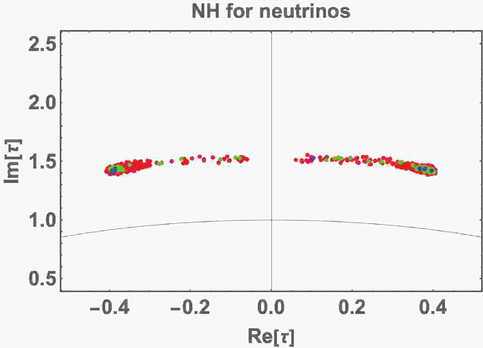
$ t_\beta\equiv v_1/v_2 $ , and$ \sqrt{v_1^2+v_2^2} = 246 $ GeV. We perform numerical analysis under the above regions. Figure 1 illustrates the correlation between the real and imaginary parts of τ, where the blue, green, and red points are allowed within 2, 3, and 5 of the$ \Delta \chi^2 $ analysis, respectively, for five accurately known observables$ \Delta m^2_{\rm{atm}},\Delta m^2_{\rm{sol}},s_{12}^2,s_{23}^2,s_{13}^2 $ in Nufit 5.0 [103, 104]. The real part runs through the entire range, but the imaginary part is localized at the$ [1.35-1.5] $ .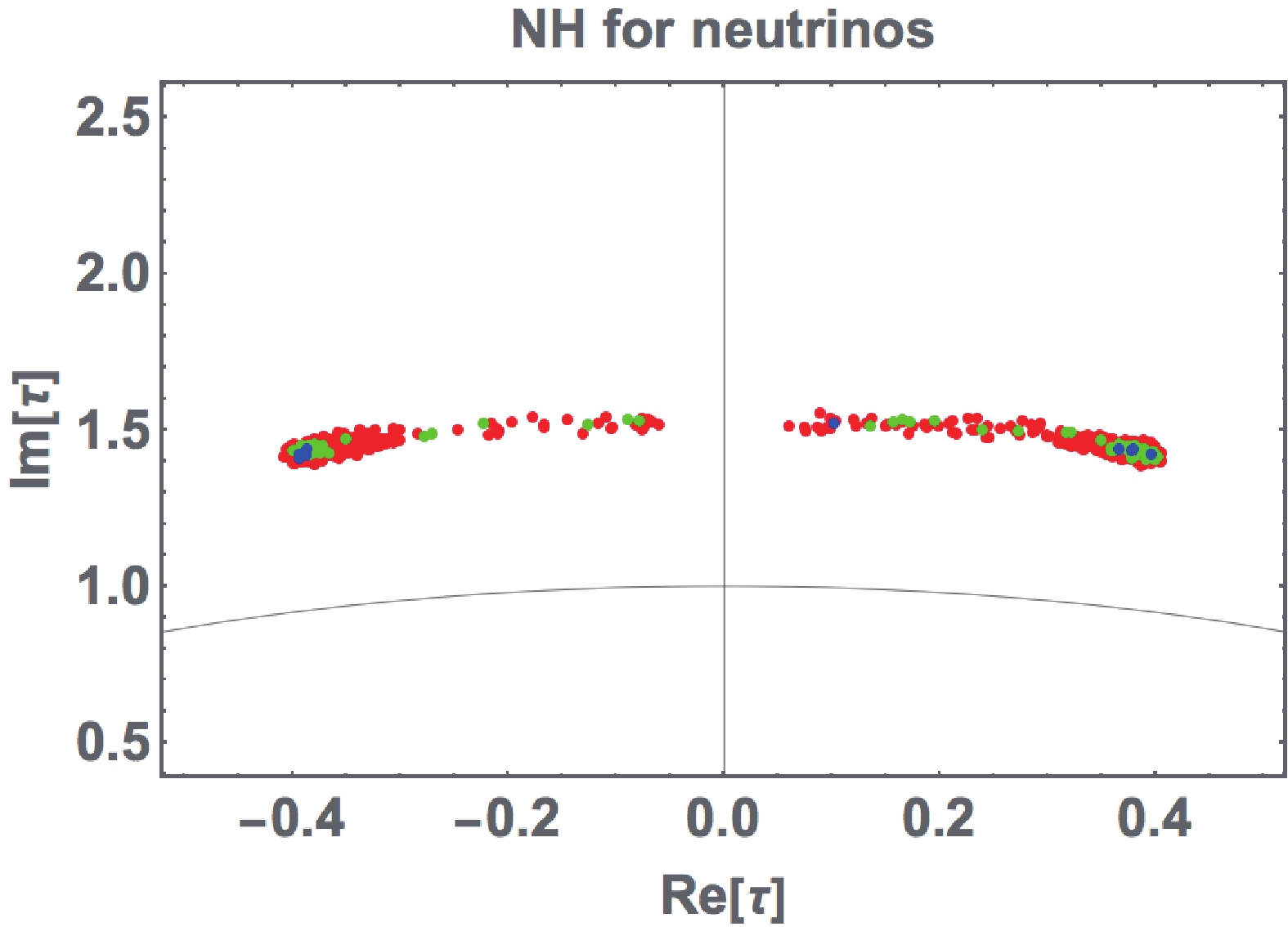
Figure 1. (color online) Allowed region of modulus τ, where the blue, green, and red points are allowed within 2, 3, and 5 of the
$ \Delta \chi^2 $ analysis, respectively.Figure 2 illustrates the correlation between the Majorana phase
$ \alpha_{21} $ and Dirac CP phase$ \delta_{\rm CP} $ . The legend is the same as in the case of Fig. 1. We identify a clear feature in the region where$ \alpha_{21} $ is within$ \{0^\circ - 120^\circ, 240^\circ - 310^\circ \} $ , while$ \delta_{\rm CP} $ is within$ \{70^\circ - 290^\circ \} $ .
Figure 2. (color online) Correlation between a Majorana phase
$ \alpha_{21} $ and$ \delta_{\rm CP} $ , where the legend is the same as the case of Fig. 1.The upper figures in Fig. 3 present the correlation between the effective mass for the neutrinoless double beta decay
$ \langle m_{ee} \rangle $ and the sum of neutrino masses$ \sum m_i $ in the [eV] unit, where the legend is the same as the case of Fig. 1. We determine that$ \langle m_{ee} \rangle $ is allowed within$ [0.001-0.004] $ eV. However,$ \sum m_i $ is restricted to be approximately$ 0.06 $ eV, which would be a sharp prediction of this model.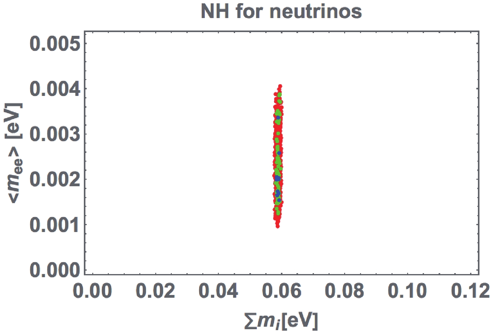
Figure 3. (color online) Predicted correlation between the effective mass for the neutrinoless double beta decay
$ \langle m_{ee} \rangle $ and the sum of neutrino masses$ \sum m_i $ in [eV], where the legend is the same as the case of Fig. 1.Finally, we present a benchmark in Table 2, which is selected, such that
$ \sqrt{\Delta \chi^2} $ is minimum. The mass matrices for the dimensionless neutrino and charged-lepton are determined asparameter valve τ $0.113762 + 1.43906 {\rm i}$ 

$ t_\beta $ 

$ 98.6 $ 

$ [\alpha_\ell, \gamma_{\ell}, \beta_{\ell}] $ 

$ [1.72\times 10^{-5},\ 6.15\times 10^{-4},\ 8.06\times 10^{-4}] $ 

$[\alpha_{\rm D}, \alpha_{NS}, \beta_{NS}]$ 

$ [-0.0112907,\ -0.00078512,\ 0.0203379] $ 

$[\beta_{\rm D}, \gamma_{\rm D}]$ 

$[-0.01432- 0.00360 {\rm i},-1.90\times 10^{-5} - 2.34\times10^{-6} {\rm i}]$ 

$ \Delta m^2_{\rm{atm}} $ 

$ 2.53\times10^{-3} {\rm{eV}}^2 $ 

$ \Delta m^2_{\rm{sol}} $ 

$ 7.48\times10^{-5} {\rm{eV}}^2 $ 

$ \sin^2\theta_{12} $ 

$ 0.289 $ 

$ \sin^2\theta_{23} $ 

$ 0.565 $ 

$ \sin^2\theta_{13} $ 

$ 0.02207 $ 

$[\delta_{\rm CP},\ \alpha_{21}]$ 

$ [248^\circ,\, 80.3^\circ] $ 

$ \sum m_i $ 

$ 58.5 $ meV

$ \langle m_{ee} \rangle $ 

$ 1.65 $ meV

$ \sqrt{\Delta\chi^2} $ 

$ 1.40 $ 

Table 2. Benchmark point of our input parameters and observables, which is selected, such that
$ \sqrt{\Delta \chi^2} $ is minimum.$ \begin{align} \tilde m_\nu& = \left[\begin{array}{ccc} 37.1331- 17.9304 {\rm i} & -16.2576 + 55.2032 {\rm i} & 35.2235+ 24.3462 {\rm i} \\ -16.2576 + 55.2032 {\rm i} &-40.0223 -38.1947 {\rm i} & -55.9229 + 44.0753 {\rm i} \\ 35.2235+ 24.3462 {\rm i} & -55.9229 + 44.0753 {\rm i} &-1.23231 + 74.8642 {\rm i} \\ \end{array}\right], \end{align} $ 
(29) $ \begin{align} M_\ell& = \left[\begin{array}{ccc} 0.00232 + 0.000467 {\rm i} & -0.00111 + 0.00314 {\rm i} & -0.00453 + 0.00274 {\rm i} \\ -0.282 + 0.102 {\rm i} & -0.0524 - 0.469 {\rm i}& 0.214 - 0.559 {\rm i} \\ 0.336 - 0.277 {\rm i} & 0.362 + 0.706 {\rm i}& -0.160 + 1.23 {\rm i} \\ \end{array}\right]. \end{align} $

(30) -
We studied a linear seesaw model with a field content as minimum as possible, introducing a modular
$ S_4 $ using$ U(1)_{B-L} $ symmetries. Owing to the rank two neutrino mass matrix, we obtained a vanishing neutrino mass eigenvalue. Furthermore, only the normal mass hierarchy of neutrinos was favored via the modular$ S_4 $ symmetry. In our numerical$ \Delta \chi^2 $ analysis, we determined a rather sharp prediction on the sum of neutrino masses to be approximately$ 60 $ meV. The imaginary part of τ was restricted at 1.35-1.5, while the real part ran through the entire range in the fundamental region. Other remarks are presented below:1.
$ \alpha_{21} $ was within$ \{0^\circ - 120^\circ, 240^\circ - 310^\circ \} $ , while$ \delta_{\rm CP} $ was within$ \{70^\circ - 290^\circ \} $ .2.
$ \langle m_{ee} \rangle $ was allowed by$ \{0.001 - 0.004\} $ eV.Therefore our model indicates several predictions in the neutrino sector that was triggered by the minimal structure with the
$ S_4 $ modular symmetry. -
This research was supported by the Korean Local Governments - Gyeongsangbuk-do Province and Pohang City (H.O.). H. O. is sincerely grateful to the KIAS member.
-
Here, we review some properties of the modular
$ S_4 $ symmetry. In general, the modular group$ \bar\Gamma $ is the group of linear fractional transformation γ acting on the modulus τ, which belongs to the upper-half complex plane and transforms as$ \begin{equation} \tau \longrightarrow \gamma\tau = \frac{a\tau + b}{c \tau + d}, \end{equation}\tag{A1} $

${\rm{where}}\; \; a,b,c,d \in \mathbb{Z}\; \; {\rm{and}}\; \; ad-bc = 1, \; \; {\rm{Im}} [\tau]>0 \; . $ This is isomorphic to
$ PSL(2,\mathbb{Z}) = SL(2,\mathbb{Z})/\{I,-I\} $ transformation. Then modular transformation is generated by two transformations S and T defined as:$ \begin{eqnarray} S:\tau \longrightarrow -\frac{1}{\tau}\ , \qquad T:\tau \longrightarrow \tau + 1\ , \end{eqnarray} \tag{A2}$

and they satisfy the following algebraic relations,
$ \begin{equation} S^2 = \mathbb{I}\ , \qquad (ST)^3 = \mathbb{I}\ . \end{equation} \tag{A3}$

Here, we introduce the series of groups
$ \Gamma(N)\; (N = $ $ 1,2,3,\dots) $ which are defined by$ \begin{align} \begin{aligned} \Gamma(N) = \left \{ \begin{pmatrix} a & b \\ c & d \end{pmatrix} \in SL(2,\mathbb{Z})\; , \; \; \begin{pmatrix} a & b \\ c & d \end{pmatrix} = \begin{pmatrix} 1 & 0 \\ 0 & 1 \end{pmatrix} \; \; ({\rm{mod}} N) \right \} \end{aligned}, \end{align}\tag{A4} $

and we define
$ \bar\Gamma(2)\equiv \Gamma(2)/\{I,-I\} $ for$ N = 2 $ . Because the element$ -I $ does not belong to the$ \Gamma(N) $ for$ N>2 $ case, we have$ \bar\Gamma(N) = \Gamma(N) $ , which are the infinite normal subgroup of$ \bar \Gamma $ known as principal congruence subgroups. Hence, we obtain finite modular groups as the quotient groups defined by$ \Gamma_N\equiv \bar \Gamma/\bar \Gamma(N) $ . For these finite groups$ \Gamma_N $ ,$ T^N = \mathbb{I} $ is imposed, and the groups$ \Gamma_N $ with$ N = 2,3,4,5 $ are isomorphic to$ S_3 $ ,$ A_4 $ ,$ S_4 $ and$ A_5 $ , respectively [11].Modular forms of level N are holomorphic functions
$ f(\tau) $ transformed under the action of$ \Gamma(N) $ , which is expressed as:$ \begin{equation} f(\gamma\tau) = (c\tau+d)^k f(\tau)\; , \; \; \gamma \in \Gamma(N)\; , \end{equation}\tag{A5} $

where k denotes the reputed modular weight.
Here, we discuss the modular symmetric theory framework without imposing supersymmetry explicitly, considering the
$ S_4 $ ($ N = 4 $ ) modular group. Under the modular transformation in Eq. (A1), a field$ \phi^{(I)} $ is also transformed as$ \begin{equation} \phi^{(I)} \to (c\tau+d)^{-k_I}\rho^{(I)}(\gamma)\phi^{(I)}, \end{equation} \tag{A6}$

where
$ -k_I $ represents the modular weight and$ \rho^{(I)}(\gamma) $ denotes a unitary representation matrix of$ \gamma\in\Gamma(4) $ . Hence, a Lagrangian such as the Yukawa terms can be invariant if the sum of modular weight from fields and the modular form in the corresponding term is zero (also invariant under$ S_4 $ and gauge symmetry).The kinetic and quadratic terms of the scalar fields can be expressed as:
$ \begin{equation} \sum\limits_I\frac{|\partial_\mu\phi^{(I)}|^2}{(-i\tau+i\bar{\tau})^{k_I}} \; , \quad \sum\limits_I\frac{|\phi^{(I)}|^2}{(-i\tau+i\bar{\tau})^{k_I}} \; , \end{equation}\tag{A7} $

which is invariant under the modular transformation, and the overall factor is eventually absorbed by a field redefinition consistently. Therefore, the Lagrangian associated with these terms should be invariant under the modular symmetry.
The basis of modular forms with weight 2,
$ Y^{(2)}_{\rm{2}} = (y_{1},y_{2}) $ and$ Y^{(2)}_{\rm{3'}} = (y_{3},y_{4},y_{5}) $ , which are transformed as a doublet and triplet under$ S_4 $ , are determined in terms of the Dedekind eta-function$ \eta(\tau) $ and its derivative [10]:$ \begin{aligned}[b] y_1(\tau) = & \frac{\rm i}{8} \left( 8 \frac{\eta'\left(\tau+\dfrac12\right)}{\eta\left(\tau+\dfrac12\right)} + 32 \frac{\eta'(4\tau)}{\eta(4\tau)} - \frac{\eta'\left(\dfrac\tau4\right)}{\eta\left(\dfrac\tau4\right)}- \frac{\eta'\left(\dfrac{\tau+1}4\right)}{\eta\left(\dfrac{\tau+1}4\right)}\right. \\&\left.- \frac{\eta'\left(\dfrac{\tau+2}4\right)}{\eta\left(\dfrac{\tau+2}4\right)} - \frac{\eta'\left(\dfrac{\tau+3}4\right)}{\eta\left(\dfrac{\tau+3}4\right)} \right), \\ y_2(\tau) = & \frac{ {\rm i} \sqrt3}{8} \left(\frac{\eta'\left(\dfrac\tau4\right)}{\eta\left(\dfrac\tau4\right)} - \frac{\eta'\left(\dfrac{\tau+1}4\right)}{\eta\left(\dfrac{\tau+1}4\right)} + \frac{\eta'\left(\dfrac{\tau+2}4\right)}{\eta\left(\dfrac{\tau+2}4\right)} - \frac{\eta'\left(\dfrac{\tau+3}4\right)}{\eta\left(\dfrac{\tau+3}4\right)} \right), \\ y_3(\tau) = & {\rm i} \left(\frac{\eta'\left(\tau+\dfrac12\right)}{\eta\left(\tau+\dfrac12\right)} - 4 \frac{\eta'(4\tau)}{\eta(4\tau)} \right), \\ y_4(\tau) = & \frac{\rm i}{4\sqrt2} \left( - \frac{\eta'\left(\dfrac\tau4\right)}{\eta\left(\dfrac\tau4\right)}+{\rm i} \frac{\eta'\left(\dfrac{\tau+1}4\right)}{\eta\left(\dfrac{\tau+1}4\right)} +\frac{\eta'\left(\dfrac{\tau+2}4\right)}{\eta\left(\dfrac{\tau+2}4\right)} - {\rm i} \frac{\eta'\left(\dfrac{\tau+3}4\right)}{\eta\left(\dfrac{\tau+3}4\right)} \right), \end{aligned}$

$ \begin{aligned}[b] y_5(\tau) = \frac{\rm i}{4\sqrt2} \left( - \frac{\eta'\left(\dfrac\tau4\right)}{\eta\left(\dfrac\tau4\right)} - i \frac{\eta'\left(\dfrac{\tau+1}4\right)}{\eta\left(\dfrac{\tau+1}4\right)} + \frac{\eta'\left(\dfrac{\tau+2}4\right)}{\eta\left(\dfrac{\tau+2}4\right)} +{\rm i} \frac{\eta'\left(\dfrac{\tau+3}4\right)}{\eta\left(\dfrac{\tau+3}4\right)} \right) . \end{aligned} \tag{A8}$

$ y_i $ 's can be expanded in terms of q as follows:$ \begin{align} y_1 & = - 3 \pi \left(\frac{b_1}{8} + 3 b_5\right),\; \ y_2 = 3 \sqrt{3} \pi b_3,\; \ y_3 = - \pi \left( -\frac{b_1}{4} + 2 b_5\right), \\ y_4 & = - \pi \sqrt{2} b_2, \;\ y_5 = - 4\pi \sqrt{2} b_4, \end{align}\tag{A9} $

where
$ b_i $ are given by$ \begin{align} b_1 \sim 1, \;\;\ b_2 \sim q,\;\; \ b_3 \sim q^2,\; \;\ b_4 \sim 0,\; \;\ b_5 \sim 0, \end{align} \tag{A10}$

with
$ q = \exp(2 \pi i \tau) $ and$ |q| \ll 1 $ [96].Subsequently, Yukawas with higher weights are constructed by the multiplication rules of
$ S_4 $ , and the following couplings can be obtained:$ \begin{aligned}[b] &Y^{(4)}_{\bf2} = \left[\begin{array}{c} y_2^2-y_1^2 \\ 2 y_1 y_2 \\ \end{array}\right], \;\;\; Y^{(4)}_{\bf3} = \left[\begin{array}{c} -2y_2y_3 \\ \sqrt3 y_1 y_5+ y_2 y_4 \\ \sqrt3 y_1 y_4+ y_2 y_5 \\ \end{array}\right],\\& Y^{(4)}_{\bf3'} = \left[\begin{array}{c} 2y_1y_3 \\ \sqrt3 y_2 y_5 - y_1 y_4 \\ \sqrt3 y_2 y_4- y_1 y_5 \\ \end{array}\right] . \end{aligned} \tag{A11}$

Linear seesaw model with a modular S4 flavor symmetry
- Received Date: 2021-12-23
- Available Online: 2022-05-15
Abstract: We discuss a linear seesaw model with a field content as minimum as possible, introducing a modular


 DownLoad: