


 Abstract
 HTML
HTML Reference
 Related
 PDF
PDF


-
The general relativity theory (GRT) is without any doubt the best theory of gravitational interaction. Although its predictions have been tested to very high precision [1], there are still open questions that make the GRT incomplete. Such questions arise at short distances and small time scales viz., black hole and cosmological singularities, respectively, for which any predictability is lost. However, the observational prediction of cosmic microwave background radiation (CMBR) and the formation of primordial light elements (Big Bang nucleosynthesis) undoubtedly represent the greatest success of GRT. Although these are fundamental results, deviations from GRT (hence from the action of Einstein-Hilbert (EH) on which GRT is based) are necessary, and new ingredients, such as dark matter and dark energy [2, 3], are needed for fitting the current picture of our Universe. In this respect, alternative or modified theories of gravity have aroused great interest. Compact stellar structures, such as quark stars, dark stars, gravastars, neutron stars, and black holes, were well-considered in various generalizations of the GRT, and astrophysical implications were contemplated that can impose restraint on these theories (for a review, see [4]). Well-accepted gravitational tests of gravity include the strong and weak field regime tests. Regarding these tests, the strong-field regime tests are considered to be more significant for analyzing the correct gravity theory. This is because in the strong-field, the gravity given by the modified theories diverts widely from that given by GRT, whereas in the weak-field, it is compatible with that given by GRT [5-11]. In this regard, scalar-tensor gravity theories as modified gravity theories have been proven to be effective in explaining several noticeable problems such as the late and early behavior of the Universe, inflation, cosmic acceleration, and coincidence problem [12-14]. Brans and Dicke [15] proposed a scalar-tensor generalization of GRT by substituting a time-modifying gravitational constant viz.,
$ G(t) = 1/{\Phi(t)} $ , and through a scalar field interaction with a geometry well-known as the Brans-Dicke (BD) gravity theory. This theory of gravity is one of the most interesting scalar-tensor theories owing to its immense cosmological implications [12-14]. Moreover, Mach's principle, agreement with the weak equivalence principle, Dirac's large number hypothesis, the varying gravitational constant, and the non-minimal coupling between the scalar field and geometry are some dominant aspects of this scalar-tensor theory [15, 16]. The authors [17, 18] used local gravity tests and showed that the general dimensionless BD-parameter$\omega_{\rm BD}$ ought to be extremely huge, i.e.,$\omega_{\rm BD} \geq 4\times 10^4$ , to be compatible with close solar system experiment bounds. The bounds on the value of the BD-parameter$\omega_{\rm BD}$ are obtained by including a massive scalar field Φ as well as a potential function$ V(\Phi) $ generated in the background of self-interacting BD theory [19]. Regarding the self-interacting BD gravity, all values of the BD-parameter$\omega_{\rm BD}$ greater than$ -3/2 $ are allowable. This theory of gravity transforms into GRT if the scalar field is constant, and the BD-parameter$\omega_{\rm BD}$ goes to infinity ($\omega_{\rm BD} \longrightarrow \infty$ ). Generally, it has been indicated [20, 21] that the BD theory is reducible to GRT only if the trace of stress-energy tensor$T^ {\rm matt}$ does not disappear, i.e.,$T^ {\rm matt} \ne 0$ .It is worth mentioning that over the past decade, several models of astrophysical objects viz., stars and galaxies, among others, have been investigated in various manners, in addition to the cosmic evolution of the Universe in the BD theory, which contributes significantly to the discovery and understanding of different relativistic phenomena. In this context, Yazadjiev et al. [22, 23] explored the dynamics of slowly and rapidly rotating compact structures, specifically neutron stars within the sight of a massive scalar field, and deduced that deviations from GRT can be large because of the moment of inertia, which is crucial. Moreover, Koyama in [24] has supposed that the Vainshtein mechanism of the Sun does not influence the scalar field profile produced by a distant compact stellar structure and showed that the scalar memory effect supplies a powerful method to test BD gravity with the Vainshtein mechanism.
For a physically viable spherical object, it is important to add some extra condition on the geometry and matter variables or offer a particular type of state equation. In an entirely different scenario, a 4-D (D
$ \equiv $ dimensional) curved space-time was implanted into a larger-D flat variety to establish various suitable stellar systems [25]. It should be noted that the n-D pseudo-Riemannian space$ V_n $ can be implanted into m-D pseudo-Euclidean variety$ V_m $ , where$ V_P $ provides an implanting class of the least number of additional P given that P must be less than$ [n-m] $ or equivalent to$ [(n^2-n)/2] $ . The implanting class of the interior Schwarzschild solution and usual FRW space-time is one, whereas the exterior entails class-two implanting. This concept of implanting gives a basic extra relation to connecting both gravitational potential components viz., radial and temporal of the space-time, named as the "Karmarkar condition" [26, 27]. We can infer the implanting class-one solution using this requirement in the background of static spherically symmetric geometry. In [28, 29], the physical plausibility of the implanting class-one anisotropic stellar configuration models was analyzed, and the compatibility of the physical parameters with the necessary stellar comportment was concluded. The same authors constructed new solutions by determining various potential candidates. They also determined the generalized form of an anisotropic stellar structure employing the Karmarkar requirement. Singh et al. [30-32] established anisotropic spherically symmetric stellar structure models with the Karmarkar condition comprising the implanting class-one solution and analyzed the outcomes via theoretical stellar configuration systems. Errehymy and his collaborators [33] implanted the curved structure into 5-D Euclidean space-time to discover the implanted class-one stellar bodies. The authors [34, 35] investigated various anisotropic stellar objects free from any physical or geometrical singularities using the Karmarkar condition.Based on the aforementioned information, the coupling functions of the BD theory with a massive scalar field, which are permitted by observation, may vary importantly from those in the massless case. This phenomenon normally leads us to conclude that the anisotropic compact stellar structures with a massive scalar field could generally have slightly extraordinary configurations and attributes compared with their homologs in the massless case. Accordingly, by taking into account this motivation, in this study, we embed a spherically symmetric static metric in Schwarzschild coordinates into a 5-D flat space for compact stellar objects in massive Brans-Dicke (MBD) gravity, to explore the possibility of providing exact solutions for viable anisotropic stellar systems through the modified Einstein field equations. The paper is organized as follows: following an exhaustive introduction in Sect. I, the appropriate BD theory under the embedding approach is laid down in Sect. II. In the same section, the basic stellar equations with the MIT bag model is constructed. In Sect. III, we provide the necessary conditions for a singularity-free matching on the boundary of the stellar configuration. In Sect. IV, we give the physical properties of the anisotropic stellar structure in MBD gravity via several physical and mathematical tests. Finally, in Sect. V, concluding remarks are reported.
-
The action of scalar-tensor theories can be addressed in two conformally linked frames namely, the Jordan and Einstein frames. In the Jordan frame, the MBD scalar field acts as a spin-zero component of gravity while it behaves as a matter source in the conformally redefined frame. The Jordan formularization results in an unstable system because of the non-positive energy density of the scalar field. However, the non-minimal coupling of the scalar field to normal matter prompts non-geodesic ways for test particles in the Einstein frame [36]. Nevertheless, the violation in the Einstein frame is trivial and the frame remains consistent with the tests of the equivalence principle. The action of MBD gravity in the Jordan frame [19] with relativistic units
$ 8\pi = G = c = 1 $ is characterized as$ S = \int\sqrt{-g}\left({\cal{R}}\Phi-\frac{\omega_{\rm BD}}{\Phi}\nabla^{\alpha}\nabla_{\alpha}\Phi -{\cal{L}}(\Phi)+{\cal{L}}_m\right) {\rm d}^{4}x, $

(1) where
$ g = |g_{\alpha\beta}| $ ,$ {\cal{R}} $ , and$ {\cal{L}}_m $ are the determinant of the metric tensor, the Ricci scalar, and the matter Lagrangian, respectively, Φ is a scalar field, and$ \omega_{BD} $ is a dimensionless BD coupling constant. Here, the function$ {\cal{L}}(\Phi) $ completely specifies the scalar-tensor theory. For the present study, we define$ {\cal{A}}(\Phi) = {\rm Exp}\left[{\frac{\Phi^2}{(2 \omega_{\rm BD}+3)^{1/2}}}\right] , {\cal{L}}(\Phi) = \frac{1}{2}m_{\Phi}^2\Phi^2 , $

(2) where
$ m_{\Phi} $ is the mass of the scalar field. For the form of scalar field function expressed in (2), the two rapidly and slowly turning NSs have effectively been investigated by Doneva et al. [37] and Yazadjiev et al. [22]. The scalar field$ \hat{\Phi} $ and metric$ \hat{g}_{\alpha\beta} $ can be obtained for the Einstein frame by means of the transformations$ \Phi = {\cal{A}}^{-2}(\hat{\Phi}) $ and$ \hat{g}_{\alpha\beta} = {\cal{A}}^{-2}(\Phi){g}_{\alpha\beta} $ . The MBD field equations and evolution equation, through the variation of action (1) with respect to$ g_{\alpha\beta} $ and Φ, are given explicitly as follows:$ \begin{aligned}[b] G_{\alpha\beta} =& R_{\alpha\beta}-\frac{1}{2}g_{\alpha\beta}R\\ =& \frac{1}{\Phi}\Bigg[T_{\alpha\beta}^{\rm (matt)}+T_{\alpha\beta}^{\Phi}\Bigg]\\ =& \frac{1}{\Phi}\Bigg[T_{\alpha\beta}^{\rm (matt)} +\Phi_{,\alpha;\beta}-g_{\alpha\beta}\Box\Phi+\frac{\omega_{\rm BD}}{\Phi} \Bigg[\Phi_{,\alpha}\Phi_{,\beta}\\ &- \frac{g_{\alpha\beta}\Phi_{,\alpha}\Phi^{,\alpha}}{2}\Bigg]-\frac{{\cal{L}}(\Phi)g_{\alpha\beta}}{2}\Bigg], \end{aligned} $

(3) $ \Box\Phi = \frac{1}{3+2\omega_{\rm BD}}\Bigg[T^{\rm (matt)}+\Phi\frac{{\rm d}{\cal{L}}(\Phi)}{{\rm d}\Phi}-2{\cal{L}}(\Phi)\Bigg],$

(4) where
$T_{\alpha\beta}^{\rm (matt)}$ describes the stress-energy tensor in the Einstein frame and$T^{\rm (matt)}$ is its trace, with$ \Box $ being the d'Alembertian operator. The stress-energy tensor in Einstein frame is linked to its conformal counterpart$ \hat{T}_{\alpha\beta} $ through$ T_{\alpha\beta} = {\cal{A}}^{2}(\Phi)\hat{T}_{\alpha\beta} $ .We suppose that the interior space-time line element for a static and spherically symmetric is represented by the following form
$ {\rm d}s^2 = {\rm e}^{\eta(r)}{\rm d}t^2-{\rm e}^{\xi(r)}{\rm d}r^2-r^2({\rm d}\theta^2+\sin^2\theta {\rm d}\phi^2), $

(5) where
$ \eta(r) $ and$ \xi(r) $ are the unknown metric potentials that have functional dependence on the radial coordinate, r, only. Heavenly systems are defined by anisotropic pressure and inhomogeneous energy density, which take a dominant part in their development. In this regard, we argue that the physical features (energy density (ρ), radial ($ p_r $ )/transverse ($ p_t $ ) pressure)) of cosmic bodies with an anisotropic distribution are specified via the following stress-energy tensor$ T_{\alpha\beta}^{\rm (matt)} = (\rho+p_t) u_{\alpha}u_{\beta}-p_t g_{\alpha\beta}+(p_r-p_t)s_{\alpha}s_{\beta}, $

(6) here
$u_\alpha = ({\rm e}^{\frac{\eta}{2}},0,0,0)$ and$s_{\beta} = (0,-{\rm e}^{\frac{\xi}{2}},0,0)$ represent the four-speed of a comoving observer and the radial four-vector, respectively. Further,$ \rho,\; p_r $ , and$ p_t $ denote the energy density, radial, and transverse pressures, respectively. Employing Eqs. (3)–(6), the field equations are acquired as$ \frac{1}{r^2}-{\rm e}^{-\xi}\left(\frac{1}{r^2}-\frac{\xi'}{r}\right) = \frac{1}{\Phi}({\rho}+T_0^{0\Phi}),$

(7) $ -\frac{1}{r^2}+{\rm e}^{-\xi}\left(\frac{1}{r^2}+\frac{\eta'}{r}\right) = \frac{1}{\Phi}({p_r}-T_1^{1\Phi}),$

(8) $ \frac{{\rm e}^{-\xi}}{4}\left(2\eta''+\eta'^2-\xi'\eta'+2\frac{\eta'-\xi'}{r}\right) = \frac{1}{\Phi}({p}_{t}-T_2^{2\Phi}),$

(9) Further, the prime symbol indicates differentiation with respect to the radial coordinate, r, and the expressions of
$ T_0^{0\Phi},\; T_1^{1\Phi} $ , and$ T_2^{2\Phi} $ are given as$ T_0^{0\Phi} = {\rm e}^{-\xi}\left[\Phi''+\left(\frac{2}{r}-\frac{\xi'}{2} \right)\Phi'+\frac{\omega_{\rm BD}}{2\Phi}\Phi'^2-{\rm e}^\xi\frac{{\cal{L}}(\Phi)} {2}\right],$

(10) $ T_1^{1\Phi} = {\rm e}^{-\xi}\left[\left(\frac{2}{r}+\frac{\eta'} {2}\right)\Phi'-\frac{\omega_{\rm BD}}{2\Phi}\Phi'^2-{\rm e}^\xi\frac{{\cal{L}}(\Phi)}{2})\right], $

(11) $ T_2^{2\Phi} = {\rm e}^{-\xi}\left[\Phi''+\left(\frac{1}{r}-\frac{\xi'} {2}+\frac{\eta'}{2}\right)\Phi'+\frac{\omega_{\rm BD}}{2\Phi}\Phi'^2-{\rm e}^\xi\frac{{\cal{L}}(\Phi)}{2} \right].$

(12) The wave equation expressed in (4) turns out to be
$ \begin{aligned}[b] \Box\Phi =& -{\rm e}^{-\xi}\left[\left(\frac{2}{r}-\frac{\xi'} {2} +\frac{\eta'}{2}\right)\Phi'(r)+\Phi''(r)\right]\\ =& \frac{1}{2}{\rm e}^{\xi}\left[\frac{{\cal{A}}^{4}(\Phi)}{\left(3+2\omega_{\rm BD}\right)^{1/2}}\left(\rho -p_r -2 p_t\right) -\frac{1}{2}\frac{{\rm d}{\cal{L}}(\Phi)}{{\rm d}\Phi}\right]. \end{aligned} $

(13) It was demonstrated that if a symmetric tensor
$ b_{\alpha\beta} $ fulfills the Gauss-Codazi equations defined as$ R_{\alpha\beta\mu\upsilon} = 2eb_{\alpha[\mu}b_{\upsilon]\beta}\quad {\rm{and}} \quad b_{\alpha[\beta;\mu]}-\alpha^{\xi}_{\beta\mu}b_{\alpha\xi} +\alpha^\xi_{\alpha[\beta}b_{\mu]\xi} = 0, $

(14) the
$ (n+1)- $ dimensional space can be incorporated in an$ (n+2)- $ dimensional pseudo-Euclidean space [38]. Further,$ b_{\alpha\beta} $ are the coefficients of second differential form and$ e = \pm1 $ ,$ R_{\alpha\beta\mu\upsilon} $ indicates the curvature tensor. From the relationship expressed in (14), a necessary and sufficient condition for a class-one embedding was obtained by Eiesland [39] as follows$ R_{0101}R_{2323}-R_{1212}R_{0303}-R_{1202}R_{1303} = 0, $

(15) which prompts the accompanying differential equation for the considered metric gravitational potential
$ (\xi'-\eta')\eta'e^\xi+2(1-e^\xi)\eta''+\eta'^2 = 0. $

(16) The solution corresponding to the equation expressed in (16) turns out to be
$ \xi(r) = \ln(1+D\eta'^2e^\eta), $

(17) where D is an integration constant. To solve the stellar system of field equations, we choose
$ g_{tt} $ component of the space-time as$ \eta(r) = 4\ln \left(B^{1/4}(1+Ar^2)\right), $

(18) where A and B are positive constants. Using this gravitational potential
$ \eta(r) $ in Eq. (17), we obtain$ \xi(r) = \ln(1+ACr^2(1+Ar^2)^{2}), $

(19) where
$ C = 64ABD $ is a constant.NSs with
$ M>3M_{\bigodot} $ might turn into QSs which hold up$ (u) $ , down$ (d) $ , and strange$ (s) $ quark flavors. In this context, the matter variables viz., density and pressure representing the interior configuration of these relativistic stars, obey the Massachusetts Institute of Technology (MIT) bag equation of state (EoS). Moreover, we suppose that non-interacting and massless quarks occur within the stellar geometries. According to the MIT bag model, the quark pressure$ p_r $ may be cast as$ p_r = \sum\limits_{f}p^f-{\cal{B}},\quad f = u,\; d,\; s, $

(20) where
$ p^f $ represents the individual pressure of each quark flavor which is neutralized by the bag constant$ {\cal{B_g}} $ , also known as total external bag pressure. The total energy density of the deconfined quarks is stated by the MIT bag model as$ \rho = \sum\limits_{f}\rho^f+{\cal{B}}, $

(21) where the matter density of each flavor
$ \rho^f $ is connected to the corresponding pressure as$ \rho^f = 3p^f $ . The simplified MIT bag EoS for strange stars is concluded from Eqs. (20) and (21) as$ p_r = \frac{1}{3}(\rho-4{\cal{B}}). $

(22) It is noteworthy that this simplified form of EoS was applied with pure GR and modified gravity theories to describe the stellar systems made of the strange quark matter distribution. In the current study, the numerical solutions of the stellar system were obtained by setting
$ {\cal{B}} $ equal to$75.007\;\rm MeV/fm^3$ , which is within the allowed range [40]. The overall mass of the uncharged fluid sphere is determined via the Misner-Sharp formula as$ m = \frac{r}{2}(1-g^{\alpha\beta}r_{,\alpha}r_{,\beta}). $

(23) -
The set of parameters viz., A, B, C, D representing the geometry as well as physical properties (for example mass and radius) of anisotropic compact stellar configurations may be settled across the smooth matching of inner and outer spacetimes at the pressure-free boundary (Σ). The outer spacetime is considered to be the Schwarzschild spacetime given by,
$ {\rm d}s^2 = \left(1-\frac{2M}{r}\right){\rm d}t^2-\frac{1}{\left(1-\dfrac{2M}{r}\right)}{\rm d}r^2 -r^2({\rm d}\theta^2+\sin^2\theta {\rm d}\phi^2), $

(24) where M denotes the total mass. To corroborate continuity and smoothness of geometry at the surface layers of the star, the following conditions should be fulfilled at the pressure-free boundary Σ
$ (f = r-R = 0 $ , where R is the constant radius)$\begin{aligned}[b] ({\rm d}s^2_-)_{\Sigma} =& ({\rm d}s^2_+)_{\Sigma},\\ (K_{ij_-})_{\Sigma} = &(K_{ij_+})_{\Sigma},\end{aligned}$

(25) $ \begin{aligned}[b]&(\Phi(r)_-)_{\Sigma} = (\Phi(r)_+)_{\Sigma},\\&(\Phi'(r)_-)_{\Sigma} = (\Phi'(r)_+)_{\Sigma}.\end{aligned}$

(26) Here,
$ K_{ij} $ means curvature while subscripts - and + denote the interior and exterior spacetimes, respectively. The continuity of the first fundamental form viz.,$[{\rm d}s^2]_\Sigma = 0$ gives us$ [F]_\Sigma\equiv F(r\rightarrow R^+)-F(r\rightarrow R^-)\equiv F^+_R-F_R^-, $

(27) for any function
$ F(r) $ . This fundamental condition gives us$ g_{tt}^-(R) = g_{tt}^+(R) $ and$ g_{rr}^-(R) = g_{rr}^+(R) $ . In addition, the continuity of the second fundamental form ($ K_{ij} $ ) is equivalent to the O'Brien and Synge [41] matching conditions, stated as$ [G_{\alpha\beta}r^\beta]_\Sigma = 0, $

(28) where
$ r_\alpha $ denotes a unit radial vector. Using the field equations (7)–(9) along with the Eq. (28) inferred$ [T_{\alpha\beta}r^\beta]_\Sigma = 0 $ which says that radial pressure becomes zero at the boundary surface, i.e.,$ p_r(R) = 0 $ . Also, the scalar field relating to the vacuum Schwarzschild solution is determined utilizing the strategy in [42], and it becomes$\Phi = {\rm e}^{(1-\frac{2M}{r})}$ . We indicate the inner and outer zones by$ \Sigma^- $ and$ \Sigma^+ $ , respectively.The hypersurface is characterized by the line element
$ {\rm d}s^2 = {\rm d}\tau^2-R^2({\rm d}\theta^2+\sin^2\theta {\rm d}\phi^2), $

(29) here τ describes the proper time on the stellar surface. Furthermore, the extrinsic curvature of Σ is defined by
$ K_{ij}^{\pm} = -n_\alpha^{\pm}\frac{\partial^2x^\alpha_{\pm}}{\partial\eta^i\eta^j} -n_\alpha^{\pm}\alpha^\alpha_{\beta\mu}\frac{\partial x^\beta_{\pm}}{\partial\eta^i} \frac{\partial x^\mu_{\pm}}{\partial\eta^j}, $

(30) where the coordinates on the Σ are defined by
$ \eta^i $ . In addition, the components of the 4-vector normal to the hypersurface viz.,$ n_{\alpha}^\pm $ are defined in the coordinates i.e.,$ x^\alpha_{\pm} $ of$ \Sigma^\pm $ as$ n_{\alpha}^\pm = \pm \frac{{\rm d}f}{{\rm d} x^\alpha}\Big|g^{\beta\mu}\frac{{\rm d}f}{{\rm d}x^\beta}\frac{{\rm d}f}{{\rm d}x^\mu}\Big|^{\frac{-1}{2}}, $

(31) with
$ n_\alpha n^\alpha = 1 $ . The unit normal vectors have the following explicit form$ n^-_\alpha = (0,{\rm e}^{\frac{\xi}{2}},0,0),\quad n^+_\alpha = \left(0,\left(1-\frac{2M}{r}\right)^{\frac{-1}{2}},0,0\right). $

(32) Regarding this, comparing the metrics (5) and (24) with (29), it is easy to verify that
$ \left[\frac{{\rm d}t}{{\rm d}\tau}\right]_\Sigma = [{\rm e}^{\frac{-\eta}{2}}]_\Sigma = \left[\left(1-\frac{2M}{r}\right)^{\frac{-1}{2}}\right]_\Sigma,\quad [r]_\Sigma = R. $

(33) Employing Eq. (32), the non-zero components of curvature are determined as
$ K_{00}^- = \left[-\frac{{\rm e}^{-\frac{\xi}{2}}\eta'}{2}\right]_\Sigma, $

(34) $ K_{22}^- = \frac{1}{\sin^2(\theta)}K_{33}^- = [r {\rm e}^{-\frac{\xi}{2}}]_\Sigma, $

(35) $ K_{00}^+ = \left[-\frac{M}{r^2}\left(1-\frac{2M}{r}\right)^{\frac{-1}{2}}\right]_\Sigma, $

(36) $ K_{22}^+ = \frac{1}{\sin^2(\theta)}K_{33}^+ = \left[r\left(1-\frac{2M}{r}\right)^{\frac{1}{2}}\right]_\Sigma.$

(37) The junction conditions
$ [K^-_{22}]_\Sigma = [K^+_{22}]_\Sigma $ and$ [r]_\Sigma = R $ give$ {\rm e}^{-\frac{\xi(R)}{2}} = \left(1-\frac{2M}{R}\right)^{\frac{1}{2}}. $

(38) Substituting this last equation in the matching condition
$ [K^-_{00}]_\Sigma = [K^+_{00}]_\Sigma $ leads to$ \eta'(R) = \frac{2M}{R(R-2M)}. $

(39) Thus, the junction conditions expressed in Eqs. (33)–(39) supply the relations at the hypersurface in the following forms
$ {\rm e}^{\eta(R)} = B(AR^2+1)^4 = 1-\frac{2M}{R}, $

(40) $ {\rm e}^{-\xi(R)} = \frac{1}{1+ACR^2(AR^2+1)} = 1-\frac{2M}{R}, $

(41) $ \eta'(R) {\rm e}^{\eta(R)} = 8ABR(AR^2+1)^3 = \frac{2M}{R^2}. $

(42) The unknown parameters of the stellar system viz., A, B, C, D are determined by considering
$ C = 64ABD $ in the above equations, which are expressed in the following forms$ A = \frac{M}{R^2(4R-9M)}, $

(43) $ B = \frac{1}{R}(R-2M)\left(\frac{8M-4R}{9M-4R}\right)^{-4}, $

(44) $ C = 2\left(\frac{8M-4R}{9M-4R}\right)^{-3}, $

(45) $ D = \frac{R^3}{2M}.$

(46) To fix the arbitrariness of the unknown parameters, we contrast our solutions with the observational constraints from some measurements of the millisecond pulsars and their corresponding mass-radius ratio. For the gravitational potential functions expressed in Eqs. (18) and (19) along with Eqs. (43)–(46), the state variables viz., energy density and pressure components, are expressed in terms of total mass M and constant radius R as follows:
$\begin{aligned}[b] \rho =& \frac{12rf_{1}f_{2}}{\dfrac{f_{2}f_{3}(9MR^2-Mr^2-4R^3)^3}{16MR^2(2M-R)}+2r^2f_{5}}\\& + \frac{27Mrf_{1}}{f_{5}}+ {\cal{B}} - 6rf_{1}\Phi'^2(r) , \end{aligned} $

(47) $\begin{aligned}[b] p_r =& \frac{4rf_{1}f_{4}}{\dfrac{f_{2}f_{3}(9MR^2-Mr^2-4R^3)^3}{16MR^2(2M-R)}+2r^2f_{5}}\\& + \frac{9Mrf_{1}}{f_{5}}- {\cal{B}} - 2rf_{1}\Phi'^2(r), \end{aligned} $

(48) $ \begin{aligned}[b] p_t =& -4 r^2f_{1}{\cal{B}}{\cal{A}}^4(\Phi)\left( 1- \frac{32MR^2r^2(2M-R)}{f_{2}f_{3}f^{2}_{5}} \right) \\ & - \frac{128MR^2r^2(2M-R)}{f_{2}f_{3}f^{2}_{5}} - \frac{12Mr^2}{f_{5}} + 6f_{1}r^2\Phi'^2(r) \\ & - 2 f_{1} + \frac{2f_{3}f_{4}\left(9M(r^2-R^2)+ 4R^3\right)}{f_{3}f^{2}_{5}-32MR^2r^2(2M-R)f^{-1}_{2}}, \end{aligned} $

(49) where
$f_{1} = \Bigg[-4 r{\cal{A}}^4(\Phi)\left( 1+ \left(\frac{2Mr^2(9M-4R)}{4R^2(2M-R)(4R-9M)} \right)^3\right)\Bigg]^{-1}, $

$f_{2} = \left(1+Mr^2(R^2(4R-9M))^{-1} \right)^{-4}, $

$f_{3} = \left(1-M(9M-4R)^{-1} \right)^4, $

$f_{4} = 3Mr^2-9MR^2+4R^3, $

$f_{5} = M(r^2-9R^2)+4R^3 . $

It is worth mentioning here that we are able to analyze the salient physical characteristics of our stellar system. In the next section, we will discuss these physical features of compact stellar configurations.
-
The physical properties of strange stars can now be analyzed in the presence of a massive scalar field along with the coupling parameter across the energy density and radial/transverse pressure components. For this purpose, we have chosen the mass of the scalar field as
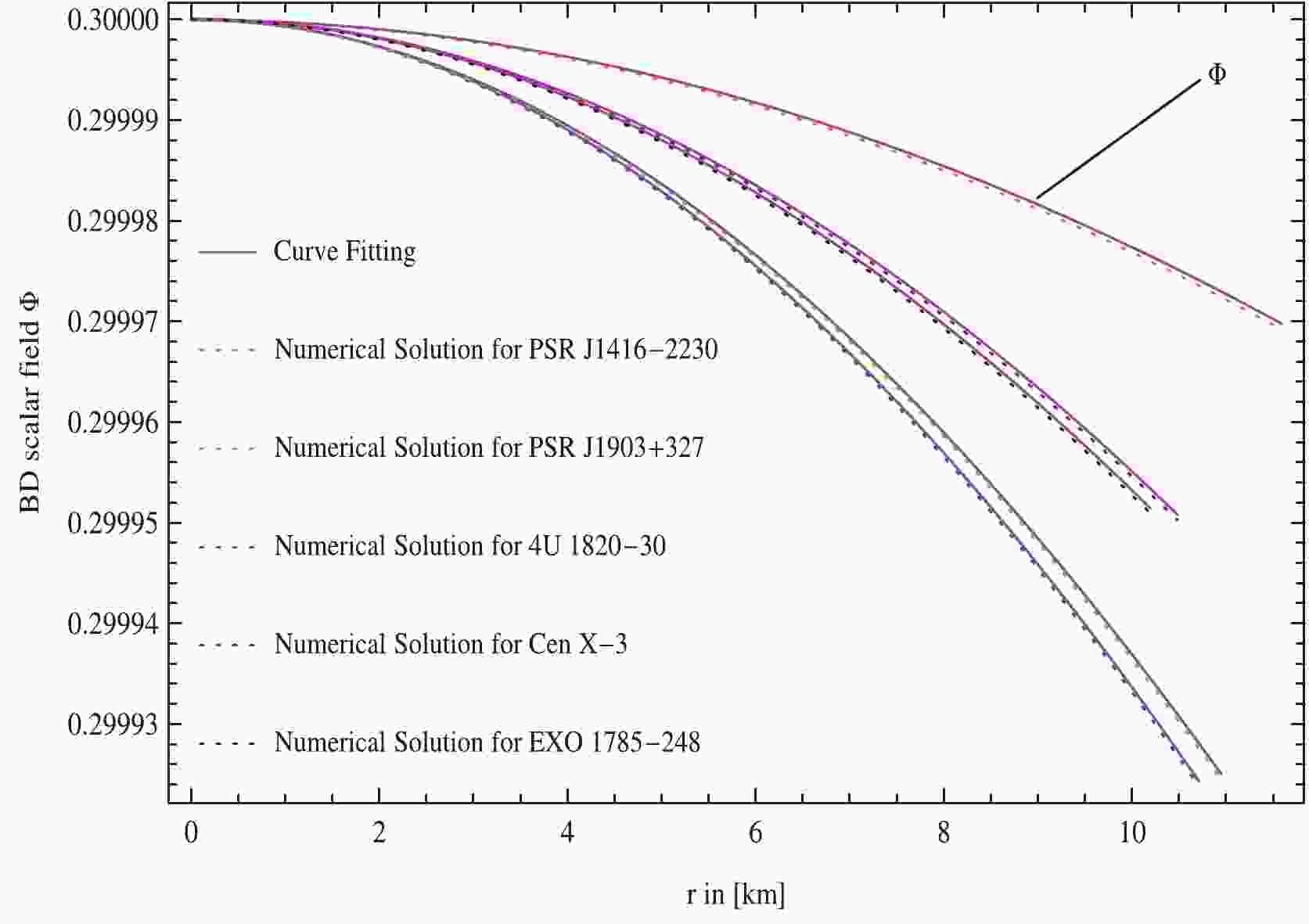
$ m_\Phi = 0.3 $ , which is well-compatible with the restraint imposed by the Gravity Probe B experiment that supplies the lower bound on the mass of scalar field, such as$ m_\Phi>10^{-4} $ in dimensionless units [37, 43]. Numerical stellar solutions have been obtained for$\omega_{\rm BD} = 05,\; $ $ 10,\; 15,\; 20,\; 25,\; 50$ which are in agreement with the restraints imposed by the solar system observations [43]. The massive scalar field is determined by solving the wave equation (13) numerically with the initial conditions$ \Phi(0) = \Phi_c = $ constant and$ \Phi'(0) = 0 $ . In this regard, the numerical solution of the wave equation (13) is well fitted (see Fig. 13) with the analytic solution given by Bruckman and Kazes [42] by relying upon the relationship between Φ and$ g_{tt} $ for static spherically symmetric space-time, as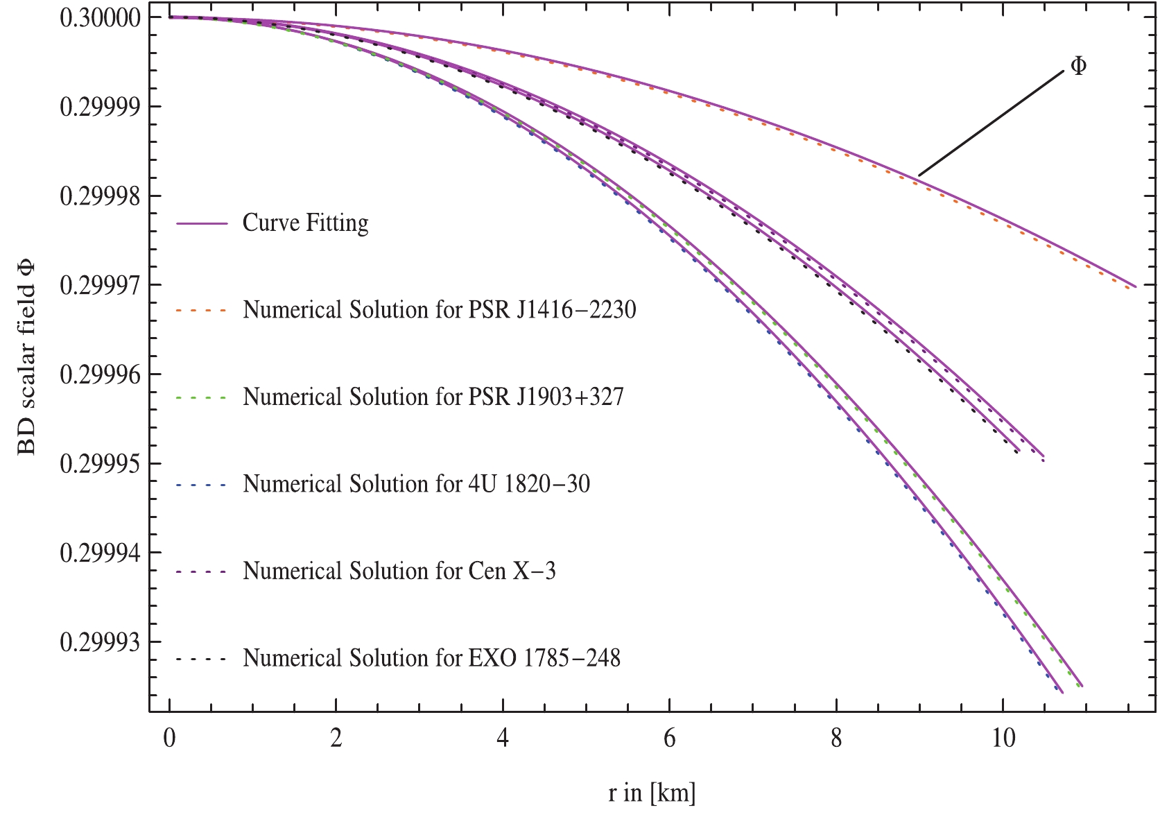
Figure 13. (color online) The scalar field
$\Phi(r)$ is plotted against radial coordinate, r, by taking the values of a, b, A, and B as shown in Table 3 for five strange stars viz., PSR J1416-2230, PSR J1903+327, 4U 1820-30, Cen X-3, and EXO 1785-248.$ \Phi(r) = a{\rm Exp}[b\eta(r)], $

(50) where a and b are two arbitrary constants. In this scenario, Maurya and his colleagues [44] were the first explorers who applied this functional form of the scalar field Φ to find precise answers to charged compact astrophysical objects by investigating new spherically symmetrical solutions of Einstein’s field equations in the background of BD gravity. In the same theory, the authors [45] have explored the existence of a new family of uncharged compact stellar configuration solutions by employing the same functional form of the scalar field Φ for an anisotropic source of fluid. The values of a and b coming from the functional form of the scalar field expressed in (50) depend on the boundary conditions imposed on the scalar field Φ, viz.,
$ \Phi(0) = \Phi_c $ ,$ \Phi'(0) = 0 $ , which are represented in Table 3 to find out the physical parameters of the compact stellar configurations. The constant$ \Phi_c $ with respect to the selected values of the parameters$m_{\Phi},\; \omega_{\rm BD}$ , and$ {\cal{B}} $ are presented in Table 1. The subscripts c and s denote that the quantity has been computed at the center and surface of the stellar configuration, respectively. All forthcoming stellar results have been illustrated graphically for U 1820-30 ($M = $ $ 1.58\pm0.06M_{\bigodot}$ [46]).Strange stars a b A B C D PSR J1416-2230 0.29990070 –0.00059001 0.000324163 0.570736 1.70428 575.734 PSR J1903+327 0.29984981 -0.00058022 0.000947973 0.421993 1.53837 240.347 4U 1820-30 0.29985855 –0.00067321 0.000856794 0.496212 1.62754 239.259 Cen X-3 0.29989402 –0.00057885 0.000668899 0.542872 1.67689 288.619 EXO 1785-248 0.29990301 –0.00057609 0.000700616 0.570341 1.70390 266.507 Table 3. Derived values of constants due to the different strange star candidates for
$m_{\phi}=0.3$ ,${\phi}_c=0.3\; \omega_{\rm BD}=20$ and${\cal{B}}= $ $ 75.007\;\rm MeV/fm^3$ .Values of $\omega_{\rm BD}$ 

Values of $\phi_c$ 

Predicted radius $\rm /Km$ 

${\rho}^{\rm eff}_c /\rm (gm/{cm}^3)$ 

${\rho}^{\rm eff}_s/\rm (gm/{cm}^3)$ 

$p_c /\rm (dyne/{cm}^2)$ 

$\dfrac{2M}{R}$ 

$Z_s$ 

05 0.281 $8.458 ^{+0.271}_{-0.290}$ 

$3.92059 \times 10^{14}$ 

$3.16144 \times 10^{14}$ 

$7.05291 \times 10^{34}$ 

0.267014 0.180115 10 0.298 $9.701 ^{+0.272}_{-0.281}$ 

3.9855 $\times 10^{14}$ 

3.20731 $\times 10^{14}$ 

$7.3361 \times 10^{34}$ 

0.325797 0.239089 15 0.312 $10.059 ^{+0.253}_{-0.273}$ 

4.0186 $\times 10^{14}$ 

3.23069 $\times 10^{14}$ 

$7.48043 \times 10^{34}$ 

0.342399 0.257771 20 0.324 $10.424 ^{+0.245}_{-0.262}$ 

4.03955 $\times 10^{14}$ 

3.24549 $\times 10^{14}$ 

$7.57179 \times 10^{34}$ 

0.359097 0.277615 25 0.337 $10.972 ^{+0.231}_{-0.250}$ 

4.05434 $\times 10^{14}$ 

3.25595 $\times 10^{14}$ 

$7.6363 \times 10^{34}$ 

0.383656 0.308943 50 0.351 $11.381 ^{+0.223}_{-0.235}$ 

4.09264 $\times 10^{14}$ 

3.28301 $\times 10^{14}$ 

$7.80339 \times 10^{34}$ 

0.401531 0.333542 Table 1. Physical parameters of
$4U~1820-30$ with$m_{\phi}$ and${\cal{B}}=75.007 \;\rm MeV/fm^3$ for different values of$\omega_{\rm BD}$ . -
For a physically valid stellar solution, the gravitational potential functions should be positive and well-comported everywhere inside the stellar configurations to guarantee a singularity-free geometry [47]. The metric potentials are displayed in Fig. 1, which reveal that both gravitational potential functions are positive, regular and monotonically increasing functions of the radial coordinate leading to a singularity free system.
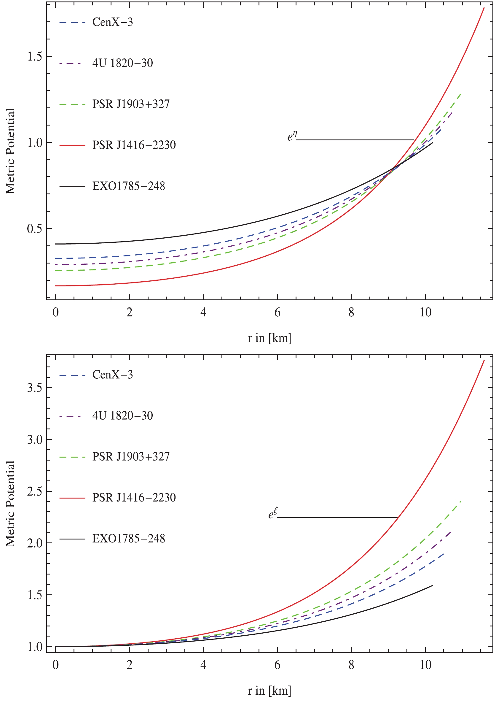
Figure 1. (color online) Evolution of metric potentials viz.,
${\rm e}^{\xi}$ and${\rm e}^{\eta}$ vs. radial coordinates r for different experimental statistics of compact stars. -
The physical variables such as energy density and pressure play an important role in determining the comportment of highly dense strange stellar configurations. The comportment of these matter variables against the radial coordinate should be positive and decrease monotonically towards the stellar surface. Figs. 2 and 3 reveal that the state determinants are maximum at the center which exhibits that the core of compact configuration is highly concentrated and decrease away from it for the selected values of the parameters
$ m_\Phi $ ,$\omega_{\rm BD}$ , and$ {\cal{B}} $ . Hence, for the chosen values of the bag constant viz.,$ {\cal{B}} $ , the existence of quark stellar structures is guaranteed for$ {\cal{L}}(\Phi) = $ $ \dfrac{1}{2}m_{\Phi}^2\Phi^2 $ .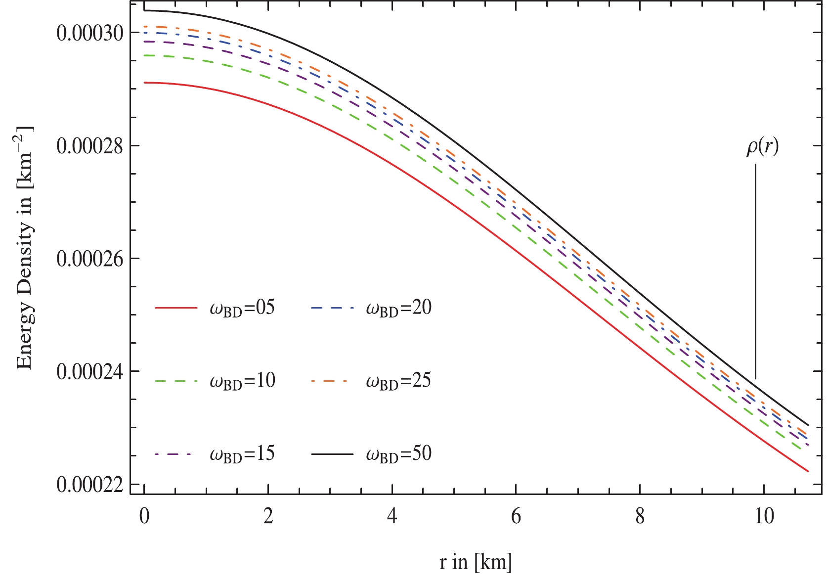
Figure 2. (color online) The matter density for 4U 1820-30 plotted against radial coordinate, r by taking
$\Phi_c = 0.3,\; m_\phi = $ $ 0.3, \; {\cal{B}} = 75.007\;\rm MeV/fm^3$ with different values of$\omega_{\rm BD}$ .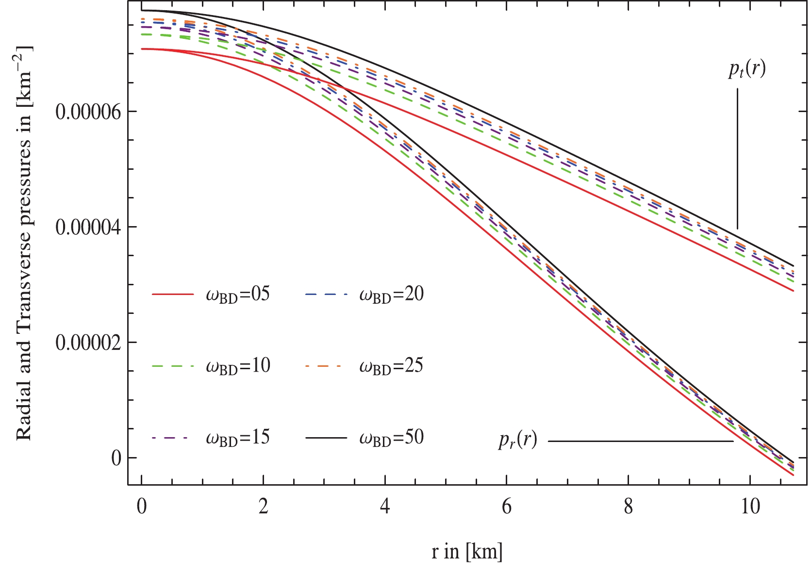
Figure 3. (color online) The radial/transverse pressure for 4U 1820-30 plotted against radial coordinate, r by taking
$\Phi_c = 0.3, $ $ m_\phi = 0.3,\; {\cal{B}} = 75.007\;\rm MeV/fm^3$ with different values of$\omega_{\rm BD}$ . -
The presence of radial and tangential components of pressure leads to anisotropy inside the stellar system. The pressure anisotropy, measured as
$ \Delta = p_t-p_r $ , is positive when the transverse pressure exceeds the radial pressure i.e.,$ p_t>p_r $ or$ \Delta>0 $ and negative otherwise, i.e., when$ p_t<p_r $ or$ \Delta<0 $ . In addition, the particles are tightly clustered jointly in dense stellar configurations which restricts the particles' motion in the radial direction. Therefore, the radial force or pressure is less than the transverse force prompting a positive anisotropy. Along these lines, the positive anisotropy produces an outward repulsive force increasing the stability and compactness of the stellar configurations stabilizing the system against gravity. Using Eqs. (48) and (49), we obtain the anisotropy in the following form$ \begin{aligned}[b] \Delta =& \frac{1}{{\cal{A}}^4(\Phi)\left(f_{3}f^{2}_{5} - 32MR^2r^2(2M-R)f^{2}_{1}\right)^2}\\ & \times \Big[4M^2r^2(-f_{3}f_{5}-8R^2(2M-R)f^{2}_{1})(-2f_{3}f^{2}_{5} \\& - 32R^2 (2M-R)f^{2}_{1} + 2f_{3}f^{2}_{5}\Phi'^2(r)(f_{3}f^{2}_{5} \\& - 32MR^2r^2(2M-R)f^{2}_{1}))\Big]. \end{aligned} $

(51) The anisotropy of the current stellar configuration, shown in Fig. 4, is positive throughout the stellar region for the chosen values of the parameters
$ m_\Phi $ ,$\omega_{\rm BD}$ , and$ {\cal{B}} $ , confirming that the selected stellar model is viable.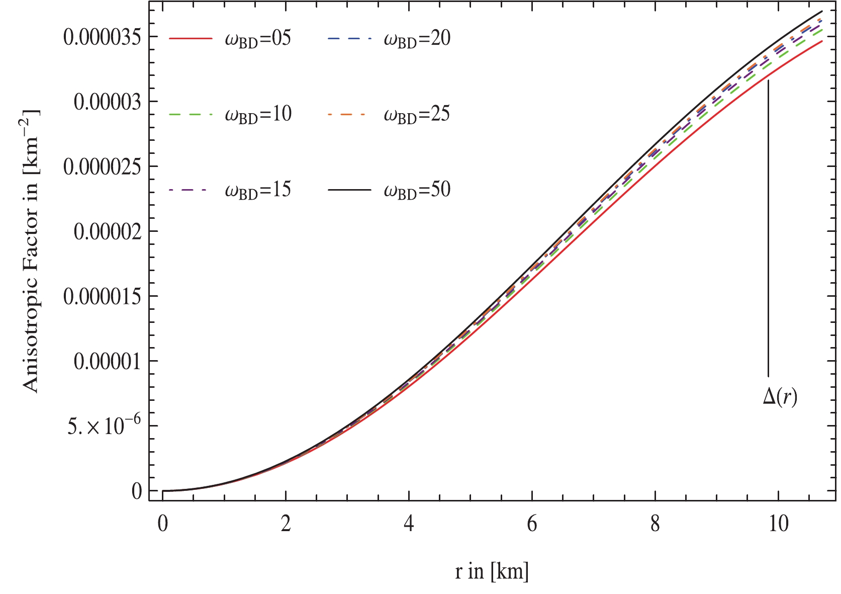
Figure 4. (color online) The anisotropy factor for 4U 1820-30 plotted against radial coordinate, r by taking
$\Phi_c = 0.3,\; m_\phi = $ $ 0.3,\; {\cal{B}} = 75.007\;\rm MeV/fm^3$ with different values of$\omega_{\rm BD}$ . -
The anisotropic configuration is said to be realistic or physically feasible if it complies with five energy conditions, i.e., null (NEC), weak (WEC), strong (SEC), dominant (DEC), and trace (TEC). In the arena of MBD gravity, these five constraints are evaluated in terms of following inequalities [48].
$ {\rm{NEC:}}\quad\rho\geq0,$

(52) $ {\rm{WEC:}}\quad\rho+p_r\geq0,\quad\rho+p_t\geq0,$

(53) $ {\rm{SEC:}}\quad\rho+p_r+2p_t\geq0,$

(54) $ {\rm{DEC:}}\quad\rho-p_r\geq0,\quad \rho-p_t\geq0,$

(55) $ {\rm{TEC:}}\quad\rho-p_r-2p_t\geq0.$

(56) The positive behavior of state determinants viz.,
$ \rho,\; p_r $ , and$ p_\perp $ displayed in Fig. 5 readily complies with the first three inequalities i.e., NEC, WEC, and SEC. The graphs corresponding to DEC and TEC in Fig. 5 exhibit that DEC and TEC are positive at each point throughout the stellar configuration. Consequently, all energy bounds are fulfilled which confirm the stellar system for the considered values of$ m_\Phi,\; {\cal{B}} $ , and$\omega_{\rm BD}$ .
Figure 5. (color online) The energy conditions for 4U 1820-30 plotted against radial coordinate, r by taking
$\Phi_c = 0.3,\; m_\phi = $ $ 0.3,\; {\cal{B}} = 75.007\;\rm MeV/fm^3$ with different values of$\omega_{\rm BD}$ . -
Size and gravitational mass are two inter-related observable features that establish the structure and compactness of compact stellar configurations. The effective mass of a stellar configuration is measured in terms of radius across Misner-Sharp definition as
$ \begin{aligned}[b] m(r) =& \frac{1}{2}r\Bigg[1-R^2\left(4R-9M\right)\Big[8Mr^2\left(1-\frac{M}{(9M-4R)}\right)^{-3}\\& \times \left(1+\frac{Mr^2}{R^2(4R-9M)}\right)^{2}+R^2(4R-9M)\Big]^{-1}\Bigg], \end{aligned} $

(57) which is subject to the radius of stellar configuration. Fig. 6 show that the gravitational mass is a monotonically increasing function with the radial coordinate and positive throughout the stellar configuration. In addition, the regularity at the center of the celestial body is confirmed for all chosen values of the parameters
$ m_\Phi,\; {\cal{B}} $ , and$\omega_{\rm BD}$ . The compactness function is the ratio of mass to radius given as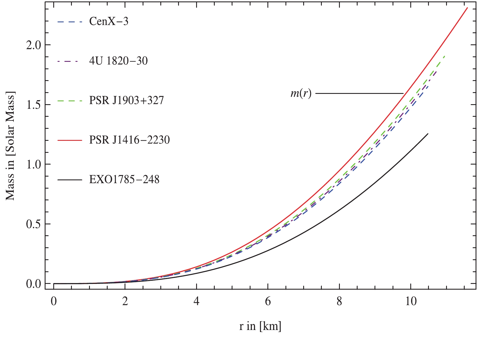
Figure 6. (color online) The mass function is plotted against radial coordinate, r for different experimental statistics of compact stars.
$ \begin{aligned}[b] u(r) =& \frac{m(r)}{r} = \frac{1}{2}\Bigg[1-R^2\left(4R-9M\right)\Big[8Mr^2\left(1-\frac{M}{(9M-4R)}\right)^{-3}\\ & \times \left(1+\frac{Mr^2}{R^2(4R-9M)}\right)^{2}+R^2(4R-9M)\Big]^{-1}\Bigg], \end{aligned} $

(58) which must be less than 0.444 as proposed by Buchdal [49] to ensure the stability of a compact cosmic body. The maximum value of the compactness function at the stellar surface is shown in Tables 1 and 2. In Fig. 7, we show that the anisotropic stellar model satisfies the required criterion i.e., adheres to the upper limit
$ \dfrac{m}{R}<\dfrac{4}{9} $ , suggested by Buchdal [49] for all chosen values of$ m_\Phi,\; {\cal{B}} $ , and$\omega_{\rm BD}$ . Moreover, under the effect of the gravitational field of a cosmic body, the electromagnetic radiation forfeits part of its energy via an increase in its wavelength, i.e., the radiation is red-shifted. The influence of the gravitational force can be measured from the X-ray spectrum of the stellar configuration utilizing the compactness factor through a gravitational red-shift parameter indicated asStrange stars Observed mass $/M_{\odot}$ 

Predicted radius /km ${\rho}^{\rm eff}_c/\rm (gm/{cm}^3)$ 

${\rho}^{\rm eff}_s /\rm (gm/{cm}^3)$ 

$p_c /\rm (dyne/{cm}^2)$ 

$\dfrac{2M}{R} $ 

$Z_s$ 

PSR J1416-2230 1.908±0.04[57] $11.589^{+0.241}_{-0.262}$ 

$4.41585 \times 10^{14}$ 

$3.35559 \times 10^{14}$ 

$4.65545 \times 10^{34}$ 

0.315046 0.238527 PSR J1903+327 1.667 ±0.021[58] $10.948^{+0.042}_{-0.053}$ 

4.02739 $\times 10^{14}$ 

3.18909 $\times 10^{14}$ 

6.22257 $\times 10^{34}$ 

0.303465 0.225854 4U 1820-30 1.58 ±0.06[59] $10.713^{+0.123}_{-0.134}$ 

3.92059 $\times 10^{14}$ 

3.13871 $\times 10^{14}$ 

7.05291 $\times 10^{34}$ 

0.297835 0.219853 Cen X-3 1.49 ±0.08[60] $10.483^{+0.171}_{-0.180}$ 

3.81935 $\times 10^{14}$ 

3.08859 $\times 10^{14}$ 

8.05473 $\times 10^{34}$ 

0.291452 0.213172 EXO 1785-248 1.3 ±0.2[61] $10.195^{+0.475}_{-0.535}$ 

3.62795 $\times 10^{14}$ 

2.98667 $\times 10^{14}$ 

1.07471 $\times 10^{35}$ 

0.276186 0.197693 Table 2. Physical parameters of the observed strange stars for
$m_{\phi}=0.3$ ,${\phi}_c=0.3$ ,$\omega_{\rm BD}=15$ , and${\cal{B}}=70\;\rm MeV/fm^3$ .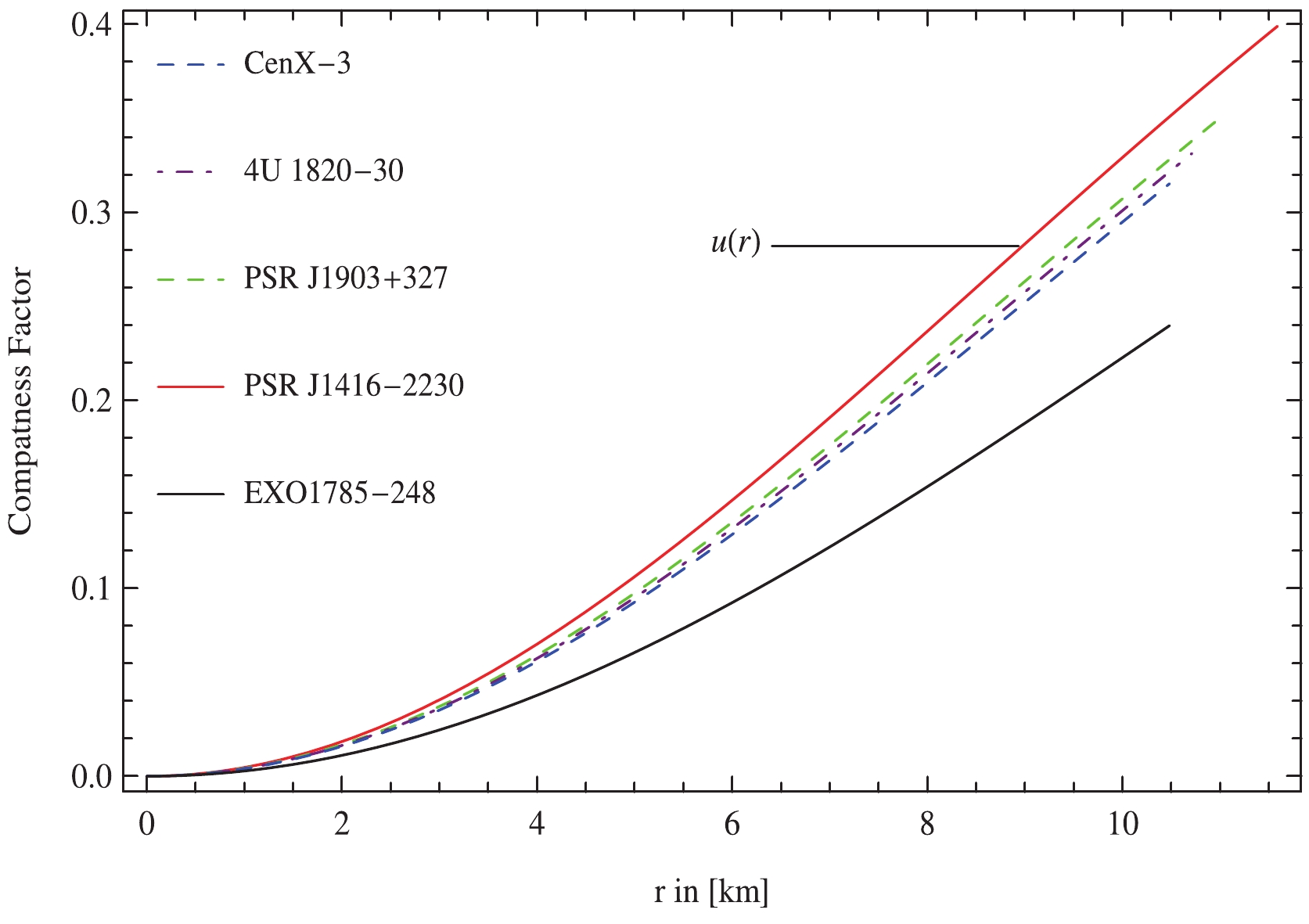
Figure 7. (color online) The compactness function is plotted against radial coordinate, r for different experimental statistics of compact stars.
$ Z = \frac{1}{\sqrt{1-2u(r)}}-1, $

(59) leading to the following explicit form
$ \begin{aligned}[b] Z =& \Bigg[R^2\left(4R-9M\right)\\ & \times \Big[R^2(4R-9M) + 8Mr^2\left(1-\frac{M}{(9M-4R)}\right)^{-3}\\ & \times \left(1+\frac{Mr^2}{R^2(4R-9M)}\right)^{2}\Big]^{-1}\Bigg]^{-1/2}-1. \end{aligned} $

(60) Figure 8 demonstrates the gravitational red-shift as an increasing function with respect to radial coordinate. Notably, the surface red-shift for the celestial candidate is in good agreement with the limit for relativistic cosmic objects viz.,
$ Z<5.211 $ [50].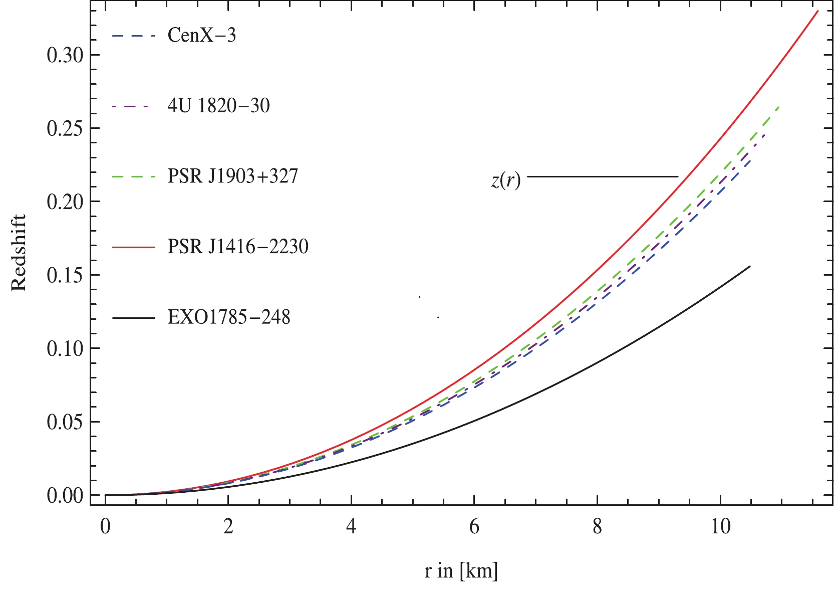
Figure 8. (color online) The red-shift function is plotted against radial coordinate, r for different experimental statistics of compact stars.
-
In this section, we study the stability of the anisotropic cosmic configuration. It is crucial for a stable anisotropic system that the propagation rate of sound waves traveling via an anisotropic fluid distribution should be less than that of electromagnetic radiation, i.e.,
$ 0<v_r^2<1 $ and$ 0<v_\perp^2<1 $ , where$ v_r $ and$ v_\perp $ are the components of sound speed expressed, respectively, as$ v_r^2 = \frac{{\rm d}p_r}{{\rm d}\rho},\quad v_\perp^2 = \frac{{\rm d}p_\perp}{{\rm d}\rho}. $

(61) This criterion is known as the causality condition [51] and is employed to examine the stability of the stellar system. The stability of a stellar model may also be examined via Herrera's cracking concept [52]. Cracking is produced when inward-directed radial forces of a perturbed stellar model alter the direction for a certain value of radial coordinates. Regarding this approach, the spherical cosmic body is potentially stable if it adheres to Herrera's cracking criterion indicated as
$ 0<|v_\perp^2-v_r^2|<1 $ . One of the intriguing characteristics of this scheme is that cracking is carefully linked to changes in local anisotropy. Figs. 9, 10, and 11 show that anisotropic distribution is in good concurrence with the causality condition as well as the cracking concept in the background of MBD theory.
Figure 9. (color online) Variation of radial speed of sound for 4U 1820-30 plotted against radial coordinate, r by taking
$\Phi_c = 0.3,\; m_\phi = 0.3,\; {\cal{B}} = 75.007\;\rm MeV/fm^3$ with different values of$\omega_{\rm BD}$ .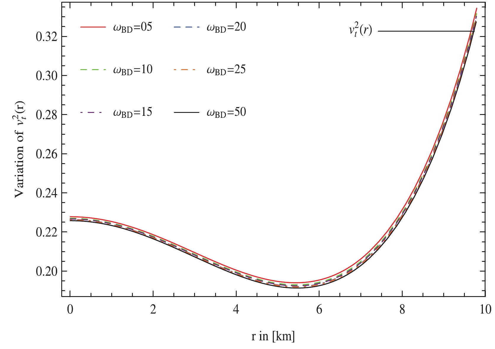
Figure 10. (color online) Variation of tangential speed of sound for 4U 1820-30 plotted against radial coordinate, r by taking
$\Phi_c = 0.3,\; m_\phi = 0.3,\; {\cal{B}} = 75.007\;\rm MeV/fm^3$ with different values of$\omega_{\rm BD}$ .
Figure 11. (color online) Variation of
$v_t^2 - v_r^2\;\& \;v_r^2 - v_t^2$ for 4U 1820-30 plotted against radial coordinate, r by taking$\Phi_c = 0.3,\; m_\phi = 0.3,\; {\cal{B}} = 75.007\;\rm MeV/fm^3$ with different values of$\omega_{\rm BD}$ .The adiabatic index is also another widely employed tool to check the stability of relativistic stellar systems. Chandrasekhar [53, 54, 55] investigated the dynamical stability of relativistic stellar structures versus infinitesimal radial adiabatic perturbation. Heintzmann and Hillebrandt [56] established that an anisotropic compact cosmic body will reach stability if the adiabatic index is greater than
$ \dfrac{4}{3} $ at each point within the stellar object. Moreover, if an increase in density generates an effective increase in pressure, the stellar system obeys a stiff EoS. A stellar geometry connected with a stiff EoS is harder to squeeze and more stable in contrast with a stellar configuration with a soft EoS. The EoS stiffness is evaluated through the adiabatic index given as$ \Gamma = \frac{p_r+\rho}{p_r}\frac{{\rm d}p_r}{{\rm d}\rho} = \frac{p_r+\rho}{p_r}v_r^2. $

(62) The value of this adiabatic index is more than
$ \frac{4}{3} $ for all considered values of the parameters$ m_\Phi,\; {\cal{B}} $ and$\omega_{\rm BD}$ which is in good accordance with the restraint [56]. Hence, the stellar configuration is potentially stable for the chosen values of MBD parameters.Finally, we verified the stability conditions for the prototype anisotropic celestial system employing three approaches: causality condition, Herrera's cracking approach, and adiabatic index. All these criteria imply the stability of the stellar model coupled to a massive scalar field.
-
Astrophysicists have investigated the dynamics of heavenly setups and their remainders to acquire insight into the cosmos mechanism. One of the hypothesized remainders are the QSs that arise from the collapse of NSs and are composed of up (u), down (d), and strange (s) quark flavors. The interaction amongst component quarks of these dense stellar configurations is described by the MIT bag model. These stellar configurations are highly dense compact stars whose constructions rely upon central and surface densities. In this study, we investigated the existence and stability of hypothetical objects, specifically, QSs in the context of MBD gravity. For this purpose, we constructed the field equations in the Jordan frame by choosing
${\cal{A}}(\Phi) = {\rm Exp}\Big[{\dfrac{\Phi^2}{(2 \omega_{\rm BD}+3)^{1/2}}}\Big]$ ,$ {\cal{L}}(\Phi) = \dfrac{1}{2}m_{\Phi}^2\Phi^2,\; m_\Phi = 0.3 $ , and$\omega_{\rm BD} = 05,\; 10,\; 15, \; 20,\; 25,\; $ $ 50$ . Additionally, we generated a solution to the field equations by supposing a well-behaved metric potential and embedding a class-one approach with the MIT bag model. The unknown constraints appearing in the anisotropic stellar model were determined by matching the inner spacetime to outer Schwarzschild spacetime. All the obtained results, viz., the behavior of matter variables as well as viability and stability of the resulting stellar model in the presence of a massive scalar field were explored and can be summarized as follows:● The evolution of the gravitational metric components of the spherically symmetric space-time, viz.,
$ {\rm e}^{\xi}\equiv g_{rr} $ and$ {\rm e}^{\eta}\equiv g_{tt} $ , with the fundamental conditions i.e.,$ {\rm e}^{\xi}\equiv g_{rr}|_{r = 0} = 1 $ and$ {\rm e}^{\eta}\equiv g_{tt}|_{r = 0}\ne0 $ , are presented in Fig. 1. It can be seen that both gravitational coefficients are positive, regular and monotonically increasing functions of the radial coordinate, r, which confirms that our stellar model is free from any physical and geometrical singularities.● The evolution of the matter variables viz., energy density, and components of stresses i.e.,
$ p_r $ ,$ p_t $ , against the radial coordinate r, can be observed in Figs. 2 and 3, respectively. We find that the energy density and stress components have maximum values at the core, decreasing progressively to attain the minimum values at the stellar surface as well as to confirm the physical acceptability of the obtained solutions. From Figs. 2 and 3, we emphasize again that our model is free from any physical or geometrical singularities for all selected parametric values of$ m_\Phi $ ,$\omega_{\rm BD}$ , and$ {\cal{B}} $ . Moreover, for the chosen values of the Bag constant viz.,$ {\cal{B}} $ , the existence of quark stellar configurations is ensured for$ {\cal{L}}(\Phi) = \dfrac{1}{2}m_{\Phi}^2\Phi^2 $ .● The behavior of the anisotropy viz.,
$ \Delta = p_t-p_r $ versus radial coordinate r, is shown in Fig. 4. It can be seen in this figure that both the stress components,$ p_r $ and$ p_t $ , are equal at the center i.e.,$ p_r(r = 0) = p_t(r = 0) $ , and afterwards, both the radial and transverse pressures differ from the center to the stellar surface, the transverse pressure stays positive, whereas the radial pressure vanishes at the boundary of the stellar configuration; this indicates that the pressure anisotropic function consistently stays positive all through the cosmic object. The graphical nature of pressure anisotropic function can be verified from the Fig. 4, which is positive with a concave upward growth pattern and is directed outwards.● The five kinds of energy conditions viz., NEC, WEC, SEC, DEC, and TEC, have been established which satisfied the considered values of the parameters as well as the bag constant. However, their graphic behavior can be observed from the Fig. 5, which also affirms that the interior of the stellar configuration consists of realistic or normal matter in our study.
● The growing behavior of the mass function and compactness factor versus the radial coordinate adheres to the Buchdahl criterion [49] for all considered values of MBD parameters. Moreover, the gravitational redshift of cosmic configuration increases with an increase in radial coordinate indicating more redshift in light for dense stellar structures compared with less dense celestial systems. The values of mass function, compactness factor, and gravitational redshift are in agreement with required physical conditions as can be observed in Figs. 6, 7, and 8.
● The stability analysis of a compact cosmic body study is also a crucial highlight. Concerning this, we examined the stability conditions for the prototype anisotropic stellar system via three approaches viz., causality condition, Herrera's cracking approach, and adiabatic index. All these criteria imply the stability of the cosmic model coupled to a massive scalar field. Sound speeds and Herrera's cracking concept are presented in Figs. 9, 10, and 11 against radial coordinates. Both the sound speeds are within the stable range of compact cosmic body i.e.,
$ 0<v_r^2<1 $ and$ 0<v_\perp^2<1 $ . Herrera's cracking concept [52]$ 0<|v_\perp^2-v_r^2|<1 $ is also justified to guarantee the potential stability of the stellar system. On the other hand, Fig. 12 exhibits the stability of the system of cosmic objects under adiabatic index$ \Gamma > \Gamma_c \equiv \dfrac{4}{3} $ in the background of MBD theory.
Figure 12. (color online) The adiabatic index for 4U 1820-30 plotted against radial coordinate, r by taking
$\Phi_c = 0.3,\; m_\phi = $ $ 0.3,\; {\cal{B}} = 75.007\;\rm MeV/fm^3$ with different values of$\omega_{\rm BD}$ .● We generated the physical properties of 4U 1820-30 due to different values of ω by tuning
$ m_{\Phi} $ to$ 0.3 $ and$ {\cal{B}} $ to$75.007\;\rm MeV/fm^3$ as shown in Table 1. In this Table, it is indicated that all physical quantities viz., the surface redshift$ Z_s $ , the mass ratio$ \dfrac{2M}{R} $ , the central pressure$ p_c $ , the surface density$ \rho_s $ , the central density$ \rho_c $ are always increasing when ω increases progressively. Furthermore in Table 2, we predicted several values of the physical parameters of the strange configurations observed i.e.,$ Z_s $ ,$ \dfrac{2M}{R} $ ,$ p_c $ ,$ \rho_s $ ,$ \rho_c $ , the radius R, for$ m_{\Phi} = 0.3 $ ,$ \omega = 15 $ and${\cal{B}} = 70\;\rm MeV/fm^3$ . In this regard, we affirm that the selected cosmic configurations are acceptable candidates for the ultra-dense hypothetical strange configurations by the results given in Tables 1 and 2. Similar to the values of high redshift, their surface densities are greater than the normal nuclear density as specified by Ruderman [62], Glendenning [63], and Herzog & Ropke [64]. Afterwards, in Table 3, we derived the values of the constants viz. A, B, C, and D, owing to several cosmic body candidates for the chosen values of the MBD parameters i.e.,$ m_{\Phi} = 0.3 $ ,$ \omega = 20 $ and${\cal{B}} = 75.007\;\rm MeV/fm^3$ shown in Table 3.It is worth mentioning that our results can be compared to phenomenological highlights inferred in other modified gravity theories like
$ f(R) $ . Since then,$ f(R) $ gravity theories were investigated by several researchers who pointed out the possibility that modified gravity can be used to resolve the problem of strange cosmic objects over a wide range of years. Specifically, Nashed and Capozziello [65, 66] have explored the notable solutions for anisotropic compact stellar configurations and charged spherically symmetric black holes in the background of the$ f(R) $ gravity and their stability analysis. Taking into account the$ f(R) $ gravity point of view for the secondary component of the GW190814 event, strange configurations possibilities are derived and also argued by Astashenok et al. in [67, 68]. In our study, we have chosen to work in the BD formalism, since the BD theory [15] is the prototypical alternative to GR and the most straightforward representative of scalar-tensor gravity [69-71]. Also in this formalism, the models are effectively viable with solar system tests, and the interior stellar configuration solution can match the exterior solution of the Schwarzshild. Compared with the outcomes given in [65-68], it is apparent that the$ f(R) $ theories are scalar-tensor theories in disguise with vanishing BD coupling$\omega_{\rm BD}$ and furnished with a complicated potential for the scalar degree of freedom$ f'(R) $ [69-71]. It is noteworthy that the obtained solutions are coherent with the GR partner and can be recovered for$ m_{\Phi} = 0 $ and$\omega_{\rm BD}\rightarrow \infty$ .Finally, it is worth mentioning that the solutions of the modified Einstein field equations for the compact configurations study in the presence of a massive scalar field under BD gravity are obtained by the embedding approach, thereby describing an anisotropic stellar model consisting of u, d, and s quark matter. Therefore, our anisotropic strange star model serves as a new path and interesting field for researchers to investigate ultra-dense compact stellar configurations.
Exploring physical features of anisotropic quark stars in Brans-Dicke theory with a massive scalar field via embedding approach
- Received Date: 2021-11-07
- Available Online: 2022-04-15
Abstract: The main aim of this study is to explore the existence and salient features of spherically symmetric relativistic quark stars in the background of massive Brans-Dicke gravity. The exact solutions to the modified Einstein field equations are derived for specific forms of coupling and scalar field functions using the equation of state relating to the strange quark matter that stimulates the phenomenological MIT-Bag model as a free Fermi gas of quarks. We use a well-behaved function along with the Karmarkar condition for class-one embedding as well as junction conditions to determine the unknown metric tensors. The radii of strange compact stars viz., PSR J1416-2230, PSR J1903+327, 4U 1820-30, CenX-3, and EXO1785-248, are predicted via their observed mass for different values of the massive Brans-Dicke parameters. We explore the influences of the mass of scalar field


 DownLoad: