


 Abstract
 HTML
HTML Reference
 Related
 PDF
PDF


-
One of the main goals of current relativistic heavy-ion collision experiments is to make clear the phase diagram of quantum chromo-dynamics (QCD) [1]. At vanishing baryon chemical potential, the transition from hadronic matter to quark–gluon plasma has been proved to be a crossover by lattice QCD [2]. Due to the fermion sign problem, lattice QCD can not calculate the cases at large baryon chemical potential. Some effective theories predict that the QCD system undergoes a first-order phase transition at high baryon density and low temperature [3–8]. From first-order phase transition to crossover, there is a critical point, which is a unique feature of the QCD phase diagram. Large fluctuations and correlations of conserved charges are expected at this critical point.
The high-order cumulants of conserved charges, reflecting their fluctuations, have been suggested for use in the search for the critical point [9–12]. Results from effective theories of QCD suggest that the non-monotonic behavior of the high-order cumulants is related to the critical point [13–15]. Particularly, sign change of the fourth-order net-proton cumulant has been used to search for the critical point in experiments [16, 17], while in Refs. [18, 19], the authors argued that the sign change is not sufficient to prove the presence of the critical point. Other work pointed out that the peak structure remains a solid feature and can be used as a clean signature of the critical point [20, 21].
Recently, the factorial cumulants, which are also known as the integrated multi-particle correlations, have received a lot of attention [22–30]. Multi-proton correlations have been found in the STAR data, at least at the lower energies [26, 29, 31]. It has been shown that the signs of the second- to fourth-order factorial cumulants are a useful tool to exclude regions in the QCD phase diagram close to the critical point using parametric representation of the Ising model [26]. The causes of sign change of factorial cumulants far away from the critical point compared with the cumulants have been analyzed in our recent work [32]. In the vicinity of the critical point, the sign and temperature dependence of factorial cumulants is almost the same as that of the cumulants. It has also been argued in Ref. [24] that the cumulants and factorial cumulants can not be distinguished in the vicinity of the critical point in a model of critical fluctuations.
Aside from non-monotonic behavior or sign changes of the cumulants and factorial cumulants, other behavior of the high-order cumulants has also been suggested for use in searching for the critical point, such as finite-size scaling [33, 34]. Finite-size scaling implies a fixed point. Usually, the fixed point is obtained from the scale transformation of the re-normalization group, resulting in the independence of rescaled thermodynamics on the system sizes at the critical point [35–37]. This feature has also been used to search for the critical point [38–40].
The QCD critical point, if it exists, is expected to belong to the same universality class as the three-dimensional Ising model [41–44]. Critical behavior of the corresponding thermodynamics in different systems that belong to the same universality class is the same as that which is supervised by the same critical exponents. Recently, many studies have been carried out to map the results of the three-dimensional Ising model to that of QCD [21, 45]. Usually, a linear ansatz is suggested between the QCD variables, temperature and net-baryon chemical potential, and the Ising variables, temperature and external magnetic field [46–49]. Cumulants of net-baryon number, which are the derivatives of the QCD free energy density with respect to net-baryon chemical potential, can be regarded as the combination of the derivatives with respect to temperature and magnetic field in the three-dimensional Ising model in the vicinity of the critical point. Since the critical exponent of external magnetic field is larger than that of temperature [50], the critical behavior of net-baryon number fluctuations is expected to be mainly controlled by the derivatives with respect to the external magnetic field, i.e., the fluctuations of the order parameter in the three-dimensional Ising model.
In this paper, using parametric representation and Monte Carlo simulations of the three-dimensional Ising model, we study and discuss the other kind of fixed point behavior in the temperature dependence of the normalized cumulants and factorial cumulants. Assuming the system formed in the heavy-ion collision experiments is in equilibrium, with a mapping from the Ising model to QCD, the fixed point behavior is also studied and discussed in the energy dependence of the normalized cumulants and factorial cumulants along different freeze-out curves, which may be helpful to locate the QCD critical point.
The paper is organized as follows. In section II, the three-dimensional Ising model and its parametric representation are introduced; parametric expressions of second- to fourth-order cumulants and factorial cumulants of the order parameter are derived; and, at the critical temperature, the independence on the external magnetic fields of the normalized cumulants are deduced. In section III, the temperature dependence of second- to fourth-order cumulants and factorial cumulants at different distances from the phase boundary and the fixed point behavior of the corresponding normalized cumulants are studied and discussed in the parametric representation. In section IV, the fixed point behavior of normalized second- to fourth-order cumulants and factorial cumulants is discussed in finite-size systems simulated by the Monte Carlo method. In section V, a mapping from the Ising model to QCD is introduced; and the fixed point behavior of the energy dependence of the normalized (factorial) cumulants is studied and discussed. Finally, conclusions and summary are given in section VI.
-
The three-dimensional Ising model is defined as follows,
$ \mathcal{H} = -J\sum\limits_{\langle i,j\rangle}{s}_{i}{s}_{j}-H\sum\limits_{i}{s}_{i}, $

(1) where
$ \mathcal{H} $ is the Hamiltonian,$ s_{i} $ is spin at site i on a simple cubic lattice which can take only two values$ \pm 1 $ . J is the interaction energy between nearest-neighbor spins$ \langle i,j\rangle $ . H represents the external magnetic field. The magnetization M (the order parameter) is$ M = \frac{1}{V}{\langle \sum\limits_{i}{s_{i}}\rangle} = \frac{\langle s \rangle}{V}, $

(2) $ s = \sum_{i}{s_{i}} $ and$ V = L^d $ denotes the total spin and volume of the lattice, respectively, where$ d = 3 $ is the dimension of the lattice and L is the number of lattice points of each direction on the cubic lattice. The magnetization is dependent on the external magnetic field H and the reduced temperature$ t = (T-T_{\rm c})/{T_{\rm c}} $ , where$ T_{\rm c} $ is the critical temperature. At$ t>0 $ is the crossover side.$ t<0 $ is the first-order phase transition side.High-order cumulants of the order parameter can be obtained from the derivatives of magnetization with respect to H at fixed t,
$ \left.\kappa_{n}(t,H) = \left(\frac{\partial^{n-1} M}{\partial H^{n-1}}\right)\right|_{t}. $

(3) In particular, the second- to fourth-order cumulants are as follows,
$ \begin{aligned}[b] \kappa_2 =& \frac{1}{V}{\langle (\delta s)^2 \rangle}, \\ \kappa_3 =& \frac{1}{V}{\langle (\delta s)^3 \rangle}, \\ \kappa_4 =& \frac{1}{V}(\langle (\delta s)^4 \rangle-3\langle(\delta s)^2 \rangle^2), \end{aligned} $

(4) where
$ \delta s = s-\langle s\rangle $ .Turning to the parametric representation of the three-dimensional Ising model, magnetization M and reduced temperature t can be parameterized by two variables R and
$ \theta $ [51, 52],$ M = m_0R^{\beta}\theta,\; \; \; \; \; \; t = R(1-\theta^2). $

(5) The equation of state of the Ising model can be given by the parametric representation in terms of R and
$ \theta $ as$ H = h_0R^{\beta\delta}h(\theta). $

(6) Where
$ m_0 $ in Eq. (5) and$ h_0 $ in Eq. (6) are normalization constants. These are fixed by imposing the normalization conditions$ M(t = -1,H = +0) = 1 $ and$ M(t = 0, $ $ H = 1) = 1 $ .$ \beta $ and$ \delta $ are critical exponents of the three-dimensional Ising universality class with values 0.3267(10) and 4.786(14), respectively [53].If M, t and h are analytic functions of
$ \theta $ , the analytic properties of the equation of state are satisfied [54]. The analytic expression of the high-order cumulants can be derived in the parametric representation. What is more, the function$ h(\theta) $ is an odd function of$ \theta $ because the magnetization is an odd function of the external magnetic field$ M(-H) = -M(H) $ .One simple function of
$ h(\theta) $ obeying all the requirements is as follows,$ h(\theta) = \theta(3-2\theta^{2}). $

(7) This is a mean-field approximation of representation for the equation of state of the three-dimensional Ising model to order
$ \varepsilon^{2} $ , where$ \varepsilon $ is a parameter related to the number of dimensions of space.$ \varepsilon $ -expansion is one of the techniques to explore critical phenomena. This is enough for our purpose, although the parametric representation is also known up to order$ \varepsilon^{3} $ [52]. There is an excellent agreement between the scaling magnetization data from Monte Carlo simulation and the equation of state in the parametric representation [55].When taking the approximate values of the critical exponents
$ \beta = 1/3 $ and$ \delta = 5 $ (accurate enough for our purpose), the first four order cumulants in the parametric representation are as follows:$ \begin{aligned}[b]\kappa_{1}(t,H) =& m_0R^{1/3}\theta,\\ \kappa_{2}(t,H) =& \frac{m_0}{h_0}\frac{1}{R^{4/3}(2\theta^2+3)},\\ \kappa_{3}(t,H) =& \frac{m_0}{h_0^2}\frac{4\theta(\theta^2+9)}{R^{3}(\theta^2-3)(2\theta^2+3)^3},\\ \kappa_{4}(t,H) =& 12\frac{m_0}{h_0^3}\frac{(2\theta^8-5\theta^6+105\theta^4-783\theta^2+81)}{R^{14/3}(\theta^2-3)^3(2\theta^2+3)^5}.\end{aligned} $

(8) The reduced temperature t and external magnetic field H are functions of R and
$ \theta $ provided by Eq. (5) and Eq. (6). At fixed H, R can be represented in terms of$ \theta $ by Eq. (6). As a consequence, cumulants in Eq. (8) just depend on$ \theta $ , as does the reduced temperature t in Eq. (5). There are three kinds of special values of$ \theta $ , which are$ \theta = \theta_{n}^{\rm max} $ for the peak of$ \kappa_n $ if the peak exists,$ \theta = \theta_{n}^{\rm min} $ for the valley of$ \kappa_n $ if the valley exists,$ \theta = 1 $ for the reduced temperature$ t = 0 $ (the critical temperature) at a positive magnetic field (or$ \theta = -1 $ for$ t = 0 $ at a negative magnetic field).The first two cases imply the ratios (the factor of H is offset in the ratios) of the peak hight to the valley depth for
$ \kappa_4 $ ,$ \kappa_5 $ and$ \kappa_6 $ are universal and independent of H. They are approximately$ -28 $ ,$ -0.1 $ , and$ -6 $ , respectively, for$ H>0 $ [16, 32].At a positive magnetic field, temperature dependence of even-order cumulants shows a positive peak in the vicinity of the critical temperature, while it is a negative valley for the odd-order cumulants [32]. Normalizing the even-order cumulants by their peak hight
$ \kappa_{2n}^{\rm max}, n = $ $ 1,2,3... $ , and the odd-order cumulants by the absolute value of the valley depth$ \vert\kappa_{2n+1}^{\rm min}\vert, n = 1,2,3... $ , then from the last case, one can get a fixed point behavior of temperature dependence of normalized cumulants$ \kappa_n^{\rm Norm} $ for different values of H at$ t = 0 $ .Especially, one can get the second- to fourth-order normalized cumulants,
$ \begin{aligned}[b]\kappa_{2}^{\rm Norm} =& \kappa_{2}/\kappa_{2}^{\rm max},\\ \kappa_{3}^{\rm Norm} =& \kappa_{3}/\vert\kappa_{3}^{\rm min}\vert, \\ \kappa_{4}^{\rm Norm} =& \kappa_{4}/\kappa_{4}^{\rm max}.\end{aligned}$

(9) At any positive magnetic field, values of second- to fourth-order normalized cumulants at
$ t = 0 $ are as follows,$ \begin{aligned}[b]\kappa_{2}^{\rm Norm}(t = 0) =& \frac{\kappa_{2}(\theta = 1)}{\kappa_{2}(\theta = \theta_2^{\rm max})}\approx 0.58, \\ \kappa_{3}^{\rm Norm}(t = 0) =& \frac{\kappa_{3}(\theta = 1)}{\vert \kappa_{3}(\theta = \theta_3^{\rm min})\vert}\approx -0.51,\\ \kappa_{4}^{\rm Norm}(t = 0) = &\frac{\kappa_{4}(\theta = 1)}{\kappa_{4}(\theta = \theta_4^{\rm max})}\approx 0.49. \end{aligned} $

(10) In fact, cumulants can be normalized by their values at any
$ \theta $ to get the fixed point behavior at the critical temperature, but among those the most convenient choice would be normalization by the extreme values which can be identified easily from measured data.The second- to fourth-order factorial cumulants can be expressed by the cumulants as follows [28],
$ \begin{aligned}[b] C_{2} =& \kappa_{2}-\kappa_{1},\\ C_{3} =& \kappa_{3}-3\kappa_{2}+2\kappa_{1},\\ C_{4} =& \kappa_{4}-6\kappa_{3}+11\kappa_{2}-6\kappa_{1}.\end{aligned}$

(11) They can also be normalized by their maximum or the absolute values of their minimum as follows,
$ \begin{aligned}[b] C_{2}^{\rm Norm} =& C_{2}/C_{2}^{\rm max},\\ C_{3}^{\rm Norm} =& C_{3}/\vert C_{3}^{\rm min}\vert, \\ C_{4}^{\rm Norm} =& C_{4}/C_{4}^{\rm max}.\end{aligned} $

(12) Because the factorial cumulants mix different orders of cumulants as shown in Eq. (11), far away from the critical point the behavior of factorial cumulants is very different from the same-order cumulants [32]. It also appears that there may be no fixed point behavior in the temperature dependence of the factorial cumulants at the critical temperature for different external magnetic fields. But one should keep in mind that, in the vicinity of the critical point, cumulants and the same-order factorial cumulants can not be distinguished. The higher the order of the factorial cumulant, the more dominant the role of the same-order cumulant in its critical behavior.
-
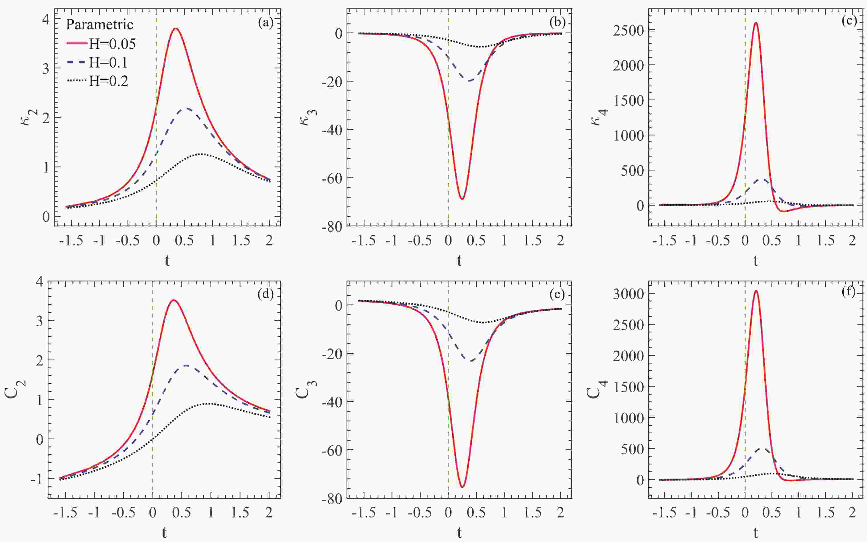
As the value of H increases, it moves far away from the phase boundary. At three different magnetic field values
$ H = 0.05, 0.1, 0.2 $ , the temperature dependence of second- to fourth-order cumulants and factorial cumulants are studied in the parametric representation of the three-dimensional Ising model, as shown in Fig. 1(a)–(f). The vertical green dashed line shows the critical temperature.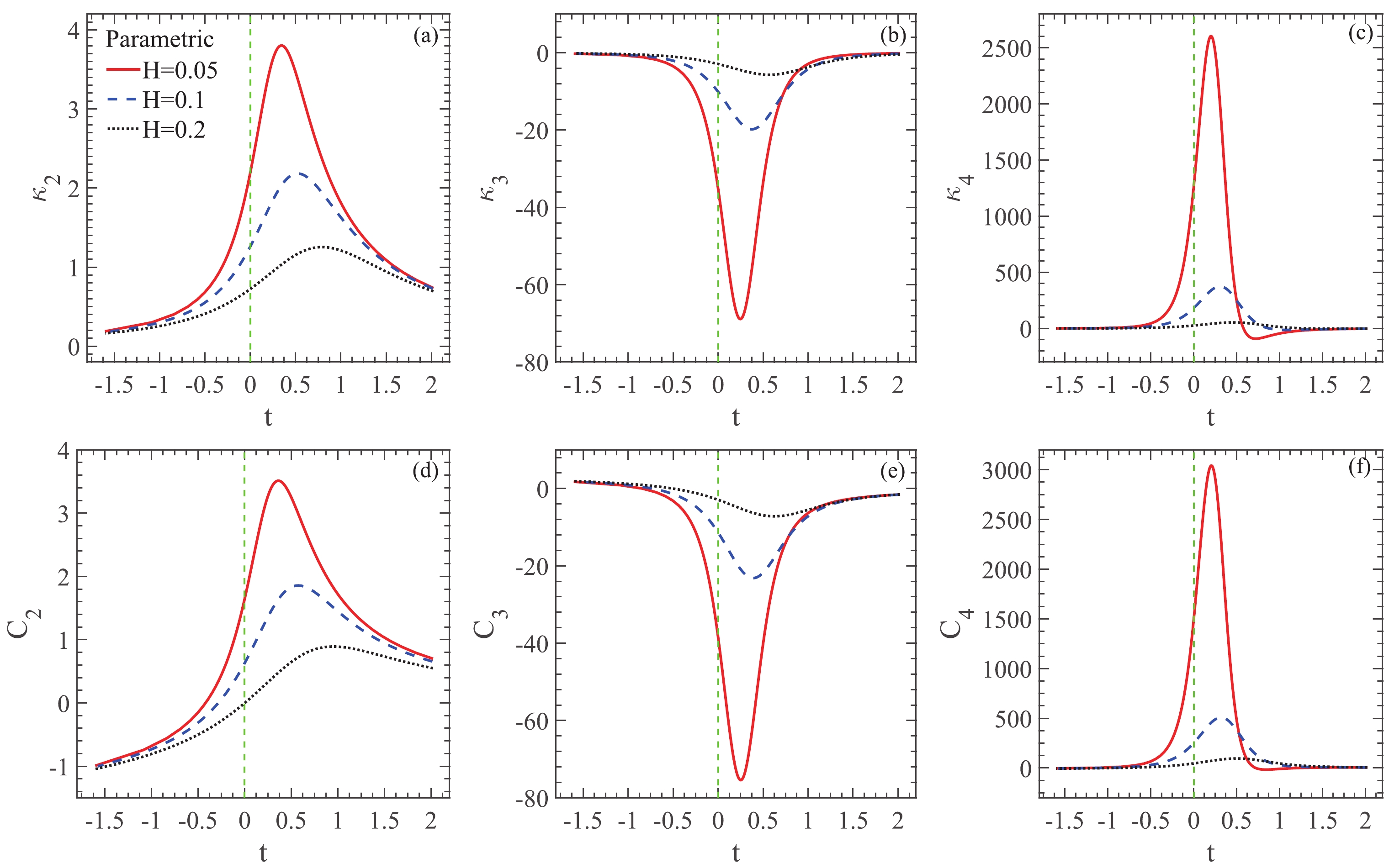
Figure 1. (color online) Temperature dependence of
$ \kappa_2 $ (a),$ \kappa_3 $ (b),$ \kappa_4 $ (c),$ C_2 $ (d),$ C_3 $ (e) and$ C_4 $ (f) at three different values of external magnetic fields,$ H = 0.05 $ ,$ 0.1 $ and$ 0.2 $ , in the parametric representation of the three-dimensional Ising model. The green dashed line shows the critical temperature.It is clear that, as the value of H decreases, the qualitative temperature dependence of
$ \kappa_2 $ does not change, all showing a peak structure in the vicinity of the critical temperature. But the peak becomes higher, sharper and closer to the critical temperature, as shown in Fig. 1(a). The similar situation occurs for$ \kappa_3 $ in Fig. 1(b) and$ \kappa_4 $ in Fig. 1(c). The smaller the value of H, the closer to the phase boundary, the more singular the behavior of cumulants.In the vicinity of the critical temperature, trends of temperature dependence of factorial cumulants are similar to the same-order cumulants, as shown in Fig. 1(d)–(f). When far from the critical temperature, the sign of factorial cumulants can possibly change, which is consistent with the results in Ref. [32].
The normalized cumulants and factorial cumulants are shown in Fig. 2. The vertical green dashed line shows the critical temperature, while the horizontal green dashed line shows the value of normalized cumulants at the critical temperature, which are inferred from Eq. (10).
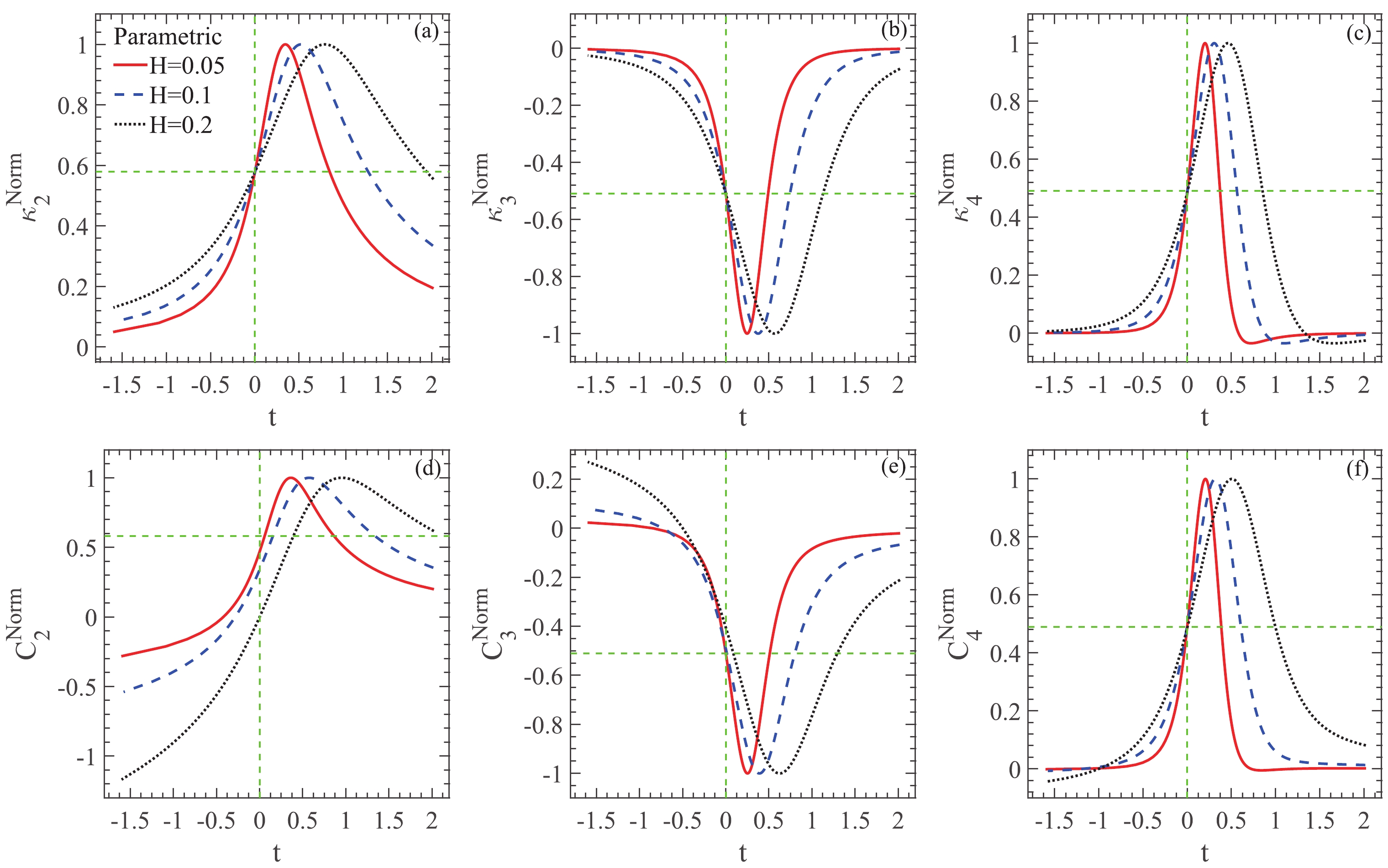
Figure 2. (color online) Temperature dependence of
$ \kappa_2^{\rm Norm} $ (a),$ \kappa_3^{\rm Norm} $ (b),$ \kappa_4^{\rm Norm} $ (c),$ C_2^{\rm Norm} $ (d),$ C_3^{\rm Norm} $ (e) and$ C_4^{\rm Norm} $ (f) at three different values of external magnetic fields,$ H = 0.05 $ ,$ 0.1 $ and$ 0.2 $ , in the parametric representation of the three-dimensional Ising model. The crossing point of the green dashed lines is the fixed point.It is clear that for
$ \kappa_2^{\rm Norm} $ ,$ \kappa_3^{\rm Norm} $ and$ \kappa_4^{\rm Norm} $ shown in Fig. 2(a)–(c), a common feature occurs. That is the fixed point behavior at the critical temperature. At different values of H, values of$ \kappa_2^{\rm Norm} $ are the same at the critical temperature. This is independent of the distance to the phase boundary. So are the values of$ \kappa_3^{\rm Norm} $ and$ \kappa_4^{\rm Norm} $ . The fixed point is exactly at the crossing point of the two dashed green lines. That is to say, the values of the normalized cumulants at t are consistent with Eq. (10).As shown in Fig. 2(c), the valley depths for
$ \kappa_4^{\rm Norm} $ at$ H = 0.05, 0.1, 0.2 $ are almost the same [16]. One can conclude that the ratios of the peak hight to the valley depth are independent of H. For the fourth-order cumulant, in some cases, if the peak can not be determined, one can normalize it by its valley depth. The fixed point behavior also exists.All in all, the ratios of the value of even-order cumulants (odd-order cumulants) at critical temperature to its peak value (valley depth) is independent of the external magnetic fields. This results in a fixed point behavior in the temperature dependence of normalized cumulants, which may be helpful in the search for the critical temperature.
Turning to the normalized factorial cumulants shown in Fig. 2(d)–(f), it is clear that far from the critical temperature, each order of factorial cumulant has sign changes with increasing H. That is to say, far from the phase boundary, there exists a sign difference between cumulants and the same-order factorial cumulants.
Let us pay attention to the fixed point behavior of the normalized factorial cumulants. There is no fixed point behavior in the temperature dependence of
$ C_2^{\rm Norm} $ , as shown in Fig. 2(d), which is in line with the inference from the relation between factorial cumulants and cumulants in Eq. (11).For
$ C_3^{\rm Norm} $ in Fig. 2(e), the fixed point behavior is not so clear. But the fixed point occurs again in$ C_4^{\rm Norm} $ , as shown in Fig. 2(f). The position of the fixed point is just at the crossing point of the two green dashed lines, consistent with$ \kappa_4^{\rm Norm} $ . In fact, the higher the order of the cumulants, the more sensitive the cumulants are to the correlation length, the more dominant the role of the cumulants in the critical behavior of the same-order factorial cumulants. So fixed point behavior occurring in$ C_4^{\rm Norm} $ again is not hard to understand. -
Using the Monte Carlo simulation method, the fixed point behavior is tested in finite-size systems at three different values of external magnetic fields. Because of the finite-size effects, the temperature dependence curves of the cumulants will shift to the higher temperature side until the system size is large enough to sufficiently converge to the thermodynamic limit. The typical size is determined by the saturation of size dependence of an observable at a given magnetic field [56]. For cumulants up to the fourth order at three different magnetic field values
$ H = 0.05 $ ,$ 0.07 $ , and$ 0.1 $ , lattice sizes$ L = 14 $ ,$ 12 $ and$ 10 $ respectively are sufficient to converge to the thermodynamic limit. For each value of H, the simulations are performed at$ 5 $ values of inverse temperature$ J/T = 0.202 $ ,$ 0.212 $ ,$ 0.222 $ ,$ 0.232 $ and$ 0.242 $ near the critical temperature$ T_c/J \approx 4.51 $ , where the value of interaction energy J is set to$ 1 $ . The Wolff cluster algorithm is used with helical boundary conditions [57]. At each pair of$ (H, J/T) $ ,$ 48 $ million independent configurations are generated and used in a Ferrenberg–Swendsen reweighting analysis to calculate observables at intermediate temperature values [58].Results of the second- to fourth- order normalized cumulants and factorial cumulants are shown in Fig. 3(a)–(f), respectively. It is clear that the fixed point behavior in temperature dependence of
$ \kappa_2^{\rm Norm} $ ,$ \kappa_3^{\rm Norm} $ and$ \kappa_4^{\rm Norm} $ still exists, as shown in Fig. 3(a)–(c). The crossing point of the two green dashed lines shows the position of the fixed point. The corresponding temperature is about one percent lower than the critical temperature. What is more, the higher the order of the cumulants, the closer the fixed point is to the critical temperature. In addition, the values of the normalized cumulants at fixed points are different from those in the parametric representation. This can be caused by the finite-size system, the choice of function$ h(\theta) $ and the different quantitative temperature dependence of$ \kappa_n $ in Monte Carlo simulation and the parametric representation.
Figure 3. (color online) Temperature dependence of
$ \kappa_2^{\rm Norm} $ (a),$ \kappa_3^{\rm Norm} $ (b) and$ \kappa_4^{\rm Norm} $ (c),$ C_2^{\rm Norm} $ (d),$ C_3^{\rm Norm} $ (e) and$ C_4^{\rm Norm} $ (f) at three different values of external magnetic field,$ H = 0.05 $ ,$ 0.07 $ and$ 0.1 $ , in the three-dimensional Ising model simulated by Monte Carlo method. The crossing point of the green dashed lines is the fixed point for the upper panel. The positions of the green dashed lines in the lower panel are kept consistent with those in the upper panel.Comparing the temperature dependence of normalized factorial cumulants shown in Fig. 3(d)– (f) with the same-order normalized cumulants shown in Fig. 3(a)–(c), there are no significant differences between them. That is because the temperatures are close to critical. This result is consistent with that in Refs. [24, 32], that these two kinds of cumulants can not be distinguished in the vicinity of the critical point. So it is not hard to understand that except for
$ C_2^{\rm Norm} $ , there is obvious fixed point behavior in the temperature dependence in$ C_3^{\rm Norm} $ and$ C_4^{\rm Norm} $ , as shown in Fig. 3(e) and (f). The positions of the green dashed lines are set the same as those in the same-order normalized cumulants. It is not hard to infer that the temperature of the fixed point in the normalized factorial cumulants is almost the same as that in the normalized cumulants.All in all, at different external magnetic field values in finite-size systems of the three-dimensional Ising model, the temperature dependence of the normalized cumulants or factorial cumulants (at least from the third-order) form a fixed point just about one percent distant from the critical temperature. Comparing the positions of the peak and the sign change, the fixed point of the normalized cumulants or factorial cumulants is much closer to the critical temperature.
-
In the current study we focus on the equilibrium properties of the cumulants and factorial cumulants. Thus the non-equilibrium effects are not taken into account [59].
In order to apply the results of this paper to the heavy-ion collision experiments to search for the QCD critical point, it is essential to specify the map between the Ising variables t, H to the QCD variables temperature T and baryon chemical potential
$ \mu_B $ . The t axis is tangential to the first-order phase transition line at the QCD critical point. The angle between the horizontal (fixed T) lines on the QCD phase diagram and t axis is$ \alpha $ . For simplicity, we assume that the H axis is perpendicular to the t axis after the map to the$ T-\mu_B $ plane, which has been studied in Ref. [48]. Then a linear mapping relations can be obtained as follows:$ \begin{aligned}[b] \frac{T-T_{\rm cep}}{\Delta T} =& -\cos\alpha\frac{H}{\Delta H}+\sin\alpha \frac{t}{\Delta t},\\ \frac{\mu_B-\mu_{Bc}}{\Delta \mu_B} =& -\sin\alpha\frac{H}{\Delta H}-\cos\alpha \frac{t}{\Delta t},\end{aligned} $

(13) where
$ T_{\rm cep} $ ,$ \mu_{Bc} $ represent the temperature and baryon chemical potential at the QCD critical point, and$ \Delta T $ and$ \Delta \mu_B $ denote the width of the critical regime in the QCD phase diagram. Because the location of the critical point and the width of the critical regime for QCD are not known, the suggestion that$ \Delta \mu_B \approx 0.1 $ GeV from model calculations [60] and lattice QCD calculations [61] is used. We set$ \Delta \mu_B = 0.1 $ GeV and$ \mu_{Bc} = 0.25 $ GeV as in Ref. [59].$ \Delta H $ and$ \Delta t $ denote the width of the critical regime in the Ising variables. For simplicity, we set$ \Delta H = 0.4 $ and$ \Delta t = 2 $ . The fixed point behavior is not sensitive to the width of the critical regime in the Ising variables. For more information to define the critical regime, see Ref. [59].Finally, the freeze-out curve is assumed to be below the crossover/first-order phase transition line. An empirical parametrization of the heavy-ion collision data from Ref. [62] can be used to describe the freeze-out curves,
$ T_f(\mu_B) = a-b{\mu_B}^2-c{\mu_B}^4,$

(14) where
$ a = 0.166 $ GeV,$ b = 0.139 $ GeV$ ^{-1} $ , and$ c = 0.053 $ GeV$ ^{-3} $ . At a range of small$ \mu_B $ (0.15 <$ \mu_B $ < 0.35 GeV),$ T_f $ is varying approximately linearly with$ \mu_B $ in this study. The angle between the straight line of$ T_f(\mu_B) $ and the horizontal (fixed T) line on the QCD$ T-\mu_B $ plane is very small. For simplicity, we assume the freeze-out curve is approximately parallel to the t direction which has been mapped to the QCD phase diagram.A straightforward phase diagram of the three-dimensional Ising model on the
$ t-H $ plane and one possible sketch of the$ t-H $ axes mapped onto the$ T-\mu_B $ plane of QCD are shown in Fig. 4(a) and (b), respectively. Thus three lines parallel to the t axis from left to right at three different values of H in Fig. 4(a) can be simply mapped to three freeze-out curves from top to bottom in QCD as shown in Fig. 4(b).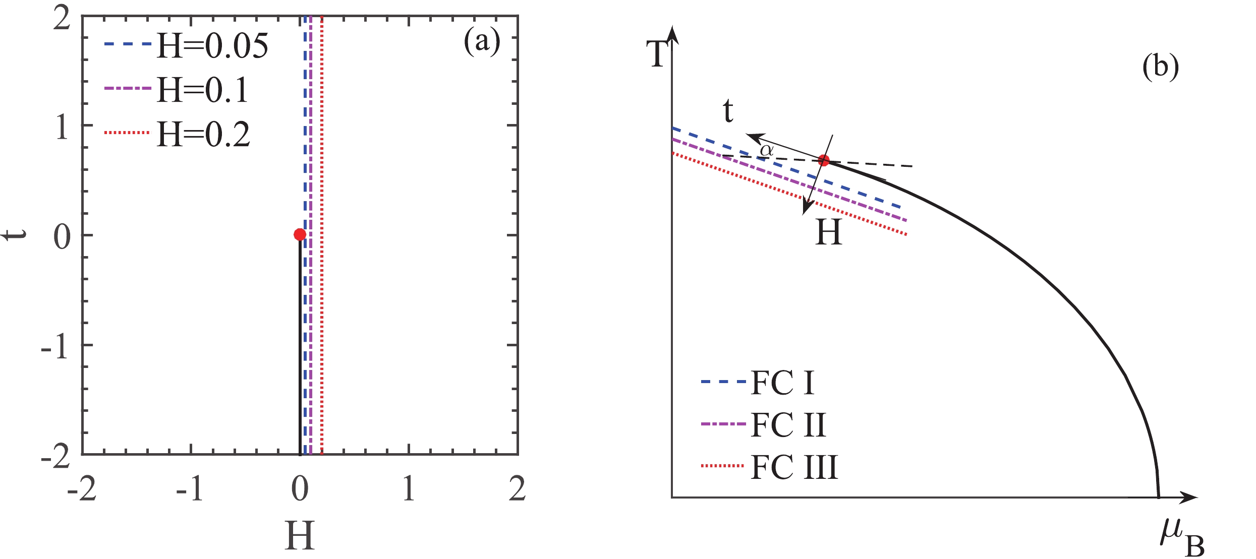
Figure 4. (color online) Phase diagram on
$ t-H $ plane of the three-dimensional Ising model (a). Sketch of the$ t-H $ axes mapped onto the QCD$ T-\mu_B $ plane (b). The black solid line and the red point are the first-order phase transition line and the critical point, respectively. The t axis is tangential to the QCD phase boundary at the critical point. The H direction is set to be perpendicular to the t axis. The three lines parallel to the phase boundary from left to right (H = 0.05, 0.1 and H = 0.2) of Ising model (a) are mapped to the three freeze-out curves which are parallel to the t axis from top to bottom (FC I, FC II and FC III) in QCD$ T-\mu_B $ plane (b).Based on this mapping and using Eq. (13), the temperature dependence of normalized cumulants and factorial cumulants at the three different values for H can be converted to the
$ \mu_B $ dependence of normalized cumulants and factorial cumulants along the three different freeze-out curves.Turning to the heavy-ion collision experiments, using the energy (
$ \sqrt s $ ) dependence of$ \mu_B $ given in Ref. [62],$ \mu_B(\sqrt s) = \frac{d_0}{d_1\sqrt s +1}, $

(15) where
$ d_0 = 1.308 $ GeV,$ d_1 = 0.273 $ GeV$ ^{-1} $ , one can get the energy dependence of normalized cumulants and factorial cumulants along the three different freeze-out curves.Supposing the angle
$ \alpha = 3^{\circ} $ , based on the parametric representation of the Ising model, energy dependence of the second- to fourth-order normalized cumulants and factorial cumulants along the three freeze-out curves are shown in Fig. 5(a)–(f), respectively. The vertical green dashed lines show the critical energy$ {\sqrt s}_c = 15.5 $ GeV which corresponds to$ \mu_{Bc} = 0.25 $ GeV at the QCD critical point through Eq. (15). It is clear that the fixed point behavior exists at$ {\sqrt s}_c $ in the energy dependence of$ \kappa_2^{\rm Norm} $ to$ \kappa_4^{\rm Norm} $ , as shown in Fig. 5(a)–(c), respectively. The values of the normalized cumulants at the fixed point shown by the horizontal green dashed line are slightly changed compared to the values given by Eq. (10) because of the mapping from the Ising variables to the QCD variables.
Figure 5. (color online) Energy dependence of
$ \kappa_2^{\rm Norm} $ (a),$ \kappa_3^{\rm Norm} $ (b) and$ \kappa_4^{\rm Norm} $ (c),$ C_2^{\rm Norm} $ (d),$ C_3^{\rm Norm} $ (e) and$ C_4^{\rm Norm} $ (f) along three different freeze-out curves as shown in Fig. 4(b). The vertical green dashed lines show the energy$ {\sqrt s}_c $ corresponding to$ \mu_{Bc} $ . The horizontal green dashed lines show the value of the normalized cumulants at the fixed point for the upper panel. The positions of the green dashed lines in the lower panel are kept consistent with those in the upper panel.For the normalized factorial cumulants shown in Fig. 5(d)–(f), the fixed point behavior occurs from the fourth-order one, and its position is consistent with that in
$ \kappa_4^{\rm Norm} $ .The fixed point behavior in the energy dependence of the normalized cumulants is derived directly from the linear mapping in Eq. (13), where
$ \Delta H $ ,$ \Delta t $ and the angle$ \alpha $ are all set to fixed values in this paper. The influence of these three parameters on the fixed point behavior should be explained. The fixed point behavior still exists with the variation of these three parameters. Different values of$ \Delta H $ and$ \Delta t $ leave the energy at the fixed point almost unchanged. They just influence the range of the energy (the range of$ \mu_B $ ) after the mapping. Small values of$ \alpha $ (like$ 3^{\circ} $ used in this paper) have little influence on the fixed point behavior, while high values of$ \alpha $ not only change the range of the energy, but also shift the fixed point away from$ {\sqrt s}_c $ (but one should notice that a small value for$ \alpha $ should be closer to the truth here).One other problem that should be discussed is how one can get different freeze-out curves in the heavy-ion collisions. In fact, the centrality dependence of the chemical freeze-out temperature and baryon chemical potential have been studied in Refs. [63, 64]. Although the chemical freeze-out temperature does not vary much with centralities, the temperature interval between the three different freeze-out curves can be very small. If we set
$ T_{\rm cep} = 0.18 $ GeV and$ \Delta T = T_{\rm cep}/8 $ , which has been used in Ref. [59], the critical regime of QCD temperature is$ \Delta T $ = 0.0225 GeV. When the external magnetic field H changes from 0.05 to 0.2 at the same t, after mapping to the QCD variables through Eq. (13), the freeze-out temperature interval is just about$ 0.0084 $ GeV. What is more, baryon chemical potential increases from peripheral to the most central collisions [64]. It is enough for one to get different freeze-out curves at different centralities. So the centrality controlling the freeze-out curves in the QCD phase diagram may play a similar role of the external magnetic field H of the Ising model.Under the mapping from the three-dimensional Ising model to QCD, the fixed point behavior may be expected in the energy dependence of normalized net-proton (factorial) cumulants in heavy-ion collision experiments. This feature can be used to locate the QCD critical point.
-
By using the parametric representation of the three-dimensional Ising model, the temperature dependence of the second- to fourth-order cumulants and factorial cumulants of the order parameter has been studied. The qualitative behavior of temperature dependence of cumulants does not change with the varying external magnetic field in the vicinity of the critical temperature. Nor does that of the factorial cumulants.
The fixed point behavior in the temperature dependence of normalized cumulants at the critical temperature for different magnetic fields has been deduced and shown.
By Monte Carlo simulation of the three-dimensional Ising model, the fixed point behavior in the temperature dependence of normalized second- to fourth-order cumulants has been checked in finite-size systems. The fixed point behavior still exists just about one percent distant from the critical temperature, which is much closer to the critical temperature than the peak structure or sign change shown in the temperature dependence of the cumulants.
For the normalized factorial cumulants, the fixed point behavior also survives from at least the fourth-order cumulants, both in the parametric representation and finite-size systems, which reflects the fact that the critical behavior of factorial cumulants is dominated by the corresponding cumulants. The higher the order of the factorial cumulant, the more dominant the role of the same-order cumulant in its critical behavior.
Through a mapping from the three-dimensional Ising model to QCD, the fixed point behavior is also found in the energy dependence of the normalized cumulants (or fourth-order factorial cumulants) along different freeze-out curves. The fixed point is very close to the critical energy (corresponding to the baryon-chemical potential at the QCD critical point). It is promising that this method is applicable to locate the QCD critical point in heavy-ion collision experiments.
More generally it must be emphasized that all of the results here rely on the equilibrium of the system. Whether the fixed point behavior survives in the non-equilibrium cumulants needs further study. What is more, further studies of different ways of mapping from the Ising model to QCD would be helpful.
Fixed point behavior of cumulants in the three-dimensional Ising universality class
- Received Date: 2021-08-02
- Available Online: 2022-02-15
Abstract: High-order cumulants and factorial cumulants of conserved charges are suggested for the study of the critical dynamics in heavy-ion collision experiments. In this paper, using the parametric representation of the three-dimensional Ising model which is believed to belong to the same universality class as quantum chromo-dynamics, the temperature dependence of the second- to fourth-order (factorial) cumulants of the order parameter is studied. It is found that the values of the normalized cumulants are independent of the external magnetic field at the critical temperature, which results in a fixed point in the temperature dependence of the normalized cumulants. In finite-size systems simulated using the Monte Carlo method, this fixed point behavior still exists at temperatures near the critical. This fixed point behavior has also appeared in the temperature dependence of normalized factorial cumulants from at least the fourth order. With a mapping from the Ising model to QCD, the fixed point behavior is also found in the energy dependence of the normalized cumulants (or fourth-order factorial cumulants) along different freeze-out curves.


 DownLoad: