


 Abstract
 HTML
HTML Reference
 Related
 PDF
PDF


-
It is known that the history of the study of dibaryons, such as H and
$ {d^*} $ particles, can be traced back to about 60 years ago (refer to the review articles by Clement [1, 2]). Theoretically, the possible dibaryon states have been carefully investigated with many approaches from the hadronic degrees of freedom (HDF) to the quark degrees of freedom (QDF). In 2009, the evidence of$ {d^*} $ was firstly reported by CELSIUS/WASA and WASA@COSY Collaborations [3-6]. Observations of the existence of such a dibaryon were claimed in their series of experiments. This is because that their observed peak cannot simply be understood by the role from either the intermediate Roper excitation or from the t-channel intermediate$ \Delta\Delta $ state, except by introducing a new intermediate resonance with its mass, width, and quantum numbers being$ 2370\sim $ $ 2380\; \rm{MeV} $ ,$ 70\sim 80\; \rm{MeV} $ , and$ I(J^P) = 0(3^+) $ , respectively. Since the baryon number of this resonance is 2, one believes it may just be the light-quark-only dibaryon$ {d^*}(2380) $ that has been hunted for several decades.According to the mass of
$ {d^*} $ and the relevant thresholds of the two-baryon ($ {\Delta \Delta} $ ), two-baryon plus one-meson ($ NN\pi $ ), and two-baryon plus two-meson ($ NN\pi\pi $ ) channels nearby, one could believe the threshold (or cusp) effect should be much smaller in the case of this resonance than that in the cases of the exotic XYZ resonances [7-10]. And due to its narrow width, one may think of this dibaryon as a state with, at least, a hexaquark-dominated structure. Up to now, several theoretical proposals for its internal structure have been investigated. Among them, two proposed structures have attracted much attention. The first one comes from the study in QDF. The calculation showed that$ {d^*} $ has a compact structure and is a candidate of an exotic hexaquark-dominated resonant state [11-17]. (A similar assumption regards the$ d^* $ state being a deeply bound state of two Δs [18, 19], however its width is larger than the measured value.) The other calculation, in HDF, considers it as a molecular-like hadronic state, which originates from an assumption of a three-body resonance$ \Delta N\pi $ or a molecular-like state$ D_{12}\pi $ [20-23]. Although the mass and the partial widths of the double pionic decays of such a hypothetical dibaryon resonance can be reasonably reproduced by both proposed structures, the interpretations in the two proposals are entirely different. Of course, there are many other studies for understanding the structure of$ {d^*} $ and$ pp\to \pi^+d $ reaction, for instance, the triple di-quark model [24] and the triangle singularity mechanism [25]. Whether they can systematically explain all existing experimental data still needs to be further tested. Therefore, it is necessary to look for other physical observables in some sophisticated kinematics regions or some processes other than p–p (or p–d) collision, which might explicitly provide significantly different results for different structure models, especially the two$ {d^*} $ structure models highlighted earlier. Actually, such theoretical analyses have been carried out on the electromagnetic form factors of$ {d^*} $ [26, 27] and on the possible evidence in the$ \gamma+d $ processes [28].Up to now, the dibaryon
$ {d^*} $ has been observed by WASA@COSY Collaborations in the process of$ pn\to $ $ d\pi\pi $ and the fusion process of$ pd\to ^3{\rm He}+\pi\pi $ . It seems that$ {d^*} $ was also observed in another process,$ \gamma +d $ $ \to d \pi\pi $ at ELPH [29-31]. It should be stressed that the forthcoming experiments at$ {\bar{{\rm{P}}}} $ anda (Pbar ANnihilation at DArmstadt) are expected to provide a confirmation of this dibaryon state if it does exist. This is because that at$ {\bar{{\rm{P}}}} $ anda, the antiproton beam collides with the proton target and the momentum of$ \bar{p} $ could be in the range from 1 to 15 GeV/c. This corresponds to a range of the total center-of-mass (CM) energy$ \sqrt{s} $ of the proton–antiproton system being from$ \sim2.25 $ to$ \sim 5.5 \;{\rm GeV}$ [32-34], which covers$ 2M_{{d^*}}\sim 4.76 \;{\rm GeV}$ . Therefore, future experiments based on the$ p\bar{p} $ annihilation reaction can provide another way to produce dibaryon and anti-dibaryon pairs,$ {d^*}\bar{{d^*}} $ , and can further give the information of this$ {d^*} $ resonance.In this work, a phenomenological effective Lagrangian approach (PELA) is employed to study the production of a spin-3 particle
$ {d^*} $ . It should be mentioned that this approach has been successfully applied to many weakly bound state problems [9] in the exotic meson sectors of$ X(3872) $ ,$ Z_b(10610) $ , and$ Z_b(10650) $ [35-38] and the exotic baryon sector of$ \Lambda_c(2940) $ [39, 40], and also the deuteron (S = 1) [41]. For the pion meson, which is different from the above-mentioned loosely bound states, its properties can also be reasonably obtained by this approach [42]. Moreover, this approach has been applied to the study of the dibaryon candidate of$ N \Omega $ (S = 2) [43], predicted by Ref. [44] and the HAL QCD collaboration [45]. Therefore, as an extrapolation, PELA could be adopted as a reasonable tool to estimate the cross section of$ p\bar{p}\to {d^*}\bar{{d^*}} $ in the energy region of$ \sqrt{s}\in [4.8,\; 5.50]\; {\rm GeV}$ at$ {\bar{{\rm{P}}}} $ anda.This paper is organized as follows. In Sec. II, we show the description of the spin-3 dibaryon states by PELA. Then, a brief discussion of the cross sections of the
$ p\bar{p}\to \Delta\bar{\Delta} $ and$ p\bar{p}\to \Delta\bar{\Delta}\to {d^*}{\bar{d}^*} $ processes is given in Sec. III. The numerical results are presented in Sec. IV. Finally, Sec. V is devoted to a short summary and discussions. -
By considering the interpretation of
$ {d^*} $ in the nonrelativistic quark model in Refs. [11, 13-17], we write the effective Lagrangian of$ {d^*}\; (3^+) $ and its two constituents (for example two Δs) as$\begin{aligned}[b] {L_{{d^*}\Delta \Delta }}(x) =& {g_{{d^*}\Delta \Delta }}\int {{{\rm d}^4}} y\Phi ({y^2}){\bar \Delta _\alpha }(x + y/2){\Gamma ^{\alpha,({\mu _1}{\mu _2}{\mu _3}),\;\beta }}\\&\times\Delta _\beta ^C(x - y/2)d_{{\mu _1}{\mu _2}{\mu _3}}^*(x;\lambda ) + {\rm h.c.} \end{aligned}$

(1) where
$ \Delta_{\alpha} $ is the spin-3/2 Δ field, and$ \Delta^C_{\alpha} $ stands for its charge-conjugate with$ \Delta^C_{\alpha} = C\bar{\Delta}^T_{\alpha} $ and$ C = {\rm i}\gamma^2\gamma^0 $ . In the above equation,$ d^*_{\mu_1\mu_2\mu_3}(x;\lambda) $ represents the spin-3$ {d^*} $ field with polarization λ. It is a rank-3 field. The coupling of the two Δs to$ {d^*} $ relates to the two spin-3/2 particles and a spin-3 particle. The three-particle vertex reads [46]$ \begin{aligned}[b] \Gamma^{\alpha,(\mu_1\mu_2\mu_3),\beta} = &\frac16\Big [\gamma^{\mu_1} \Big (g^{\mu_2\alpha}g^{\mu_3\beta}+g^{\mu_2\beta}g^{\mu_3\alpha}\Big )\\&+\gamma^{\mu_2} \Big (g^{\mu_3\alpha}g^{\mu_1\beta}+g^{\mu_1\beta}g^{\mu_3\alpha}\Big )\\&+\gamma^{\mu_3} \Big (g^{\mu_1\alpha}g^{\mu_2\beta}+g^{\mu_1\beta}g^{\mu_2\alpha}\Big )\Big ]. \end{aligned} $

(2) The correlation function
$ \Phi(y^2) $ introduced in Eq. (1) describes the distribution of the two constituents in the system and makes the integral of Feynman diagrams finite in the ultraviolet. This function is related to its Fourier transform in momentum space,$ \tilde\Phi(-p^2) $ , by$ \Phi(y^2) = $ $ \int \dfrac{{\rm d}^4 p}{(2\pi)^4} {\rm e}^{-{\rm i}py} $ $ \times \tilde\Phi(-p^2) $ where p stands for the relative Jacobi momentum between the two constituents of$ {d^*} $ . For simplicity,$ \tilde\Phi $ is phenomenologically chosen in a Gaussian-like form as$ \tilde\Phi(-p^2) = \exp(p^2/\Lambda^2), $

(3) where Λ is a model parameter, relating to the scale of the distribution of the constituents inside
$ d^* $ , and has dimension of mass. All calculations for the loop integral, hereafter, are performed in Euclidean space after the Wick transformation, and all the external momenta go like$ p^\mu = (p^0,\vec{p\,}) \to p^\mu_E = (p^4,\vec{p\,}) $ (where the subscript "E" stands for the momentum in Euclidean space) with$ p^4 = -{\rm i}p^0 $ . In Euclidean space the Gaussian correlation function ensures that all loop integrals are ultraviolet finite (details can be found in Ref. [9]).Then, one can determine the coupling of
$ {d^*} $ to its constituents by using the Weinberg–Salam compositeness condition [47-50]. This condition means that the probability of finding the dressed bound state as a bare (structureless) state is equal to zero. In the case of$ {d^*} $ , our previous calculation in QDF [11, 13-17] shows that$ {d^*} $ contains$ |\Delta\Delta> $ and also$ |CC> $ components, which are orthogonal to each other. As a rough estimate, a simplest chain approximation is used. Then this condition can be written as$ \begin{aligned}[b] Z_{{d^*}} =& 1 - \frac{\partial\Sigma^{(1)}_{({\Delta \Delta})}({{\cal P}}^2)} {\partial{{\cal P}}^2}\Bigg |_{{{\cal P}}^2 = M^2_{{d^*}}}- \frac{\partial\Sigma^{(1)}_{(CC)}({{\cal P}}^2)} {\partial{{\cal P}}^2}\Bigg |_{{{\cal P}}^2 = M^2_{d^*}} \\=& Z_{{d^*}, ({\Delta \Delta})}+Z_{{d^*}, (CC)} = 0\,, \end{aligned} $

(4) where
$ {{\cal P}} $ is the momentum of$ {d^*}(2380) $ ,$ \Sigma^{(1)}_{({\Delta \Delta})\; \text{or}\; (CC)}(M^2_{{d^*}}) $ is the non-vanishing part of the structural integral of the mass operator of$ {d^*} $ with spin-parity 3+ (the detailed derivation can be found in Refs. [51, 52]). Here we assume these$ Z_{{d^*}, ({\Delta \Delta})} $ and$ Z_{{d^*}, (CC)} $ are independent. Since the probabilities of the$ {\Delta \Delta} $ and$ CC $ components are about$ P_{{\Delta \Delta}}\sim 1/3 $ and$ P_{CC}\sim 2/3 $ , respectively in quark model calculation, therefore,$ Z_{{d^*}, ({\Delta \Delta})} = \frac13-\frac{\partial\Sigma^{(1)}_{({\Delta \Delta})}({{\cal P}}^2)} {\partial{{\cal P}}^2}\Bigg |_{{{\cal P}}^2 = M^2_{{d^*}}} = 0 $

(5) $ Z_{{d^*}, (CC)} = \frac23-\frac{\partial\Sigma^{(1)}_{(CC)}({{\cal P}}^2)} {\partial{{\cal P}}^2}\Bigg |_{{{\cal P}}^2 = M^2_{{d^*}}} = 0, $

(6) and the coupling
$ g_{{d^*}\Delta\Delta} $ can be extracted from the compositeness condition of Eq. (5). The mass operator of the$ {d^*} $ dressed by the$ \Delta\Delta $ channel is given in Fig. 1. It should be stressed that the coupling constant determined from the compositeness condition of Eq. (5) contains the renormalization effect since the chain approximation is considered (also refer to Refs. [51, 52]).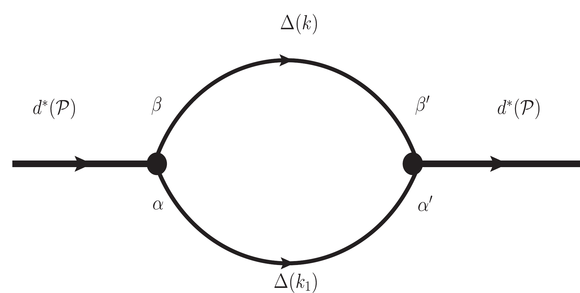
Figure 1. The mass operator of the
$ d^{*}(2380)\to\Delta\Delta. $ The explicit expression of the full mass operator can be written as
$ \begin{aligned}[b] \Sigma_{{\Delta}}^{(\mu_i'), (\mu_j)}({\cal P}) =& \big| g_{{d^*}{\Delta \Delta}}(\Lambda)\big|^2\int \frac{{\rm d}^4k}{(2\pi)^4i} \exp\Bigg (-\frac{2(k-\frac{{\cal P}}{2})_E^2}{\Lambda^2}\Bigg )\\ &\times {\rm Tr}\Bigg\{\Gamma_{\alpha'\; \; \; \beta'}^{\; (\mu_i')} \times\frac{\not k+M_{{\Delta}}}{k^2-M_{{\Delta}}^2} \Bigg (-g^{\beta\beta'}+\frac{\gamma^{\beta}\gamma^{\beta'}}{3} \\ &+ \frac{2k^{\beta}k^{\beta'}}{3M_{{\Delta}}^2}+\frac{\gamma_{\beta}k_{\beta'}-\gamma^{\beta'}k^{\beta}}{3M_{{\Delta}}} \Bigg )\times\Gamma_{\beta\; \; \; \alpha}^{\; (\mu_j)} \\ &\times\frac{\not k_1-M_{{\Delta}}}{k_1^2-M_{{\Delta}}^2}\times \Bigg (-g^{\alpha'\alpha}+\frac{\gamma^{\alpha'}\gamma^{\alpha}}{3}+ \frac{2k^{\alpha'}_{1}k^{\alpha}_{1}}{3M_{{\Delta}}^2} \\ &-\frac{\gamma^{\alpha'}k^{\alpha}_{1}-\gamma^{\alpha}k^{\alpha}_{1}}{3M_{{\Delta}}} \Bigg )\Bigg \}\Bigg |_{k_1 = {\cal P}-k}, \end{aligned} $

(7) with
$ \mu_i' $ and$ \mu_j $ being the abbreviations of$ (\mu_1',\mu_2',\mu_3') $ and$ (\mu_1,\mu_2,\mu_3) $ , respectively. In general, according to its Lorentz structure, the mass operator$ \Sigma_{(c)}^{(\mu_i'),(\mu_j)}({\cal P}) $ takes the form$ \Sigma_{(c)}^{(\mu_i'),(\mu_j)}({\cal P}) = \sum\limits_{l = 1}^8 L^{(\mu_i'), (\mu_j)}_{(l),(c)}\Sigma^{(l)}_{(c)}({\cal P}^2),\, $

(8) with
$ \Sigma^{(l)}_{(c)}({\cal P}^2) $ being the structural integrals appeared in the expression of the full mass operator, and the Lorentz structures being$ \begin{aligned}[b] L^{(\mu_i'), (\mu_j)}_{(1)} = &\frac{1}{6}\big [g^{\mu_1'\mu_1} \big (g^{\mu_2'\mu_2}g^{\mu_3'\mu_3}+g^{\mu_2'\mu_3}g^{\mu_3'\mu_2}\big )\\&+g^{\mu_1'\mu_2} \big (g^{\mu_2'\mu_1}g^{\mu_3'\mu_3}+g^{\mu_2'\mu_3}g^{\mu_3'\mu_1}\big )\\ & +g^{\mu_1'\mu_3}\big (g^{\mu_2'\mu_2}g^{\mu_3'\mu_1}+g^{\mu_2'\mu_1}g^{\mu_3'\mu_2}\big )\big ]\,,\\ = &\frac16 \big [g^{\alpha_1\beta_1}(g^{\alpha_2\beta_2}g^{\alpha_3\beta_3}+g^{\alpha_2\beta_3}g^{\alpha_3\beta_2})+......\big ] \end{aligned} $

(9) with
$ \alpha_i\in (\mu_1',\mu_2',\mu_3') $ and$ \beta_j\in (\mu_1,\mu_2,\mu_3) $ ,$ L^{(\mu_i'), (\mu_j)}_{(2)} = \frac19\big [g^{\alpha_1\alpha_2}\big (g^{\alpha_3\beta_1}g^{\beta_2\beta_3}+g^{\alpha_3\beta_2}g^{\beta_3\beta_1} +g^{\alpha_3\beta_3}g^{\beta_1\beta_2}\big )+......\big ]\,, $

(10) $ L^{(\mu_i'), (\mu_j)}_{(3)} = \frac{1}{18}\big [{{\cal P}}^{\alpha_1}{{\cal P}}^{\beta_1} \big (g^{\alpha_2\beta_2}g^{\alpha_3\beta_3}+g^{\alpha_2\beta_3}g^{\alpha_3\beta_2}\big )+...... \big ]\,, $

(11) $ L^{(\mu_i'), (\mu_j)}_{(4)} = \frac19\big [{{\cal P}}^{\alpha_1}{{\cal P}}^{\beta_1}\big (g^{\alpha_2\alpha_3}g^{\beta_2\beta_3}\big )+...... \big ]\,, $

(12) $ \begin{aligned}[b] L^{(\mu_i'), (\mu_j)}_{(5)} = &\frac{1}{18}\big [{{\cal P}}^{\alpha_1}{{\cal P}}^{\alpha_2}\big (g^{\alpha_3\beta_1}g^{\beta_2\beta_3}+ g^{\alpha_3\beta_2}g^{\beta_1\beta_3}\\ &+g^{\alpha_3\beta_3}g^{\beta_1\beta_2}\big )+...... +{{\cal P}}^{\beta_1}{{\cal P}}^{\beta_2}\big (g^{\alpha_1\beta_3}g^{\alpha_2\alpha_3}\\ &+ g^{\alpha_2\beta_3}g^{\alpha_2\alpha_3}+g^{\alpha_3\beta_3}g^{\alpha_1\alpha_2}\big )+......\big ]\,, \end{aligned} $

(13) $ L^{(\mu_i'), (\mu_j)}_{(6)} = \frac{1}{9}\big [{{\cal P}}^{\alpha_1}{{\cal P}}^{\alpha_2}{{\cal P}}^{\beta_1}{{\cal P}}^{\beta_2}\big (g^{\alpha_3\beta_3}\big )+...... \big ]\,, $

(14) $\begin{aligned}[b] L^{(\mu_i'), (\mu_j)}_{(7)} =& \frac{1}{6}\big [{{\cal P}}^{\alpha_1}{{\cal P}}^{\alpha_2}{{\cal P}}^{\alpha_3}{{\cal P}}^{\beta_1}\big (g^{\beta_2\beta_3}\big )\\&+ {{\cal P}}^{\beta_1}{{\cal P}}^{\beta_2}{{\cal P}}^{\beta_3}{{\cal P}}^{\alpha_1}\big (g^{\alpha_2\alpha_3}\big )+......\big ]\,,\end{aligned}$

(15) $ L^{(\mu_i'), (\mu_j)}_{(8)} = {{\cal P}}^{\mu_1'}{{\cal P}}^{\mu_2'}{{\cal P}}^{\mu_3'}{{\cal P}}^{\mu_1}{{\cal P}}^{\mu_2}{{\cal P}}^{\mu_3}. $

(16) Clearly, due to the property of the polarization vector of spin-3 particles, like
$ \epsilon_{\mu_1\mu_2\mu_3}({{\cal P}},\lambda) $ shown in Ref. [26], only the first term on the right-hand side of Eq. (8) gives a contribution while the other terms do not. We introduce the Lorentz projector$ \begin{aligned}[b] T_{\perp}^{(\mu_i'),(\mu_j)} =& \frac{1}{42} \big [{{\tilde g}}^{\mu_1'\mu_1}\big ({{\tilde g}}^{\mu_2'\mu_2}{{\tilde g}}^{\mu_3'\mu_3}+{{\tilde g}}^{\mu_2'\mu_3}{{\tilde g}}^{\mu_3'\mu_2}\big )\\ &+{{\tilde g}}^{\mu_1'\mu_2}\big ({{\tilde g}}^{\mu_2'\mu_1}{{\tilde g}}^{\mu_3'\mu_3}+{{\tilde g}}^{\mu_2'\mu_3}{{\tilde g}}^{\mu_3'\mu_1}\big )\\& +{{\tilde g}}^{\mu_1'\mu_3}\big ({{\tilde g}}^{\mu_2'\mu_2}{{\tilde g}}^{\mu_3'\mu_1}+{{\tilde g}}^{\mu_2'\mu_1}{{\tilde g}}^{\mu_3'\mu_2}\big )\big ]\\ & -\frac{1}{105}\big [{{\tilde g}}^{\mu_1'\mu_2'}\big ({{\tilde g}}^{\mu_3'\mu_1}{{\tilde g}}^{\mu_2\mu_3} +{{\tilde g}}^{\mu_3'\mu_2}{{\tilde g}}^{\mu_1\mu_3}+{{\tilde g}}^{\mu_3'\mu_3}{{\tilde g}}^{\mu_1\mu_2}\big )\\ & +{{\tilde g}}^{\mu_1'\mu_3'}\big ({{\tilde g}}^{\mu_2'\mu_1}{{\tilde g}}^{\mu_2\mu_3} +{{\tilde g}}^{\mu_2'\mu_2}{{\tilde g}}^{\mu_1\mu_3}+{{\tilde g}}^{\mu_2'\mu_3}{{\tilde g}}^{\mu_1\mu_2}\big )\\ &+{{\tilde g}}^{\mu_2'\mu_3'}\big ({{\tilde g}}^{\mu_1'\mu_1}{{\tilde g}}^{\mu_2\mu_3} +{{\tilde g}}^{\mu_1'\mu_2}{{\tilde g}}^{\mu_1\mu_3}+{{\tilde g}}^{\mu_1'\mu_3}{{\tilde g}}^{\mu_1\mu_2}\big )\big ]\,, \end{aligned} $

(17) with
$ {{\tilde g}}^{\mu\nu} = g_{\perp}^{\mu\nu} = -g^{\mu\nu}+\frac{{\cal P}^{\mu}{\cal P}^{\nu}}{M^2_{{d^*}}}. $

(18) It satisfies following relations
${\cal P}_iT_{\perp}^{(\mu_i'),(\mu_j)} = 0, \; \; \; \; \mu_i'\in (\mu_1',\mu_2',\mu_3')\; \rm{or}\; \mu_j\in (\mu_1,\mu_2,\mu_3), $

(19) $ L_{(\mu_i'), (\mu_i)}^{(1)}T_{\perp}^{(\mu_i'),(\mu_j)} = 1, $

(20) and
$ L_{(\mu_i'), (\mu_j)}^{(i)}T_{\perp}^{(\mu_i'),(\mu_j)} = 0,\; \; \; \; \; (i = 2,3,...,8). $

(21) Thus, when the full mass operator
$ \Sigma^{(\mu_i'),(\mu_j)}({\cal P}) $ acts with the Lorentz projector$ T_{\perp}^{(\mu_i'),(\mu_j)} $ , the product gives the scalar function$ \Sigma^{(1)}({\cal P}^2) $ in Eq. (4), and it will contribute to the compositeness condition. Finally the coupling constant$ |g|^2_{_{{d^*}\Delta\Delta}} $ can be determined from Eq. (5).It should be stressed that here we have adopted the Gaussian-type correlation function of Eq. (3),
$ \tilde\Phi(-p^2) = $ $ \exp(p^2/\Lambda^2) $ , where the model-dependent parameter Λ relates to the size of the system in the non-relativistic approximation, at least in physical meaning. Thus, one may roughly connect b, representing the size of the$ {d^*} $ in the non-relativistic wave function, to the parameter Λ by$ {b^2}/{2}\sim {1}/{\Lambda^2} $ . According to the quark model calculation in Ref. [14],$ b\sim 0.8 $ fm, and we choose the parameter value$ \Lambda\sim 0.34 $ GeV. -
There are only a few experiments of the
$ p\bar{p}\to $ $ \Delta(1232)\bar{\Delta}(1232) $ process in the literature [53-57]. Refs. [56, 57] studied$ p\bar{p}\to \Delta\bar{\Delta} $ at$ 7.23 $ and$ 12 \; {\rm GeV}$ . The samples were obtained from the large exposures of the 2-m hydrogen bubble-chamber (HBC) experiment to the U5 antiproton beam at CERN. The account of$ p\bar{p}\pi^+\pi^- $ was thought to come dominantly from the$ {\Delta}^{++}\overline{{\Delta}^{++}} $ channel. It was believed that the process can be described by the t-channel pion or reggeized pion exchange. A good description of the mass and t-distributions for the reaction at$ 3.6$ and$ 5.7\; {\rm GeV} $ was given by the one-pion exchange model [58]. Moreover, the cross section of the process, in terms of the Mandelstam variable of s, is parameterized as$ \sigma (s) = As^{-n} $ with$ A = (67\pm 20)\; {\rm mb} $ and$ n = 1.5\pm 0.1 $ [56].This
$ p\bar{p}\to \Delta\bar{\Delta} $ process can also be estimated theoretically by using an effective Lagrangian [59]$ {\cal L}^{(t_{z}^{\Delta}t_z^N)}_{\pi N\Delta} = g_{_{\pi N\Delta}}F(p_t)\bar{{\Delta}}_{\mu}^{(t_z^{{\Delta}})}\vec{\cal I}_{t_z^{{\Delta}}t_z^{N}}\cdot\partial^{\mu} \vec{\pi}^{(t_z^{\pi})}N^{(t_z^{N})}\; +\; {\rm h.c.}, $

(22) where
$ g_{_{\pi N\Delta}} $ and$ F(p_t) $ are the effective coupling constant and phenomenological form factor, respectively, the latter function is chosen to be$ F(p_t) = \Bigg(\frac{\Lambda_M^{*2}-m_{\pi}^2}{\Lambda_M^{*2}-p_t^2}\Bigg )^n\exp(\alpha p_t^2), $

(23) with the parameters
$ \Lambda_M^{*}\sim 1\; {\rm{GeV}} $ and$ n = 1 $ . In Eq. (22),$ \vec{\cal I}_{t_z^{{\Delta}}t_{z}^{N}} = C_{1t_{\pi},1/2t_z^N}^{3/2t_z^{{\Delta}}}\hat{e}^*_{t_{\pi}} $ is the isospin transition operator. Then, the cross section is$\begin{aligned}[b] \sigma =& \int\frac{(2\pi)^4\delta^4(p_1+p_2-p_3-p_4)}{4\sqrt{(p_1\cdot p_2)-m_1^2m_2^2}}\\& \times \sum\limits_{\rm Pol.}\Big |\overline{\cal M}_{if}\Big |^2\frac{{\rm d}^3p_3}{(2\pi)^32E_{p_3}}\frac{{\rm d}^3p_4}{(2\pi)^32E_{p_4}}, \end{aligned} $

(24) where
$ p_{1,2} $ (or$ p_{3,4} $ ) are the momenta of the incoming (or outgoing) particles,$ \big |\overline{\cal M}_{if}\big |^2 $ stands for averaging over the polarizations of the initial states and summing over the polarizations of final states. We can write the matrix element$ \overline{\cal M}_{if} $ , representing the contribution of the tree-diagram to$ p\bar{p}\to \Delta^{++}\overline{{\Delta}^{++}} $ , via π exchange with the Lagrangian of Eq. (22), as$\begin{aligned}[b] {\cal M}_{if}^{p\bar{p}\to {\Delta}^{++}\overline{{\Delta}^{++}}} =& g^2_{\pi N\Delta}F^2(p_t)\Big [\bar{U}^{{\Delta}}_{\alpha}p_t^{\alpha}u(p_1)\Big ] \\&\times\frac{1}{p_t^2-m_{\pi}^2}\Big [\bar{v}(p_2)p_t^{\beta}V^{{\Delta}}_{\beta}(p_4)\Big ]. \end{aligned} $

(25) The resultant cross section is shown and compared with the parameterized empirical cross section in Fig. 2. It should be mentioned that in Ref. [60]
$ F_{{\pi N\Delta}} = f_{{\pi N\Delta}}/m_{\pi} $ , and in order to fit the decay width of$ {\Delta}\to \pi N $ , where the initial momentum of Δ is set to be zero, the value of$ f_{{\pi N{\Delta}}} $ is taken as$ 2.2\pm 0.04 $ . Thus, their$ F_{{\pi N{\Delta}}}\sim (15.7\pm 0.285)\; $ GeV-1. In our present numerical calculation, to fit the parameterized cross section, we introduce an additional trajectory function$ \exp(0.2t) \; (p_t^2 = t\; <\; 0)$ and take$F_{{\pi N\Delta}}\sim 10.75 {\rm{GeV}}$ -1. Here, we find that the 10% variation in$ F_{{\pi N\Delta}} $ may cause about 50% change in the total cross section since the cross section is proportional to$ F^4_{{\pi N{\Delta}}} $ . In addition, the change of the estimated$ \sqrt{s} $ -dependent cross section with respect to the variations of the parameters$ \Lambda^*_M $ and α are shown in this figure as well. Those curves show that the cross section with smaller$ \sqrt{s} $ becomes larger when$ \Lambda^*_M $ deceases or α increases. The combined effect of$ \Lambda^*_M $ and α on the cross section, namely the effect of the phenomenological form factor, is more pronounced in the small$ \sqrt{s} $ region. Therefore, the current Lagrangian is flexible enough to fit the experimental data. It should be mentioned that in this calculation, we only consider the one-pion exchange, insert a phenomenological form factor, and take the coupling of$ F_{{\pi N\Delta}} $ as a free parameter. It seems that our tree diagram result is reasonable to reproduce the total cross section of$ p\bar{p}\to {\Delta}^{++}\overline{{\Delta}^{++}} $ , although we do not consider the contributions from other meson exchanges, for instance the ρ meson. In conclusion, the effective Lagrangian$ {\cal L}^{(t_{z}^{\Delta}t_z^N)}_{\pi N\Delta} $ mentioned above is appropriate for describing the cross section of the$ p\bar{p}\to \Delta\bar{\Delta} $ process, so it should also be acceptable and reasonable to be further used in the investigation of the$ d^*\bar{d^*} $ generation in the$ p\bar{p}\to\Delta\bar{\Delta}\to {d^*}\bar{{d^*}} $ process.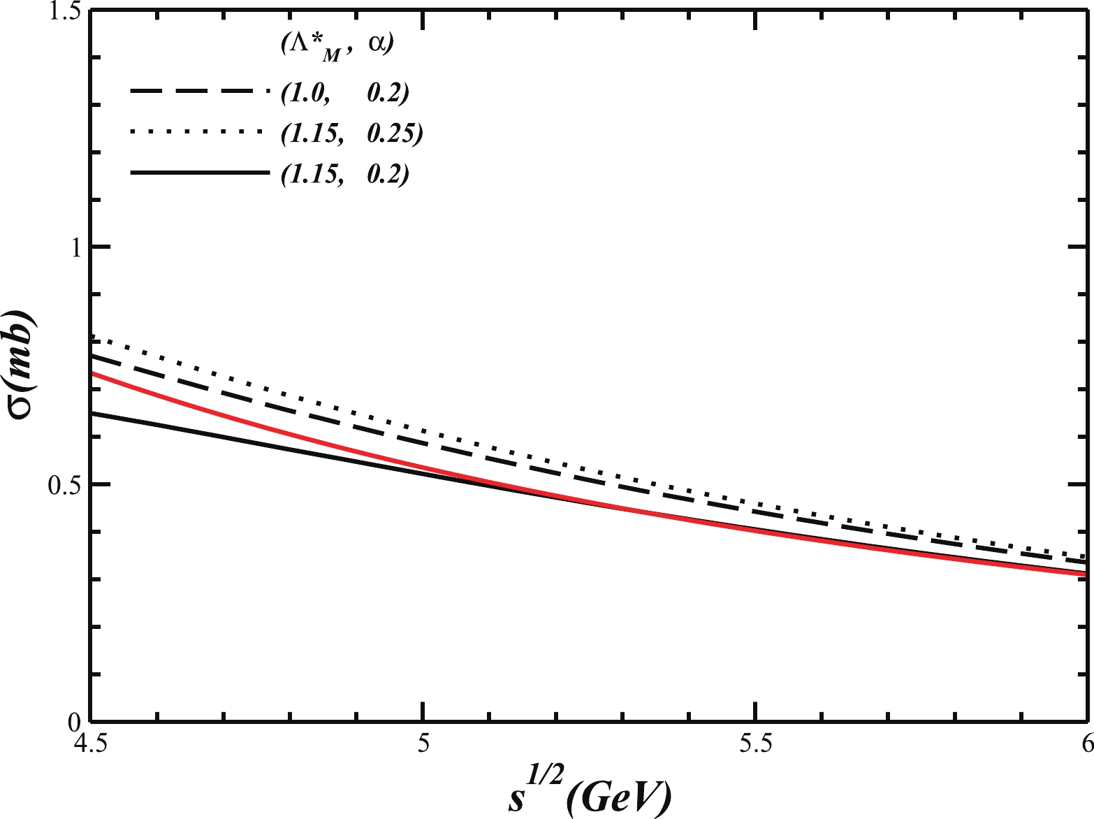
Figure 2. (color online) Estimated cross sections for
$ p\bar{p} \to\Delta^{++}\overline{\Delta^{++}} $ compared to that with a parameterized form of$ \sigma (\text{mb}) = 67s^{-1.5} $ (red curve). The black solid, dashed, and dotted curves represent the calculated results with the parameters of$ (\lambda^*_{M}({\rm GeV}),\alpha({\rm GeV}^2)) $ being (1.15, 0.2), (1.0, 0.2), and (1.15, 0.25), respectively. -
The Feynman diagram of the
$ p\bar{p}\to {d^*}\bar{{d^*}} $ process via$ \Delta\bar{{\Delta}} $ intermediate is shown in Fig. 3. In this diagram,$ {d^*}\bar{{d^*}} $ pair is generated from the$ p\bar{p}\to\Delta\bar{\Delta} $ annihilation reaction. It should be noted that in the loop, in the higher order approximation, when$ p\bar{p} $ annihilation generates a$ \Delta\bar{\Delta} $ pair, it can also create a corresponding$ C\bar{C} $ pair, therefore, when Δ interacts with Δ (or$ \bar{\Delta} $ interacts with$ \bar{\Delta} $ ), a corresponding hidden-color component$ CC $ (or$ \bar{C}\bar{C} $ ) would exist. According to the conclusion in our previous quark model calculations, about 1/3 of$ \Delta\Delta $ ($ \bar{\Delta}\bar{\Delta} $ ) and 2/3 of CC ($ \bar{C}\bar{C} $ ) can form a$ d^* $ ($ \bar{d^*} $ ), as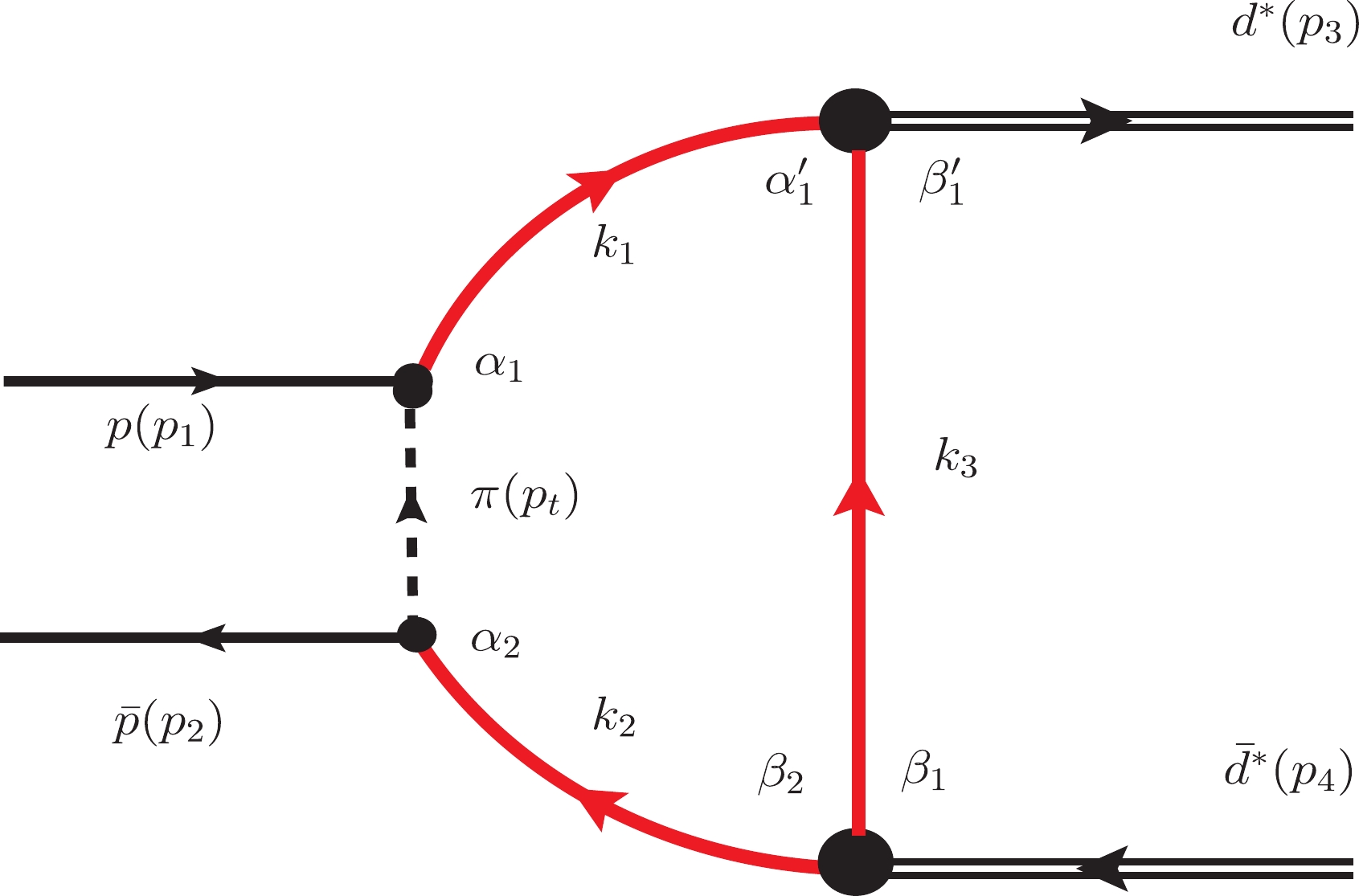
Figure 3. (color online) Feynman diagram for the
$ p\bar{p}\to d^*(2380)+\bar{d}^*(2380) $ process, where the red bold line and black double line stand for the internal Δ (or$ {\Delta}^C $ ) field and the outgoing$ {d^*} $ , respectively.$ |{d^*}>\sim \sqrt{\frac{1}{3}}|{\Delta \Delta}>+\sqrt{\frac{2}{3}}|CC>, $

with the spin and isospin quantum numbers of the colored cluster C being 3/2 and 1/2. Thus, to estimate events of
$ {d^*} $ ($ \bar{{d^*}} $ ) creation, we can only use 1/3 of the$ \Delta\Delta $ ($ \bar{\Delta}\bar{\Delta} $ ) component, because it corresponds to one$ d^* $ ($ \bar{d^*} $ ). It should be further stressed that the process in this diagram can occur only when the Mandelstam variable satisfies$ \sqrt{s}>2M_{{d^*}}\sim 4.8\; {\rm GeV} $ . It is clear that the threshold of this production channel is lower than the upper limit of the CM energy of the$ {\bar{{\rm{P}}}} $ anda device.To calculate the matrix element of Fig. 3, we have to use the vertices of
$ {\cal L}_{\pi N\Delta} $ in Eq. (22) and$ {\cal L}_{{d^*}\Delta\Delta} $ in Eq. (1). The matrix element of$ {\cal M}_{if} $ for the process of$ p\bar{p}\to{d^*}\bar{{d^*}} $ reads$ \begin{aligned}[b] M_{if}^{(p\bar p \to {d^*}\overline {{d^*}} )} =& {\bar v_N}({p_2}){\Pi _{({\nu _i}),({\mu _j})}}{u_N}({p_1}){({d^*}({p_3}))^{({\mu _j})}}\\&\times(\lambda ){({\bar d^*}({p_4}))^{({\nu _i})}}(\bar \lambda ), \end{aligned}$

(26) with
$ \begin{aligned}[b] \Pi_{(\nu_i),(\mu_j)} = &\int\frac{{\rm d}^4p_t}{(2\pi)^4i}p_t^{\alpha_2}S^C_{3/2,(\alpha_2\beta_2)}(k_2)\Gamma^{\;\beta_2,\;\;\,\beta_1}_{\;\;\;\;(\nu_i)} S^C_{3/2,(\beta_1\beta_1')}(k_3) \\ &\times \Gamma^{\;\beta'_1,\;\;\,{\alpha'_1}}_{\;\;\;\;(\mu_{j})}S_{3/2,({\alpha'}_{1}{\alpha}_1)}(k_1)p_{t}^{\alpha_1}\frac{F^2(p_t)}{p_t^2-m_{\pi}^2} \\ & \times \exp\Bigg [-\Bigg (\frac{(k_1-k_3)^2_E}{4\Lambda^2}+\frac{(k_2-k_3)_E^2}{4\Lambda^2}\Bigg )\Bigg ]\times C_{\rm Iso}, \end{aligned} $

(27) where the exponential factors in the last bracket on the right side of Eq. (27) come from the consideration of the phenomenological bound state problem of
$ {d^*} $ discussed explicitly in Sec. II, and the subscripts "E" and "M" denote "Euclidean" and "Minkowski", respectively. The propagators of a spin-3/2 particle Δ and its charge conjugate are$ \begin{aligned}[b] S_{3/2,\; \mu\nu}(p,M_{{\Delta}}) = &(\not p-m)^{-1} \\& \times \Bigg(-g_{\mu\nu}+\frac{\gamma_\mu\gamma_\nu}{3} +\frac{2p_\mu p_\nu}{3M_{{\Delta}}^2} +\frac{\gamma_\mu p_\nu-\gamma_\nu p_\mu}{3M_{{\Delta}}}\Bigg ) \,,\\ S^C_{3/2,\nu\mu}(p,M_{{\Delta}}) = & CS^{T}_{3/2,\mu\nu}(p,M_{{\Delta}}) C \,, \end{aligned} $

(28) with the charge conjugate operator being
$ C = {\rm i}\gamma^2\gamma^0 $ . Moreover, the constant$ C_{\rm Iso.} = {7}/{18} $ represents the isospin factor since the intermediate state can be either$ {\Delta}^{++}\overline{{\Delta}^{++}} $ , or$ {\Delta}^+\overline{{\Delta}^+} $ , or$ {\Delta}^0\overline{{\Delta}^0} $ (here we only consider the pion-exchange in the$ p\bar{p}\to {\Delta}\bar{{\Delta}} $ process). Then, the cross section of such a process is formally expressed by Eq. (24), where the matrix element is replaced by$ {\cal M}_{if}^{(p\bar{p}\to{d^*}\bar{{d^*}})} $ given in Eq. (26). Notice that the square of the matrix element is proportional to$ g^4_{{d^*}{\Delta \Delta}} $ and$ g^4_{{\pi N{\Delta}}} $ , respectively. Here, since the$ {d^*} $ is a spin-3 particle, its field can be described by a traceless rank-3 polarization vector like$ \epsilon_{\mu_1\mu_2\mu_3}({{\cal P}},\lambda) $ . This polarization vector has the properties of$ \epsilon_{\alpha\alpha\beta} = 0 $ ,$ \epsilon_{\alpha\beta\gamma} = \epsilon_{\beta\alpha\gamma} $ , and$ {{\cal P}}^{\alpha}\epsilon_{\alpha\beta\gamma} = 0 $ . Therefore, in the summation calculation, we have$ \begin{aligned}[b] \sum\limits_{pol.}\epsilon_{\mu\nu\sigma}\epsilon^*_{\alpha\beta\gamma} = &\frac16\Big [{\tilde g}_{\mu\alpha}\Big ({\tilde g}_{\nu\beta}{\tilde g}_{\sigma\gamma} +{\tilde g}_{\nu\gamma}{\tilde g}_{\sigma\beta}\Big ) +{\tilde g}_{\mu\beta}\Big ({\tilde g}_{\nu\alpha}{\tilde g}_{\sigma\gamma} +{\tilde g}_{\nu\gamma}{\tilde g}_{\sigma\alpha}\Big ) \\&+{\tilde g}_{\mu\gamma}\Big ({\tilde g}_{\nu\alpha}{\tilde g}_{\sigma\beta} +{\tilde g}_{\nu\beta}{\tilde g}_{\sigma\alpha}\Big ) \Big ]\\ & -\frac{1}{15}\Big [{\tilde g}_{\mu\nu}\Big ({\tilde g}_{\sigma\alpha}{\tilde g}_{\beta\gamma} +{\tilde g}_{\sigma\beta}{\tilde g}_{\alpha\gamma} +{\tilde g}_{\sigma\gamma}{\tilde g}_{\alpha\beta}\Big )\\& +{\tilde g}_{\mu\sigma}\Big ({\tilde g}_{\nu\alpha}{\tilde g}_{\beta\gamma} +{\tilde g}_{\nu\beta}{\tilde g}_{\alpha\gamma} +{\tilde g}_{\nu\gamma}{\tilde g}_{\alpha\beta}\Big )\\ & +{\tilde g}_{\nu\sigma}\Big ({\tilde g}_{\mu\alpha}{\tilde g}_{\beta\gamma} +{\tilde g}_{\mu\beta}{\tilde g}_{\alpha\gamma} +{\tilde g}_{\mu\gamma}{\tilde g}_{\alpha\beta}\Big ) \Big ], \end{aligned} $

(29) with
$ {\tilde g}_{\mu\nu} $ showed in Eq. (18). -
In this work, we employ our phenomenological effective Lagrangian approach to describe the spin-3 resonance
$ {d^*} $ . Consequently, the Feynman diagram of Fig. 3 can be calculated covariantly and relativistically. In the calculation, there is only one unique model parameter Λ. We fix this parameter according to the qualitative conclusions obtained from the dynamical calculation in the non-relativistic constituent quark model [14, 15]: (1)$ {d^*} $ contains two components$ |\Delta\Delta> $ and$ |CC> $ with probabilities$ 1/3 $ and 3/2, respectively; (2)$ {d^*} $ is a compact system with a size about$ b\sim 0.8\; {\rm fm} $ ; and (3) In the quark model approach, the strong decay widths of$ {d^*} $ , in the leading order approximation, are dominantly contributed by the$ \Delta\Delta $ component. Thus,$ \Lambda^2 \sim {2}/{b^2} $ , which gives$ \Lambda \sim 0.34\; {\rm GeV} $ when$ b\sim 0.8\; {\rm fm} $ . Further taking$ P_{\Delta\Delta} \sim 1/3 $ , we can calculate the coupling constant of$ {d^*} $ to$ \Delta\Delta $ using the formulas shown in section 2. The result shows$ g_{{d^*}\Delta\Delta}\sim 3.35 $ . We present the change of the dimensionless coupling constant$ g_{{d^*}} = g_{{d^*}\Delta\Delta}\big /\sqrt{P_{\Delta\Delta}} $ with respect to the variation of the model parameter Λ in the region of$ [0.25,\; 0.45]\; {\rm GeV} $ in Fig. 4.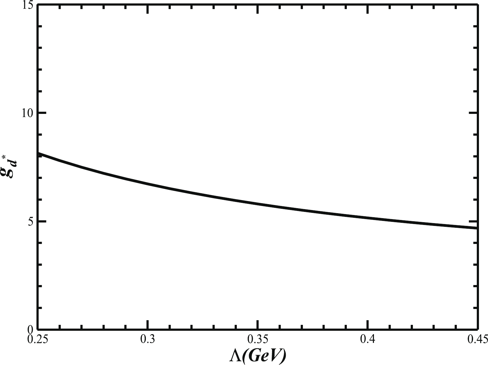
Figure 4.
$g_{{d^*}} = g_{{d^*}\Delta\Delta}\big /\sqrt{P_{\Delta\Delta}}$ in PELA versus$\Lambda \in [0.25,\; 0.45]\; {\rm GeV}.$ The curve in Fig. 4 shows that the dimensionless coupling
$ g_{{d^*}} $ relates to the model parameter Λ and to the integral of the mass operator structure. When Λ increases, the integral of the loop structure increases, and consequently the obtained$ g_{{d^*}} $ decreases. In addition, although$ g_{d^*} $ does not depend on$ P_{\Delta\Delta} $ ,$ g_{{d^*}\Delta\Delta} $ is proportional to the square root of the channel probability$ \sqrt{P_{\Delta\Delta}} $ . Finally, we would mention that we cannot dynamically determine the size parameter as well as the probability in this approach. Instead, to proceed with the calculation without contradicting the results given by the quark model, we simply borrow the corresponding qualitative conclusions given in those dynamic quark model calculations. -
In the CM energy region
$ \sqrt{s}\in[4.8-5.5]\; {\rm GeV} $ , the evaluated total cross section of the process$ p\bar{p}\to\Delta\bar{\Delta}\to $ $ {d^*}\bar{{d^*}} $ , shown by the Feynman diagram in Fig. 3, is given in Fig. 5. Here, we reiterate that the cross section is evaluated based on the qualitative interpretations of$ {d^*} $ in the non-relativistic quark model approach, with which all observed properties of$ {d^*} $ can be well described. The cross section curve in Fig. 5 tells us that the total cross section in the$ d^*\bar{d^*} $ pair production process is about 4–6 orders of magnitude smaller than that in the$ p\bar{p}\to\Delta\bar{\Delta} $ reaction.
Figure 5. (color online) Estimated cross section for the reaction of
$ p\bar{p}\to {d^*}{\bar{d}^*} $ in units of$ (\rm nb). $ We know that the cross section in Fig. 5 is dependent on the phase space as well as the matrix element
$ {\cal M}_{if} $ . The phase space increases with the increasing$ \sqrt{s} $ . The matrix element of$ {\cal M}_{if} $ relates to model parameter Λ as well as to$ \sqrt{s} $ . The estimated total cross section of$ p\bar{p}\to\Delta\bar{\Delta}\to {d^*}\bar{{d^*}} $ is also subject to the impact of the interpretation of the$ {d^*} $ state, namely its size and the probability of its$ \Delta\Delta $ component. The resultant cross section (with a fixed value of$ P_{\Delta\Delta}\sim 1/3 $ ) in Fig. 5 shows its dependence on Λ. Actually the coupling$ g_{{d^*}{\Delta \Delta}} $ is proportional to$ \sqrt{P_{\Delta\Delta}} $ and the matrix element$ {\cal M}_{if} $ is proportional to$ P_{\Delta\Delta} $ . Thus, the obtained cross section changes with respect to$ P^{2}_{\Delta\Delta} $ . Moreover, the coupling$ g_{{d^*}{\Delta \Delta}} $ and the matrix element$ {\cal M}_{if} $ are closely related to the structure of the mass operator in the structural integral and to the loop calculations of Fig. 3, respectively. Here, we only display the Λ dependence explicitly in Fig. 5. It shows that in the small$ \sqrt{s} $ region, say less than$ 5.2\; {\rm GeV} $ , the cross section is distinctly suppressed, because the coupling constant$ g_{d^*} $ decreases due to the increase of Λ. However, when$ \sqrt{s} $ is greater than$ 5.5\; {\rm GeV} $ , the production cross section with a smaller Λ value, say less than$ 0.34\; {\rm GeV} $ , may increase dramatically with the increase of$ \sqrt{s} $ due to the larger structural integral, caused by a larger Λ-dependent$ g_{{d^*}{\Delta \Delta}} $ value, and a larger phase space. It should be reiterated that as a rough estimate, we only consider the production cross section for the$ {d^*} $ –$ \bar{{d^*}} $ pair in this paper, and do not take the complicated background contribution into account. When the CM energy is about$ 5.2\; {\rm GeV} $ , the Λ dependence of the cross section becomes small, and the estimated cross section becomes significant.It should be noted that the obtained cross section of
$ p\bar{p}\to\Delta\bar{\Delta}\to {d^*}\bar{{d^*}} $ is in the order of$\text{nb}$ . According to the designed luminosity and integrated luminosity of$ {\bar{{\rm{P}}}} $ anda, which are about$ \sim 2\times 10^{32}\;{\rm cm}^{-2}/{\rm s} $ and$ \sim 10^{4}\; $ $ {\rm nb}^{-1}/{\rm day} $ , respectively, we expect that about$ (0.51, 0.71, $ $ 1.19) \times 10^{4} $ $ {d^*}\bar{{d^*}} $ events can be observed per-day at$ \sqrt{s} = (5.0, 5.1, 5.2)\; {\rm GeV} $ , if the overall efficiency is 100%. On the other hand, from a technical point of view,$ {d^*} $ cannot be directly observed. Observation of$ {d^*} $ is usually achieved through the measurements of its strong decay processes, namely measuring various mesons and baryons, such as π, proton, neutron, etc., and measuring some invariant mass spectra and Dalitz plots, etc. It is noticed that the dominated decay channels of$ {d^*} $ are$ {d^*}\to d\pi\pi $ and$ {d^*}\to pn\pi\pi $ with their partial decay widths of about$ 27 $ and$ 31\; {\rm MeV} $ , respectively, which correspond to the branching ratios of about 36% and 41%, respectively. As a consequence, the possible production events of$ p\bar{p}\to{d^*}\bar{{d^*}}\to \bar{{d^*}}\,\; d\pi\pi $ (or$ p\bar{p}\to{d^*}\bar{{d^*}}\to {d^*}\,\bar{d}\pi\pi $ ) and$ p\bar{p}\to{d^*}\bar{{d^*}}\to \bar{{d^*}}\, pn\pi\pi $ (or$ p\bar{p}\to{d^*}\bar{{d^*}}\to {d^*}\, \bar{p}\bar{n}\pi\pi $ ) can roughly be estimated. They are respectively about$ ((0.18,0.21), \;(0.26,0.29),\; (0.43,0.49))\times 10^{4} $ per-day at$ \sqrt{s} = $ $ (5.0,5.1,5.2)\; {\rm GeV} $ (if the overall efficiency is assumed 100%). Finally, it should be further mentioned that in order to avoid the interference caused by the background of a large number of produced pions and nucleons, according to our previous discussion [61, 62], it may be more practical to confirm the existence of$ {d^*} $ by looking for$ \bar{{d^*}} $ via the decay channels in above brackets. -
In this work, we estimate the cross section of the
$ p\bar{p}\to\Delta\bar{\Delta}\to {d^*}\bar{{d^*}} $ reaction, which might possibly be measured at forthcoming experiments at$ \bar{\rm P} $ anda in the CM energy of$ \sqrt{s}\in [4.8, 5.5]\; {\rm GeV} $ . A relativistic and covariant phenomenological effective Lagrangian approach is employed in the practical calculation. To describe the structure of the outgoing$ {d^*}{\bar{d}^*} $ pair, qualitative conclusions from the sophisticated and dynamic calculations in the non-relativistic constituent quark model, with which all existing data can be well explained, are directly adopted to approximately fix the model parameter Λ. The estimated production cross section for$ {d^*}{\bar{d}^*} $ should be a lower bound, since in our assumption, only 1/3 of$ \Delta\Delta $ is considered to be an ingredient of$ {d^*} $ . The result shows that the estimated production cross section of this reaction is in the order of$\text{nb}$ which is much smaller than the known cross section of$ p\bar{p}\to\Delta\bar{\Delta} $ whose value is in the order of${\rm mb} $ . Nevertheless, among a huge amount of events of produced hadron pair at$ \bar{\rm P} $ anda, there may still exist a certain amount of events of produced$ {d^*}{\bar{d}^*} $ pairs. These events are expected to be observed through measuring the final baryons and mesons in some strong decay processes of$ {d^*} $ , such as$ {d^*}\to d\pi\pi $ (or$ \bar{{d^*}}\to \bar{d}\pi\pi $ ) and$ {d^*}\to pn\pi\pi $ (or$ \bar{{d^*}}\to \bar{p}\bar{n}\pi\pi $ ). We also roughly estimate the event probabilities of these processes from the branching ratios of the$ {d^*} $ strong decays as a reference. -
We would like to thank Prof. Zongye Zhang for valuable discussions.
Possible dibaryon production at ${{\overline {\bf P} }}$ anda with a Lagrangian approach
- Received Date: 2021-09-06
- Available Online: 2022-02-15
Abstract: In order to confirm the existence of the dibaryon state


 DownLoad: