


 Abstract
 HTML
HTML Reference
 Related
 PDF
PDF


-
Neutron-deficient actinide nuclei are new growing points in modern nuclear physics [1-3]. Located in the vicinity of the proton drip line, these nuclei are characterized by their large proton/neutron ratios and short half-lives. Synthesizing these nuclei is a challenging task in experimental nuclear physics. Owing to recent advances in beam facilities, detection systems, and analysis methods, a number of new neutron-deficient actinide nuclei have been synthesized since 2014, including
$ {}^{205} {\rm{Ac}}$ [4],$ {}^{211} {\rm{Pa}}$ [5],$ {}^{214,216,221} {\rm{U}}$ [3, 6],$ {}^{219,220,222-224} {\rm{Np}}$ [1, 2, 7-9],$ {}^{236} {\rm{Bk}}$ [10],$ {}^{240} {\rm{Es}}$ [10], and$ {}^{244} {\rm{Md}}$ [11]. α decay is one of the most important decay modes in these nuclei [12-21]. It is widely adopted as a powerful tool to identify new neutron-deficient actinide nuclei in experiments. The measured α-decay energies and half-lives also provide a valuable window to probe the evolution of shell structure and cluster formation in neutron-deficient actinide nuclei. In Refs. [1, 2, 7-9], the α-decay data of the new neutron-deficient Neptunium isotopes$ {}^{219,220,222-224} {\rm{Np}}$ were analyzed systematically to probe the robustness of the magic number$ N = 126 $ along the Neptunium isotopic chain. Very recently, a new neutron-deficient Uranium isotope$ {}^{214} {\rm{U}}$ was produced via the$ {}^{182}\text{W}({}^{36}\text{Ar},4n){}^{214}\text{U} $ reaction [3]. The α-decay systematics suggest that the α-cluster formation is enhanced abnormally by a factor of two in comparison with even-even nuclei with$ 84\leqslant Z\leqslant 90 $ and$ N<126 $ . The authors of Ref. [3] conjectured that such an enhancement is closely related to the strong monopole interaction between the$ \pi1f_{7/2} $ and$ \nu1f_{5/2} $ orbits. In spite of these achievements, several crucial neutron-deficient actinide nuclei remain unknown in experiments. For example, the neutron-deficient Neptunium isotope$ {}^{221} {\rm{Np}}$ is crucial for addressing the problem of the robustness of the$ N = 126 $ magic number in Neptunium completely. However, this isotope has not been produced yet. Similarly, the neutron-deficient Uranium isotope$ {}^{220} {\rm{U}}$ has not been produced in experiments as well, which is crucial for examining the robustness of the$ N = 126 $ magic number in Uranium. Reliable theoretical predictions on their α-decay properties may be important for their future synthesis and identification.On the theoretical side, many models have been proposed in the literature to predict α-decay energies and α-decay half-lives. For α-decay energies, the popular models include the finite-range droplet model (FRDM) [22], the finite-range liquid-drop model (FRLDM) [22], the Thomas-Fermi (TF) model [23], the Duflo-Zuker (DZ) model [24], the empirical formula based on the liquid-drop model [25], and the linear trajectory under the valence correlation scheme [26]. For α-decay half-lives, the popular models include the new Geiger-Nuttall law (NGNL) [27], the density-dependent cluster model (DDCM) [28-33], the multiple channel cluster model (MCCM) [34, 35], the generalized liquid drop model (GLDM) [36], the universal decay law (UDL) [37], the quartetting wave function approach [38, 39], and the quartet model [40]. These traditional methods have been adopted in various experimental works to provide theoretical values for comparison. In Ref. [41], the authors calculated the α-decay properties of some neutron-deficient actinide nuclei, including two new isotopes
$ {}^{219} {\rm{Np}}$ and$ {}^{220} {\rm{Np}}$ , using the improved Buck-Merchant-Perez cluster model. The theoretical results showed good agreement with the experimental data within a factor$ \approx $ 2. In spite of these successes, considering their physical importance, it is valuable to continue developing new models for reliable theoretical predictions on the α-decay properties.Machine learning has made tremendous progress in the past ten years and has changed our social life in a significant way. It is widely used in image recognition, product recommendation, autonomous vehicles, and email spam. Besides celebrated successes in computer science, machine learning algorithms have also been used to study realistic problems in modern physics. For example, machine learning was successfully used for estimating entropy production [42], distinguishing different topological phases [43], and detecting multimode Wigner negativity [44]. Meanwhile, machine learning has also been applied to the field of nuclear physics [45-60]. As one of the machine learning algorithms, the Gaussian process has provided new ideas for the studies of many important physical problems in recent years [61-66]. The Gaussian process is a popular machine learning algorithm because it can provide error bars for the predictive values. This advantage could help visualize the model uncertainties and quantify the theoretical uncertainties [67]. For α-decay studies, only a few calculations are available based on a machine learning algorithm called the artificial neural network [68], and the power of machine learning algorithms has not been fully realized in α-decay studies.
In this work, we propose a new model for α decay within the framework of the Gaussian process, which is an important machine learning algorithm. We use this new model to predict the α-decay energies and half-lives of some unknown neutron-deficient actinide nuclei. Our theoretical results could be useful for future experimental synthesis and identification of these isotopes. The remainder of this paper is organized as follows. In Sec. II, a brief introduction to the Gaussian process is provided. In Sec. III, the theoretical results are detailed for neutron-deficient actinide nuclei with 89
$\leqslant $ Z$\leqslant $ 94. The summary is provided in Sec. IV. -
α-decay energies and α-decay half-lives are two of the most important observables in α decay. They depend on the neutron number N, proton number Z, orbital angular momentum L of the α emitter, as well as many other physical quantities in a very complicated way. It is an important problem to calculate the α-decay energies and half-lives accurately in theoretical models. In this work, we propose the use of a machine learning algorithm called the Gaussian process to capture the complex correlations between the α-decay observables and intrinsic physical properties of α emitters. This can be implemented in three steps. In Step I, we construct our Gaussian process model under the guidance of theoretical considerations of the α-decay physics and general experience of the machine learning field. In Step II, the Gaussian process model is trained with respect to the experimental α-decay data, which are referred to as the training set in machine learning terminologies. In Step III, the trained Gaussian process model is used to calculate the α-decay properties of unknown α emitters. These results could be helpful for their synthesis and identification in future experiments.
For later convenience, we introduce a few notations used in statistics and machine learning. Let A be a set of independent random variables.
$ {\boldsymbol{A}} \sim {\cal{N}}({\boldsymbol{\mu}}, \Sigma) $ means that these random variables obey the multivariate Gaussian distribution with the mean vector given by µ and the covariance matrix given by Σ.$ {P}({\boldsymbol{B}}|{\boldsymbol{A}}) $ denotes the conditional probability distribution of B if A happens.$ \left\lbrace {\boldsymbol{X}}, {\boldsymbol{Y}} \right\rbrace $ denotes the training set with n known data points, where$ {\boldsymbol{X}} = \left[ x_1, x_2, \cdots, x_n \right]^T $ and$ {\boldsymbol{Y}} = \left[ y_1, y_2, \cdots, y_n \right]^T $ are the inputs and outputs, respectively.$ \left\lbrace {\boldsymbol{X}}_*, {\boldsymbol{Y}}_* \right\rbrace $ , with$ {\boldsymbol{X}}_* = \left[ x_{1_*}, x_{2_*}, \cdots, x_{n_*} \right]^T $ and$ {\boldsymbol{Y}}_* = \left[ y_{1_*}, y_{2_*}, \cdots, y_{n_*} \right]^T $ , denotes$ n_* $ unknown data points. The main goal of machine learning is to predict the values of the unknown outputs$ {\boldsymbol{Y}}_* $ based on the known Y.The Gaussian process is a popular nonparametric model in machine learning. It is a stochastic process based on the Gaussian distribution and is often used to study the complicated correlations between different quantities in a high-dimensional function space. It can be defined as a collection of random variables with the novel property that any finite number of them satisfies a joint Gaussian distribution [69]. Let us consider a n-dimensional function
$ {\boldsymbol{Y}}({\boldsymbol{X}}) $ with$ {\boldsymbol{X}} = \left[ x_1, x_2, \cdots, x_n \right]^T $ . If$ {\boldsymbol{Y}} = \left[ y(x_1), y(x_2), \cdots, y(x_n) \right]^T = $ $ \left[ y_1, y_2, \cdots, y_n \right]^T $ obeys a joint Gaussian distribution, the Gaussian process is given by$ {\boldsymbol{Y}}\sim{\cal{GP}}({\boldsymbol{M}}({\boldsymbol{X}}),{\boldsymbol{K}}({\boldsymbol{X}},{\boldsymbol{X}})). $

(1) Here,
$ {\cal{GP}} $ is an abstract symbol for the Gaussian process and the random variables are the function values$ y_{i} = y(x_{i}) $ at the point$ x_{i} $ . X and Y are the Gaussian process inputs and outputs, respectively.$ {\boldsymbol{M}}({\boldsymbol{X}})\; = \; [m(x_1), m(x_2), \cdots, m(x_n)]^T $ denotes the values of the mean function of the Gaussian process, and$ {\boldsymbol{K}}({\boldsymbol{X}}, {\boldsymbol{X}}) = [k(x_i, x_j)]_{n\times n} $ is the$ n\times n $ kernel function matrix of the Gaussian process. The kernel function$ k(x_i,x_j) $ captures the correlations between the Gaussian process outputs at the input points$ x_i $ and$ x_j $ . The details of the kernel function$ k(x_i,x_j) $ are introduced later. Because the marginal distribution of the multivariate Gaussian distribution is still Gaussian, Eq. (1) can be represented more clearly as$ \left[ {\begin{array}{*{20}{c}} {{y_1}}\\ \vdots \\ {{y_n}} \end{array}} \right]\sim {\cal{N}}\left( {\left[ {\begin{array}{*{20}{c}} {m({x_1})}\\ \vdots \\ {m({x_n})} \end{array}} \right],\left[ {\begin{array}{*{20}{c}} {k({x_1},{x_1})}& \cdots &{k({x_1},{x_n})}\\ \vdots & \ddots & \vdots \\ {k({x_n},{x_1})}& \cdots &{k({x_n},{x_n})} \end{array}} \right]} \right),$

(2) where
$ {\cal{N}} $ represents the Gaussian distribution. For consistency, the kernel function matrix$ {\boldsymbol{K}}({\boldsymbol{X}},{\boldsymbol{X}}) $ should be symmetric and positive semidefinite.For the α-decay studies, the Gaussian process inputs X can be the proton numbers Z, neutron numbers N, and orbital angular momenta L of different α emitters, while the Gaussian process outputs Y can be the corresponding α-decay observables, i.e., the α-decay energies and half-lives. The proton number Z and neutron number N are chosen as the features of the inputs because they are among the most important intrinsic physical properties of nuclei. In this work, the Gaussian process input is
$ x_{i} = ( Z_{i}, N_{i} ) $ for an α emitter when its corresponding output is$ y_{i} = Q_{\alpha}^\text{Expt.} $ to describe the α-decay energy for an α-decay emitter. When describing the corresponding α-decay half-lives, the Gaussian process input and output are given by$ x_{i} = ( Z_{i}, N_{i}, L_{i} ) $ and$ y_{i} = \text{log}_{10}T_{\alpha}^\text{Expt.} $ , respectively. The feature L in the input is added as traditional models show that it is crucial for calculating the unfavored α-decay half-lives [41]. Let$ \{{\boldsymbol{X}},{\boldsymbol{Y}}\} $ be the training set of the Gaussian process, which contains the experimental data of the observed α emitters. Then, under the framework of the Gaussian process, the known α-decay observables Y at the points X and unknown α-decay observables$ {\boldsymbol{Y}}_* $ at the points$ {\boldsymbol{X}}_* $ satisfy the joint Gaussian distribution$ P({\boldsymbol{Y}}, {\boldsymbol{Y}}_*) = {\cal{N}}({\boldsymbol{M}}_{**}, {\boldsymbol{K}}_{**}) $ with$ P({\boldsymbol{Y}}_*) = {\cal{N}}({\boldsymbol{M}}_*, {\boldsymbol{K}}_*) $ , whose mean vector is$ {\boldsymbol{M}}_{**} = \left[ {\boldsymbol{M}}, {\boldsymbol{M}}_* \right]^T $ and the covariance matrix$ {\boldsymbol{K}}_{**} $ is given by$ {{\boldsymbol{K}}_{{\rm{**}}}}{\rm{ = }}\left[ {\begin{array}{*{20}{c}} {{\boldsymbol{K}}({\boldsymbol{X}},{\boldsymbol{X}})\quad {\boldsymbol{K}}({\boldsymbol{X}},{{\boldsymbol{X}}_{\rm{*}}})}\\ {{\boldsymbol{K}}({{\boldsymbol{X}}_{\rm{*}}},{\boldsymbol{X}})\;{\boldsymbol{K}}({{\boldsymbol{X}}_{\rm{*}}},{{\boldsymbol{X}}_{\rm{*}}})} \end{array}} \right].$

(3) If there are a number of n points in the training set and a set of
$ n_* $ new points for the predictions,$ {\boldsymbol{K}}({\boldsymbol{X}},{\boldsymbol{X}}_*) $ and$ {\boldsymbol{K}}({\boldsymbol{X}}_*,{\boldsymbol{X}}_*) $ are the$ n\times n_* $ and$ n_*\times n_* $ matrices, respectively, and$ {\boldsymbol{K}} ( {\boldsymbol{X}}, {\boldsymbol{X}}_{*} ) = {\boldsymbol{K}} ( {\boldsymbol{X}}_*, {\boldsymbol{X}} )^T $ .To obtain a reasonable predictive distribution on
$ {\boldsymbol{Y_{*}}} $ , we are interested in the conditional distribution of$ {\boldsymbol{Y_{*}}} $ when Y is given, based on the definition of the conditional probability function$ {P}({\boldsymbol{Y}}_* | {\boldsymbol{Y}}) = \frac{{P}({\boldsymbol{Y}}, {\boldsymbol{Y}}_{*})}{{P}({\boldsymbol{Y}})}, $

(4) where
$ {P}({\boldsymbol{Y}}) = {\cal{N}}({\boldsymbol{M}}, {\boldsymbol{K}}) $ with$ {\boldsymbol{K}} = {\boldsymbol{K}} ( {\boldsymbol{X}}, {\boldsymbol{X}}) $ . After conditioning the joint Gaussian distribution, the predictive distribution on$ {\boldsymbol{Y_{*}}} $ is expressed as$ \begin{aligned}[b]& {\boldsymbol{Y_{*}}} | {\boldsymbol{Y}} \sim {\cal{N}} \big[ {\boldsymbol{M}}({\boldsymbol{X_{*}}}) + {\boldsymbol{K}}( {\boldsymbol{X}}, {\boldsymbol{X_{*}}})^T {\boldsymbol{K}}( {\boldsymbol{X}}, {\boldsymbol{X}} )^{-1} ({\boldsymbol{Y}} - {\boldsymbol{M}}({\boldsymbol{X}})), \\ &\quad{\boldsymbol{K}}( {\boldsymbol{X_{*}}}, {\boldsymbol{X_{*}}})-{\boldsymbol{K}}( {\boldsymbol{X}}, {\boldsymbol{X_{*}}})^T {\boldsymbol{K}}( {\boldsymbol{X}}, {\boldsymbol{X}})^{-1} {\boldsymbol{K}}( {\boldsymbol{X}}, {\boldsymbol{X_{*}}})\big], \end{aligned} $

(5) which is the central equation for the predictions with the Gaussian process. In this work,
$ {\boldsymbol{M}}({\boldsymbol{X}}) $ , which is the mean function for the training set, is set to zero as usual due to a lack of prior knowledge. In addition, the mean function for the prediction points, which is denoted by$ {\boldsymbol{M}}({\boldsymbol{X_{*}}}) $ , is also chosen to be zero.The kernel function
$ k(x_i,x_j) $ is crucial for the predictability of the Gaussian process. In this work, we consider three common choices:● Matérn 3/2:
$ k({x}_i,{x}_j) = \eta^2\left( 1+\frac{\sqrt{3}}{l}r_{ij}\right)\mathrm{exp}\left(-\frac{\sqrt{3}}{l}r_{ij}\right), $

● Matérn 5/2:
$ k({x}_i, {x}_j) = \eta^2\left( 1+\frac{\sqrt{5}}{l}r_{ij}+\frac{5}{3l^{2}}r_{ij}^{2}\right)\mathrm{exp}\left(-\frac{\sqrt{5}}{l}r_{ij}\right) , $

● Matérn 7/2:
$ k({x}_i, {x}_j) = \eta^2\left( 1+\frac{\sqrt{7}}{l}r_{ij}+\frac{14}{5l^{2}}r_{ij}^{2}+\frac{7\sqrt{7}}{15l^{3}}r_{ij}^{3}\right)\mathrm{exp}\left(-\frac{\sqrt{7}}{l}r_{ij}\right) , $

where
$ r_{ij}\equiv \left\| {x}_i-{x}_j \right\| $ is the distance between the input points$ x_i $ and$ x_j $ , and$ \theta\equiv\left\lbrace \eta^{2}, l\right\rbrace $ represents the hyperparameters of the Gaussian process. The free hyperparameters θ can be determined by maximizing the natural logarithm of the likelihood function$ \mathrm{ln}\,{P}\left( {\boldsymbol{Y}}|{\boldsymbol{X}}, \theta \right) = -\frac{1}{2}{\boldsymbol{Y}}^T{\boldsymbol{K}}({\boldsymbol{X}},{\boldsymbol{X}})^{-1}{\boldsymbol{Y}}-\frac{1}{2}\mathrm{ln}\left| {\boldsymbol{K}}({\boldsymbol{X}},{\boldsymbol{X}})\right|-\frac{n}{2}\mathrm{ln}(2\pi), $

(6) -
With the model discussed above, we perform predictions on the α-decay energies and half-lives for some unknown neutron-deficient actinide nuclei with 89
$\leqslant $ Z$\leqslant $ 94, respectively. To predict the α-decay energies and half-lives, the Gaussian process inputs are chosen as$ x_{i} = \left( Z_{i}, N_{i} \right) $ and$ x_{i} = \left( Z_{i}, N_{i}, L_{i} \right) $ for each nucleus, respectively. Here, the angular momentum and parity follow the conservation laws [41]$ \left|I_{f}-I_{i}\right| \leqslant L \leqslant I_{f}+I_{i},\quad \dfrac{\pi_{f}}{\pi_{i}} = (-1)^{L}, $

(7) where
$ I_{i} $ ,$ I_{f} $ ,$ \pi_{i} $ , and$ \pi_{f} $ are the spins and parities of the initial and final states, respectively. Meanwhile, the Gaussian process outputs are the corresponding α-decay energies and the common logarithm of the α-decay half-lives, respectively. Here, the Gaussian process training sets consist of, respectively, a set of 101 actinide nuclei with available experimental α-decay energies and a set of 102 actinide nuclei with available experimental α-decay half-lives (see the supplementary material). The corresponding experimental α-decay energies and half-lives are obtained from the AME2016 [71, 72] and the NUBASE2016 [73], respectively. Regarding the nuclei with newly reported α-decay properties, such as$ ^{211,220} {\rm{Pa}}$ [5, 74],$ ^{216,218,223} {\rm{U}}$ [3, 75], and$ ^{219,220,222} {\rm{Np}}$ [1, 2, 7], we select the newest experimental results as the outputs for the Gaussian process training sets, while the α-decay properties of the newest neutron-deficient nucleus$ ^{214} {\rm{U}}$ are not included. For the new experimental α-decay half-lives with asymmetric uncertainties, their uncertainties are symmetrized as in NUBASE2016 [73]. To provide the systemic error for the Gaussian process, three different kernel functions are used in this work. Table 1 shows the hyperparameters of the Gaussian process determined in this work. The first column lists the three kernel functions used for calculating both the α-decay energies and half-lives. The second and third columns list the hyperparameters for calculating the α-decay energies with different kernel functions, and the last two columns list those for calculating the α-decay half-lives. Besides, Fig. 1 depicts the natural logarithm of the likelihood function values for training the α-decay energies and half-lives over the hyperparameter space using the Gaussian process with three different kernel functions. The red stars indicate the maximum natural logarithm of the likelihood function values.kernel function $\eta^{2}_Q/\text{MeV}$ 

$ l_Q $ 

$ {\eta}^{2}_T $ 

$ l_T $ 

Matérn 3/2 34.480 17.010 22.566 5.389 Matérn 5/2 22.680 6.386 14.457 2.946 Matérn 7/2 18.594 4.199 13.020 2.381 Table 1. The hyperparameters
$ \theta_Q \equiv\left\lbrace \eta^{2}_Q, l_Q\right\rbrace $ and$ \theta_T \equiv\left\lbrace \eta^{2}_T, l_T\right\rbrace $ of the Gaussian process determined by two training sets for calculating the α-decay energies and half-lives, respectively.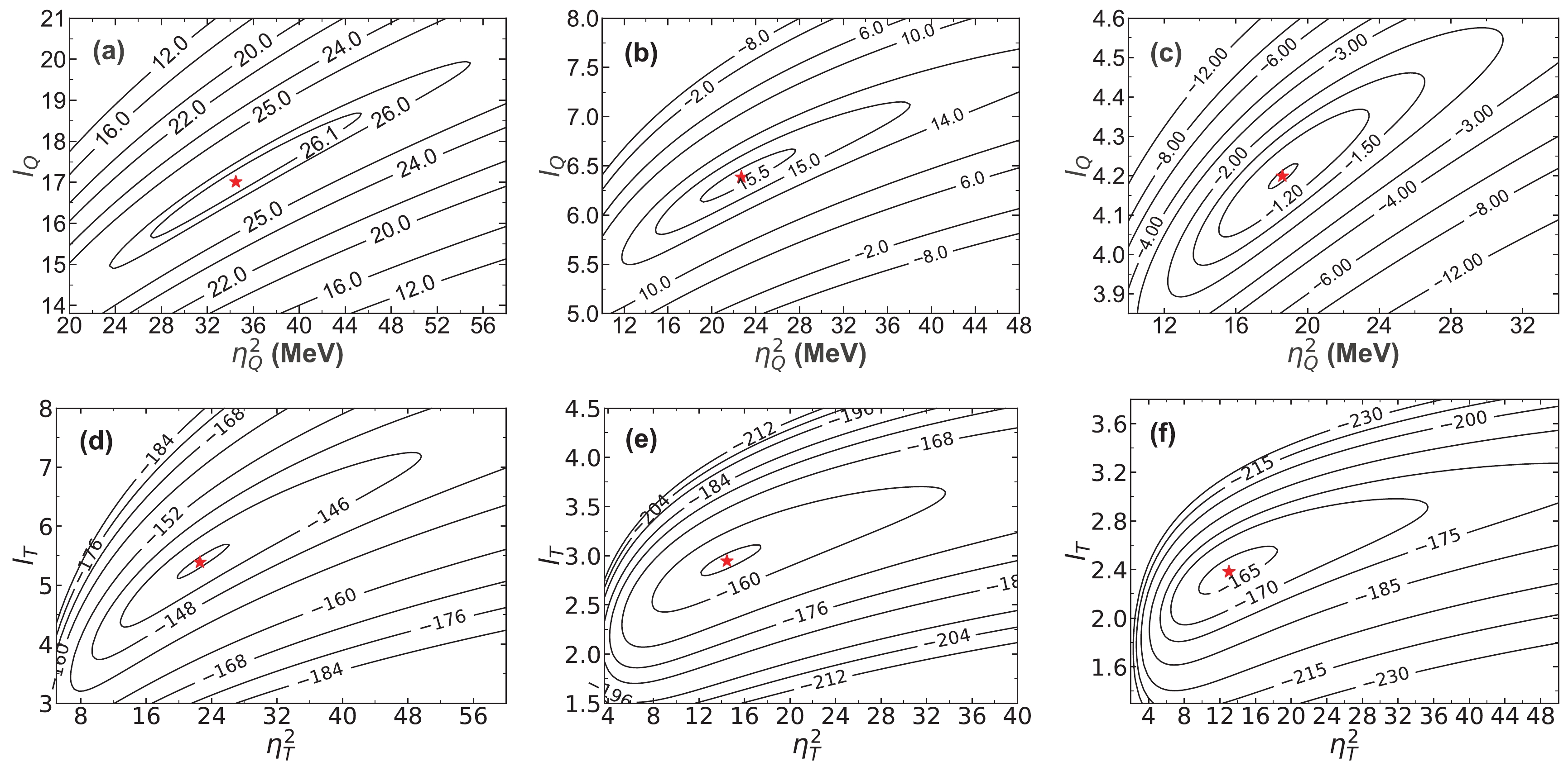
Figure 1. (color online) The natural logarithm of the likelihood function values for training the α-decay energies and half-lives over the hyperparameter space using the Gaussian process with three different kernel functions. Fig. 1(a) - (c) depict the natural logarithm of the likelihood function values over the hyperparameter space when training the α-decay energies with the Matérn 3/2, Matérn 5/2, and Matérn 7/2 kernel functions, respectively. Fig. 1(d) - (f) show, respectively, the natural logarithm of the likelihood function values for training the α-decay half-lives using the Matérn 3/2, Matérn 5/2, and Matérn 7/2 kernel functions.
We first calculate the α-decay properties of the new actinide nucleus
$ ^{214} {\rm{U}}$ to test the reliability of the Gaussian process. The predictive α-decay energies and half-lives with three kernel functions versus the neutron number for the Uranium isotopes are shown in Fig. 2. In addition, the 1σ confidence intervals provided by the Gaussian process with three kernel functions are also plotted in Fig. 2. The black dashed line represents N = 128. The α-decay energies of the new nuclei$ ^{214} {\rm{U}}$ are marked by the black arrow in Fig. 2(a). It can be clearly seen that, for$ ^{214} {\rm{U}}$ , all the α-decay energies calculated with the three kernel functions can reproduce the newest experimental results well. Numerically, the calculated α-decay energies of$ ^{214} {\rm{U}}$ are 8.679, 8.652, and 8.633 MeV using the Matérn 3/2, Matérn 5/2, and Matérn 7/2 kernel functions, respectively. In Ref. [3], the experimental α-decay energy of$ ^{214} {\rm{U}}$ is 8.696 MeV. The deviations between the experimental result and the theoretical results calculated with the Matérn 3/2, Matérn 5/2, and Matérn 7/2 kernel functions are 0.017, 0.044, and 0.063 MeV, respectively. These small deviations show that the calculated results are in good agreement with the experimental result. Besides, we applied the leave-one-out cross-validation to the Gaussian process with three Matérn kernel functions. The root mean squared errors of the Gaussian process with the Matérn 3/2, Matérn 5/2, and Matérn 7/2 kernel functions are 0.082, 0.082, and 0.100 MeV, respectively, when calculating the α-decay energies. The results indicate that the Gaussian process is a pretty good model for calculating the α-decay energies. Similarly, the α-decay half-lives of the new nuclei$ ^{214} {\rm{U}}$ are denoted by the black arrow in Fig. 2(b). It can be seen that the α-decay half-lives calculated with the Matérn 3/2, Matérn 5/2, and Matérn 7/2 kernel functions are all very close to the experimental result. The predictive results are 1.23×10⁻³, 1.28×10⁻³, and 1.37×10⁻³ s, respectively. The experimental α-decay half-life is 9.94×10$ ^{-4} $ s in Ref. [3]. Therefore, the calculated α-decay half-lives are in good accordance with the experimental result with a factor of 1.240, 1.289, and 1.376, respectively. We also performed the leave-one-out cross-validation on the Gaussian process with three Matérn kernel functions when calculating the α-decay half-lives. The root mean squared errors of the Gaussian process with the Matérn 3/2, Matérn 5/2, and Matérn 7/2 kernel functions are 0.734, 0.807, and 0.861, respectively. These deviations are acceptable due to the difficulties in calculating the α-decay half-lives. Based on the discussion above, it can be argued that the Gaussian process is a reliable method for predicting the α-decay properties. This indicates that the complex correlations between the α-decay observables and intrinsic physical properties of the α emitters can be described using the Gaussian process.
Figure 2. (color online) Predictions on (a) α-decay energies and (b) half-lives versus the neutron number for the Uranium isotopes. For (a), the black hollow squares indicate the experimental α-decay energies. The yellow upper triangles and purple lower triangles represent the α-decay energies derived from the finite-range droplet model (FRDM) [22], and those extracted from the finite-range liquid-drop model (FRLDM) [22], respectively. The green right triangles, blue left triangles, and red dots, respectively, denote the predictive α-decay energies obtained using the Matérn 3/2, Matérn 5/2, and Matérn 7/2 kernel functions. For (b), the black hollow squares represent the experimental α-decay half-lives. The yellow upper triangles represent the α-decay half-lives calculated using the new Geiger-Nuttall law (NGNL) [27] and the purple lower triangles represent the α-decay half-lives calculated using the density-dependent cluster model (DDCM) [28]. The green right triangles, blue left triangles, and red dots present the predictive α-decay half-lives obtained using the Matérn 3/2, Matérn 5/2, and Matérn 7/2 kernel functions, respectively. The predictive α-decay properties are in good accordance with those calculated with the traditional models.
We further predict the α-decay properties of some unknown neutron-deficient actinide nuclei with 89
$\leqslant $ Z$\leqslant $ 93 using the Gaussian process, and the results are shown in Table 2. To verfiy the dependability of our predictive results, we compare them with the theoretical results calculated using the traditional models. In Table 2, the first column shows the α-decay parent nuclei. The second, third, and fourth columns denote the predictive α-decay energies obtained with the Matérn 3/2, Matérn 5/2, and Matérn 7/2 kernel functions, respectively. The fifth and sixth columns list the α-decay energies extracted from the FRDM and FRLDM, respectively. The seventh, eighth, and ninth columns list the α-decay half-lives predicted using the Matérn 3/2, Matérn 5/2, and Matérn 7/2 kernel functions, respectively. The last two columns represent, respectively, the α-decay half-lives calculated using the new NGNL and DDCM. To compare the predictive α-decay results with the theoretical calculations from the traditional models more visually, all results with the 1σ confidence intervals are shown in Fig. 2 - Fig. 6.Nucl. $ Q_{M_{3/2}}/{\rm{MeV}} $ 

$ Q_{M_{5/2}}/{\rm{MeV}} $ 

$ Q_{M_{7/2}}/{\rm{MeV}} $ 

$ Q_{22a}/{\rm{MeV}} $ 

$ Q_{22b}/{\rm{MeV}}$ 

$T_{1/2}^{M_{3/2}}/{\rm{s} }$ 

$ T_{1/2}^{M_{5/2}}/{\rm{s}} $ 

$ T_{1/2}^{M_{7/2}}/{\rm{s}} $ 

$T_{1/2}^{\rm NGNL}/{\rm{s} }$ 

$T_{1/2}^{\rm DDCM}/{\rm{s} }$ 

$ ^{204} {\rm{Ac}}$ 

8.158 8.120 8.103 8.435 8.625 2.23 $ \times 10^{-1} $ 

2.65 $ \times 10^{-1} $ 

2.49 $ \times 10^{-1} $ 

1.18 $ \times 10^{-2} $ 

1.31 $ \times 10^{-2} $ 

$ ^{206} {\rm{Th}}$ 

8.374 8.302 8.199 8.515 8.715 1.39 $ \times 10^{-2} $ 

1.92 $ \times 10^{-2} $ 

2.48 $ \times 10^{-2} $ 

8.80 $ \times 10^{-3} $ 

4.14 $ \times 10^{-3} $ 

$ ^{207} {\rm{Th}}$ 

8.289 8.255 8.205 8.205 8.405 3.22 $ \times 10^{-3} $ 

3.49 $ \times 10^{-3} $ 

4.05 $ \times 10^{-3} $ 

1.17 $ \times 10^{-2} $ 

6.56 $ \times 10^{-3} $ 

$ ^{209} {\rm{Th}}$ 

8.130 8.138 8.146 7.825 8.035 2.17 $ \times 10^{-2} $ 

2.46 $ \times 10^{-2} $ 

3.04 $ \times 10^{-2} $ 

4.46 $ \times 10^{-2} $ 

2.44 $ \times 10^{-2} $ 

$ ^{210} {\rm{Pa}}$ 

8.533 8.524 8.498 8.265 8.495 2.27 $ \times 10^{-3} $ 

2.91 $ \times 10^{-3} $ 

3.58 $ \times 10^{-3} $ 

4.44 $ \times 10^{-3} $ 

4.66 $ \times 10^{-3} $ 

$ ^{222} {\rm{Pa}}$ 

8.883 8.895 8.901 8.145 8.325 $ ^{213} {\rm{U}}$ 

8.759 8.713 8.666 8.385 8.605 1.39 $ \times 10^{-3} $ 

1.59 $ \times 10^{-3} $ 

1.67 $ \times 10^{-3} $ 

2.82 $ \times 10^{-3} $ 

1.48 $ \times 10^{-3} $ 

$ ^{214} {\rm{U}}$ 

8.679 8.652 8.633 8.445 8.665 1.23 $ \times 10^{-3} $ 

1.28 $ \times 10^{-3} $ 

1.37 $ \times 10^{-3} $ 

4.09 $ \times 10^{-3} $ 

1.70 $ \times 10^{-3} $ 

$ ^{217} {\rm{U}}$ 

8.379 8.370 8.379 8.505 8.705 $ ^{220} {\rm{U}}$ 

10.300 10.300 10.291 10.625 10.845 1.64 $ \times 10^{-7} $ 

8.69 $ \times 10^{-8} $ 

5.65 $ \times 10^{-8} $ 

3.83 $ \times 10^{-8} $ 

7.12 $ \times 10^{-8} $ 

$ ^{216} {\rm{Np}}$ 

8.804 8.678 8.572 8.625 8.845 5.98 $ \times 10^{-4} $ 

6.74 $ \times 10^{-4} $ 

7.23 $ \times 10^{-4} $ 

7.47 $ \times 10^{-3} $ 

7.62 $ \times 10^{-3} $ 

$ ^{217} {\rm{Np}}$ 

8.728 8.646 8.593 8.725 8.955 1.24 $ \times 10^{-3} $ 

1.49 $ \times 10^{-3} $ 

1.63 $ \times 10^{-3} $ 

9.02 $ \times 10^{-3} $ 

4.60 $ \times 10^{-3} $ 

$ ^{218} {\rm{Np}}$ 

8.715 8.656 8.640 8.945 9.175 7.34 $ \times 10^{-3} $ 

1.12 $ \times 10^{-2} $ 

1.43 $ \times 10^{-2} $ 

1.46 $ \times 10^{-2} $ 

1.41 $ \times 10^{-2} $ 

$ ^{221} {\rm{Np}}$ 

10.539 10.583 10.594 10.645 10.865 6.04 $ \times 10^{-7} $ 

3.14 $ \times 10^{-7} $ 

1.84 $ \times 10^{-7} $ 

1.98 $ \times 10^{-8} $ 

4.76 $ \times 10^{-8} $ 

$ ^{224} {\rm{Np}}$ 

9.339 9.330 9.323 8.905 9.105 1.47 $ \times 10^{-4} $ 

1.83 $ \times 10^{-4} $ 

2.16 $ \times 10^{-4} $ 

1.42 $ \times 10^{-5} $ 

6.16 $ \times 10^{-5} $ 

$ ^{232} {\rm{Np}}$ 

5.886 5.852 5.846 6.005 6.165 Table 2. Predictions on the α-decay energies and half-lives of the Ac-Th-Pa-U-Np isotopes in the neutron-deficient mass region. The first column shows the α-decay parent nuclei. The predictive α-decay energies obtained with the Matérn 3/2, Matérn 5/2, and Matérn 7/2 kernel functions are shown in the second, third, and fourth columns, respectively. The fifth and sixth columns present the α-decay energies extracted from the finite-range droplet model (FRDM), denoted as 22a, and the finite-range liquid-drop model (FRLDM), denoted as 22b, in Ref. [22], respectively. The calculated α-decay energies of
$ ^{214} {\rm{U}}$ are 8.679, 8.652, and 8.633 MeV obtained using the Matérn 3/2, Matérn 5/2, and Matérn 7/2 kernel functions, respectively, which show good agreement with the experimental α-decay energy with a value of 8.696 MeV. In addition, the α-decay half-lives predicted using the Matérn 3/2, Matérn 5/2, and Matérn 7/2 kernel functions are shown in the seventh, eighth, and ninth columns, respectively. The last two columns, respectively, denote the α-decay half-lives calculated with the new Geiger-Nuttall law (NGNL) [27] and density-dependent cluster model (DDCM) [28]. The α-decay half-lives of$ ^{214} {\rm{U}}$ predicted with the Matérn 3/2, Matérn 5/2, and Matérn 7/2 kernel functions are 1.23$ \times 10^{-3} $ , 1.28$ \times 10^{-3} $ , and 1.37$ \times 10^{-3} $ s, respectively, which show good agreement with the experimental α-decay half-life of 9.94$ \times 10^{-4} $ s.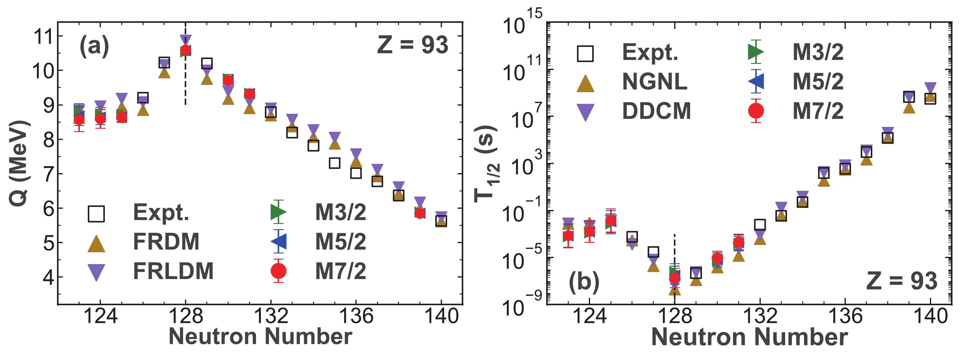
Figure 6. (color online) Similar to Fig. 2 but for the Neptunium isotopes.
For the Uranium isotopic chain, the α-decay energies and half-lives of the unknown nuclei
$ ^{213,220} {\rm{U}}$ are predicted using the Gaussian process with three kernel functions, as shown in Fig. 2. Moreover, the unknown α-decay energies of the$ ^{217} {\rm{U}}$ are predicted. It can be seen from Fig. 2 that both the predictive α-decay energies and half-lives are in good agreement with the results calculated with the traditional models. First, we would like to discuss the predictive results for the α-decay energies, which are shown in Fig. 2(a). The α-decay energies predicted for$ ^{213} {\rm{U}}$ and$ ^{220} {\rm{U}}$ are similar to those calculated using the traditional models. For$ ^{220} {\rm{U}}$ with N = 128, the predicted α-decay energies are the largest compared with the α-decay energies of the other Uranium isotopes shown in Fig. 2(a). Then, we focus on the known α-decay energies of nuclei with N = 128, e.g.,$ ^{217} {\rm{Ac}}$ in Fig. 3,$ ^{218} {\rm{Th}}$ in Fig. 4, and$ ^{219} {\rm{Pa}}$ in Fig. 5. All of these have the largest α-decay energies among their corresponding isotopes. This systematical behavior can be attributed to the shell effect [76, 77]. The parent nuclei with N = 128 are more likely to decay into the daughter nuclei with N = 126, which is a magic number. Thus, the largest α-decay energies are observed at N = 128 for the parent nuclei. Then, as shown in Fig. 2(b), for the predictive α-decay half-lives of$ ^{213} {\rm{U}}$ and$ ^{220} {\rm{U}}$ , they coincide with the theoretical results calculated using the NGNL and DDCM. In addition, for$ ^{220} {\rm{U}}$ , the predictive α-decay half-lives are the smallest in Fig. 2(b), which means it tends to spontaneously emit an α-particle to be stable. Apparently, both the predictive α-decay energies and half-lives show the shell effect. Thus, the Gaussian process can be used to characterize the α-decay properties even near the shell closure. Based on the above discussion, we can confirm that the predictive α-decay properties for the Uranium isotopes are as trustworthy as the calculated results obtained using the traditional models.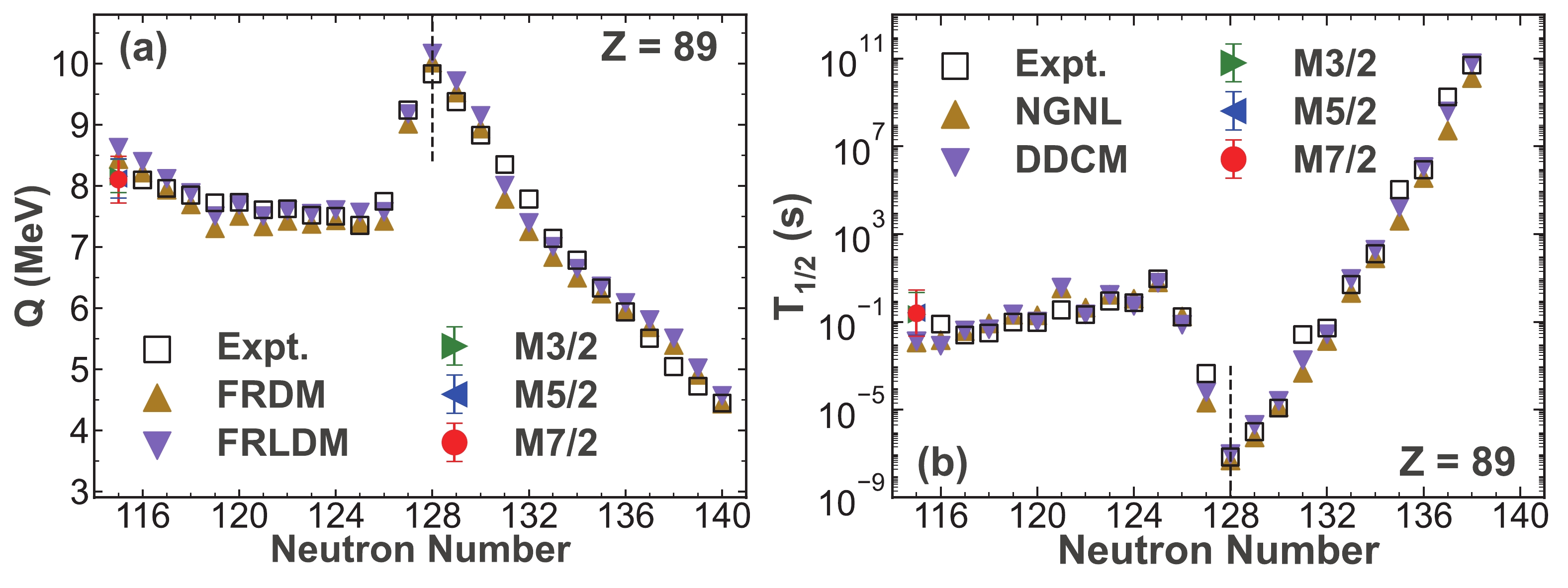
Figure 3. (color online) Similar to Fig. 2 but for the Actinium isotopes.
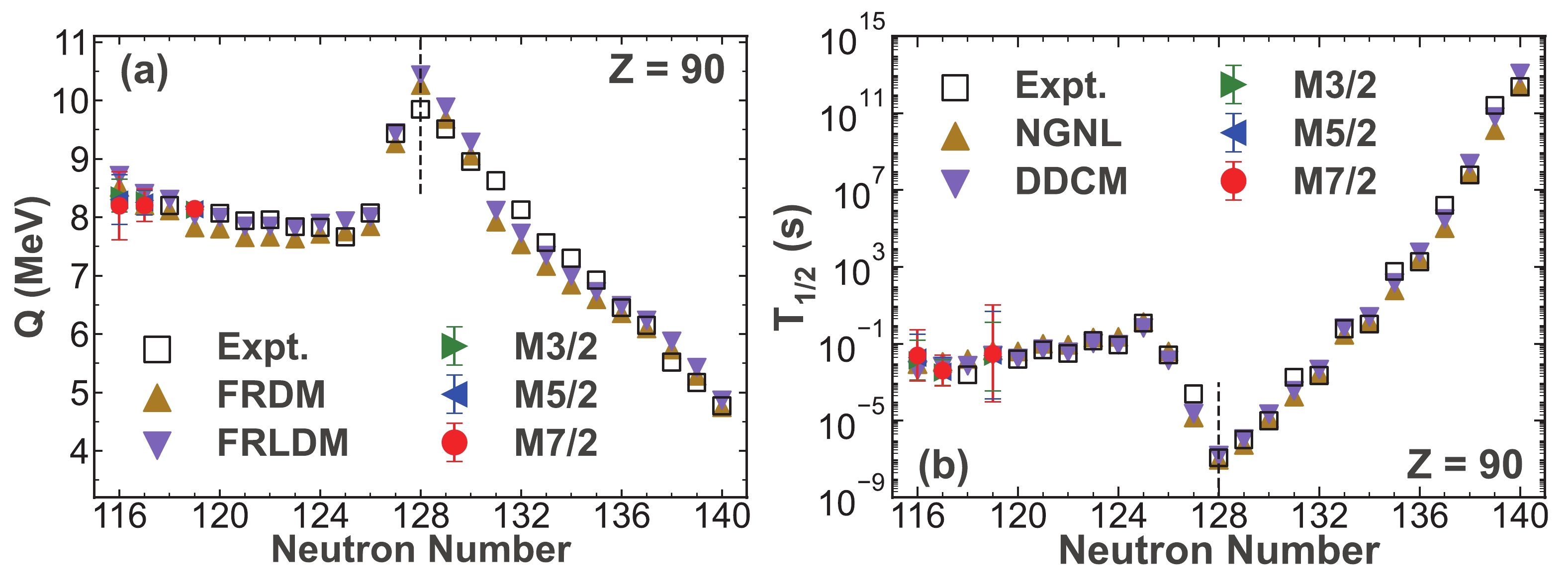
Figure 4. (color online) Similar to Fig. 2 but for the Thorium isotopes.
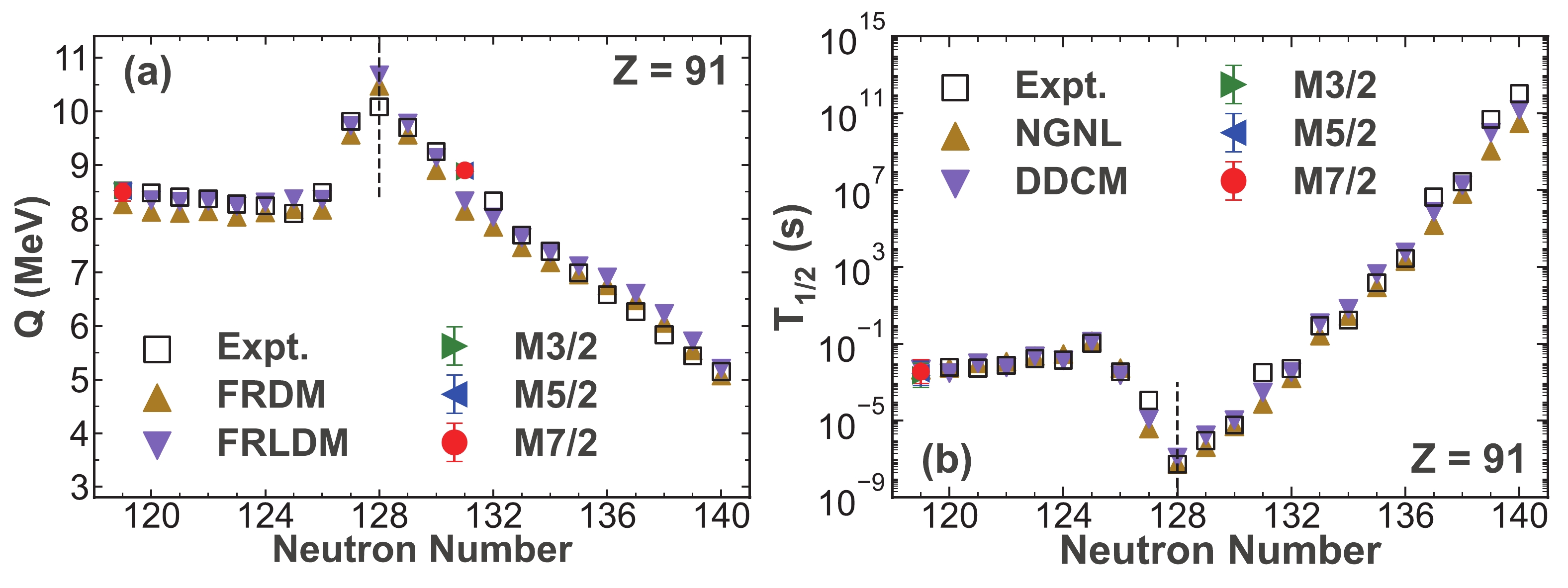
Figure 5. (color online) Similar to Fig. 2 but for the Protactinium isotopes.
Similarly, the α-decay properties of
$ ^{204} {\rm{Ac}}$ predicted using the Gaussian process for the Actinium isotopes are shown in Fig. 3. Regarding the Thorium isotopic chain, the α-decay properties of$ ^{206,207,209} {\rm{Th}}$ are forecast, which are shown in Fig. 4. Meanwhile, the α-decay energies and half-lives of$ ^{210} {\rm{Pa}}$ are predicted using the Gaussian process, as shown in Fig. 5, for the Protactinium isotopes. In addition, we calculate the unknown α-decay energies of$ ^{222} {\rm{Pa}}$ using the three kernel functions. The Neptunium isotopic chain is of great interest at present. In this work, we predict the α-decay properties of the unknown nuclei$ ^{216-218,221,224} {\rm{Np}}$ , and the results are shown in Fig. 6. Moreover, we predict the unknown α-decay energies of$ ^{232} {\rm{Np}}$ . It can be clearly observed that, in Fig. 3(a) - Fig. 6(a), the predictive α-decay energies are, respectively, very close to the calculated values extracted from the FRDM and FRLDM, and the predictive α-decay half-lives show good agreement with the results calculated using the NGNL and DDCM, respectively, in Fig. 3(b) - Fig. 6(b). Hence, the predictive α-decay properties obtained with the Gaussian process are consistent with the results calculated with the traditional models. Remarkably, the predictive α decay properties of$ ^{221} {\rm{Np}}$ shown in Fig. 6 with N = 128 also exhibit the shell effect similar to those of$ ^{220} {\rm{U}}$ , as shown in Fig. 2. Thus, the Gaussian process can be considered to be a trustworthy model for predicting the α-decay properties and can be used to characterize the α-decay properties even near the shell closure. Furthermore, because of the similar predictive results of the α-decay energies and half-lives obtained using the three kernel functions, it can be concluded that the systematic error of the Gaussian process is small.Finally, we use the Gaussian process to predict the α-decay properties of some unknown neutron-deficient Plutonium isotopes, as only
$ ^{228-234} {\rm{Pu}}$ have been synthesized until now and there remain gaps in the experimental observations for the Plutonium isotopic chain. We predict the α-decay energies of$ ^{217-227} {\rm{Pu}}$ , with the corresponding results listed in Table 3, and the α-decay half-lives of$ ^{227} {\rm{Pu}}$ , with the corresponding results presented in Table 4, using the Gaussian process. Only the α-decay half-life of$ ^{227} {\rm{Pu}}$ is predicted because the angular momentums of the other nuclei are uncertain. In Table. 3, the first column shows the parent nuclei for α decay. The second, third, and fourth columns show the predictive α-decay energies obtained with the Matérn 3/2, Matérn 5/2, and Matérn 7/2 kernel functions, respectively. The last two columns present the calculated α-decay energies extracted from the FRDM and FRLDM, respectively. In Table 4, the first column lists the parent nucleus for α decay. The second, third, and fourth columns show the predictive α-decay half-lives obtained with the Matérn 3/2, Matérn 5/2, and Matérn 7/2 kernel functions, respectively. The last two columns, respectively, present the α-decay half-lives calculated using the NGNL and DDCM. The predictive α-decay properties for the Plutonium isotopes versus the neutron number are plotted in Fig. 7. It can be observed that the α-decay energy of$ ^{222} {\rm{Pu}}$ with N = 128 is the largest, which also shows the effect of the shell closure. This peak can be seen clearly in Fig. 7(a) at N = 128. Furthermore, in Fig. 7(a), most of the predictive α-decay energies are consistent with the calculated results derived from the FRDM and FRLDM except for those predicted for$ ^{217-219} {\rm{Pu}}$ . Based on the predictive results for$ ^{217-219} {\rm{Pu}}$ in Fig. 7(a), it can be seen that with increasing extrapolation distance, the systematic error of the Gaussian process is large. For$ ^{217-219} {\rm{Pu}}$ , the predictive α-decay energies obtained with the Matérn 3/2 kernel function are in agreement with those obtained with the FRDM and FRLDM, while the α-decay energies obtained with the Matérn 5/2 and Matérn 7/2 kernel functions show differences from the results calculated with the traditional models, respectively. These differences must be confirmed in future experiments. In Fig. 7(b), the predictive α-decay half-lives of$ ^{227} {\rm{Pu}}$ show good agreement with the results calculated with the NGNL and DDCM. Previous studies have reported general difficulties with respect to extrapolation within the framework of the Gaussian process [61-63]. A similar problem may also exist in this work, and we expect that this problem can be further improved upon. We hope that our theoretical predictions will be helpful for the synthesis experiments of neutron-deficient actinide nuclei in the future.Nucl. $ Q_{M_{3/2}}/{\rm{MeV}} $ 

$Q_{M_{5/2} }/{\rm{MeV} }$ 

$ Q_{M_{7/2}}/{\rm{MeV}} $ 

$ Q_{22a} /{\rm{MeV}}$ 

$ Q_{22b}/{\rm{MeV}}$ 

$ ^{217} {\rm{Pu}}$ 

8.997 8.594 8.204 8.925 9.165 $ ^{218} {\rm{Pu}}$ 

8.988 8.697 8.442 8.975 9.205 $ ^{219} {\rm{Pu}}$ 

9.142 8.977 8.843 9.185 9.435 $ ^{220} {\rm{Pu}}$ 

9.663 9.665 9.634 9.165 9.395 $ ^{221} {\rm{Pu}}$ 

10.384 10.515 10.545 10.135 10.365 $ ^{222} {\rm{Pu}}$ 

10.658 10.816 10.844 10.865 11.105 $ ^{223} {\rm{Pu}}$ 

10.422 10.481 10.447 10.055 10.295 $ ^{224} {\rm{Pu}}$ 

9.980 9.942 9.853 9.565 9.805 $ ^{225} {\rm{Pu}}$ 

9.474 9.404 9.311 9.285 9.505 $ ^{226} {\rm{Pu}}$ 

8.901 8.815 8.730 9.035 9.255 $ ^{227} {\rm{Pu}}$ 

8.350 8.284 8.233 8.695 8.925 Table 3. Predictions on the α-decay energies for the unknown Pu isotopes. The first column shows the parent nuclei for α-decay. The second, third, and fourth columns show the predictive α-decay energies obtained with the Matérn 3/2, Matérn 5/2, and Matérn 7/2 kernel functions, respectively. The last two columns present the calculated α-decay energies extracted from the FRDM and FRLDM, which are denoted as 22a and 22b, respectively.
Nucl. $ T_{1/2}^{M_{3/2}} /{\rm{s}}$ 

$ T_{1/2}^{M_{5/2}}/{\rm{s}} $ 

$ T_{1/2}^{M_{7/2}}/{\rm{s}} $ 

$ T_{1/2}^{\rm NGNL} /{\rm{s}}$ 

$ T_{1/2}^{\rm DDCM}/{\rm{s}} $ 

$ ^{227} {\rm{Pu}}$ 

1.15 $ \times 10^{-1} $ 

2.49 $ \times 10^{-1} $ 

4.05 $ \times 10^{-1} $ 

4.37 $ \times 10^{-2} $ 

1.08 $ \times 10^{-1} $ 

Table 4. Predictions on the α-decay half-lives for the unknown Pu isotope. The first column shows the parent nucleus for α-decay. The second, third, and fourth columns present the predictive α-decay half-lives obtained with the Matérn 3/2, Matérn 5/2, and Matérn 7/2 kernel functions, respectively. The last two columns show the calculated α-decay half-lives obtained with the NGNL and DDCM, respectively.
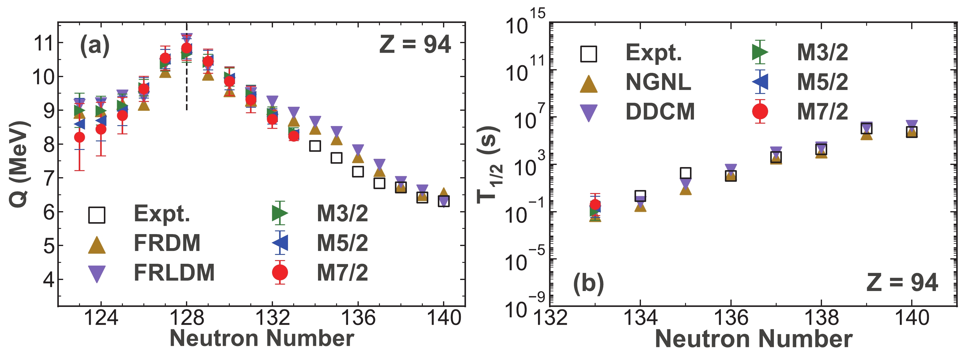
Figure 7. (color online) Similar to Fig. 2 but for the Plutonium isotopes.
-
In summary, a new model is used to predict the α-decay energies and half-lives of some unknown neutron-deficient nuclei with 89
$\leqslant $ Z$\leqslant $ 94 within the framework based on a machine learning algorithm called the Gaussian process. Three kernel functions, namely the Matérn 3/2, Matérn 5/2, and Matérn 7/2 kernel functions, are used to obtain the systematic error of the Gaussian process in this work. First, the α-decay properties of the new actinide nucleus$ ^{214} {\rm{U}}$ are calculated. The deviations between the experimental result and the α-decay energies calculated with the Matérn 3/2, Matérn 5/2, and Matérn 7/2 kernel functions are 0.017 MeV, 0.044 MeV, and 0.063 MeV, respectively. The predictive α-decay half-lives show good agreement with the experimental result with a factor of 1.240, 1.289, and 1.376, respectively. It can be seen that the calculated results of both the α-decay energies and half-lives agree well with the latest experimental results. This shows the reliability of the Gaussian process for predicting the α-decay properties. Then, we further use the Gaussian process to calculate the α-decay properties of some unknown neutron-deficient nuclei with 89$\leqslant $ Z$\leqslant $ 93. The predictive α-decay energies show good agreement with the results extracted from the FRDM and FRLDM. Moreover, the α-decay half-lives are in good accordance with the theoretical results calculated with the NGNL and DDCM. These comparative results show that the Gaussian process is a trustworthy model for predicting the α-decay properties. Noticeably, the predictive α-decay properties of$ ^{220} {\rm{U}}$ and$ ^{221} {\rm{Np}}$ show the systematical behaviors at N = 128, which indicates that the Gaussian process can be applied to characterize the α-decay properties even near the shell closure. Finally, the α-decay energies of the unknown$ ^{217-227} {\rm{Pu}}$ and the α-decay half-lives of the unknown$ ^{227} {\rm{Pu}}$ are obtained, for the Plutonium isotopes, where few isotopes have been synthesized in experiments to date. Furthermore, the calculated results show that the systematic error of the Gaussian process is small. We believe that our work can serve as a useful reference for further studies on neutron-deficient actinide nuclei. Our work provides a new method for research on α decay based on machine learning, and we hope that more machine learning approaches (e.g., learning machine [78]) can be generalized to study α decay in the future. -
The authors would like to thank Prof. Jin Lei from Tongji University and Prof. Chen Ji from Central China Normal University for their helpful discussions. We thank Prof. Hong Zhao from Xiamen University for discussions on machine learning during his visit to Tongji University. We would also like to thank the anonymous referees for their constructive comments and suggestions.
Theoretical predictions on α-decay properties of some unknown neutron-deficient actinide nuclei using machine learning
- Received Date: 2021-08-23
- Available Online: 2022-02-15
Abstract: Neutron-deficient actinide nuclei provide a valuable window to probe heavy nuclear systems with large proton-neutron ratios. In recent years, several new neutron-deficient Uranium and Neptunium isotopes have been observed using α-decay spectroscopy [Z. Y. Zhang et al., Phys. Rev. Lett. 122, 192503 (2019); L. Ma et al., Phys. Rev. Lett. 125, 032502 (2020); Z. Y. Zhang et al., Phys. Rev. Lett. 126, 152502 (2021)]. In spite of these achievements, some neutron-deficient key nuclei in this mass region are still unknown in experiments. Machine learning algorithms have been applied successfully in different branches of modern physics. It is interesting to explore their applicability in α-decay studies. In this work, we propose a new model to predict the α-decay energies and half-lives within the framework based on a machine learning algorithm called the Gaussian process. We first calculate the α-decay properties of the new actinide nucleus


 DownLoad: