


 Abstract
 HTML
HTML Reference
 Related
 PDF
PDF


-
There are still many classical problems in modern theoretical physics that cannot be properly interpreted by the Standard Model (SM), such as the hierarchy problem [1-6], cosmological problem [7-14], and the nature of dark matter and dark energy [15-18]. Since the famous Arkani-Hamed, Dimopoulos and Dvali (ADD) [1] and Randall-Sundrum (RS) brane-world models [2, 19] were presented, the extra dimension and brane-world theories have gradually attracted more attention because they can provide new mechanisms to solve these classical problems. Unlike early models in which a brane is a geometric hypersurface embedded in a higher dimensional spacetime, a more realistic brane should have thickness and an inner structure. Such thick branes can be generated by bulk matter fields (mostly scalar fields) [20-40], or can be realized in pure gravities [41-43] (see Refs. [29, 44] for detailed introduction of thick brane models).
In the braneworld scenario, an important and interesting issue is to investigate the mechanism of localizing the various fields' Kaluza-Klein (KK) modes on branes. These KK modes contain the information of extra dimensions. Especially, the zero modes of matter fields on the brane stand for the four-dimensional massless particles, and they can rebuild the SM on branes at low energy. A lot of research about the localization of various fields on branes have been conducted [45-68]. Besides, the Elko spinor, which is named from the eigenspinor of the charge conjugation operator, has attracted interest since it was introduced by Ahluwalia and Grumiller in
$ 2005 $ [69, 70]. It is a new spin-$ 1/2 $ quantum field that satisfies the Klein-Gordon (KG) equation instead of the Dirac one, and only interacts with itself, Higg fields, and gravity [69-76]. As a candidate of dark matter, it was widely investigated in particle physics [69-72], cosmology [77-86], and mathematical physics [87-93].In Refs. [94-96], the localization of the zero mode of a five-dimensional Elko spinor on various Minkowski branes was considered. A coupling mechanism should be introduced in order to localize the Elko zero mode on a brane. The first choice is the Yukawa-type coupling
$ -\eta F(\phi $ or$ R)\mathop \lambda\limits^\neg\lambda $ between the five-dimensional Elko spinor$ \lambda $ and the background scalar field$ \phi $ [94, 95] or the Ricci scalar$ R $ [96]. Here$ F $ is a function of the background scalar field or the Ricci scalar and$ \eta $ is the coupling constant. Recently, another localization mechanism, i.e., the non-minimal coupling$ f(\phi)\mathfrak{L}_{\rm Elko} $ between the Elko spinor and the background scalar field, was investigated in Ref. [97]. Here$ \mathfrak{L}_{\rm Elko} $ is the Lagrangian of the Elko spinor and$ f(\phi) $ is a function of the background scalar field. It was shown that by introducing an auxiliary function$ K(z) $ in the conformal coordinate$ z $ , the general expression of the Elko zero mode$ \alpha_0 $ and the scalar function$ f(\phi) $ could be obtained. Different forms of$ K(z) $ will lead to different solutions of the zero mode and the scalar function. Thus, a non-minimal coupling can also provide the possibility of localizing the Elko zero mode. However, all current localizations of the five-dimensional Elko spinor are based on Minkowski branes.It is well known that the properties of de Sitter (dS) and Anti-de Sitter (AdS) thick branes are very different from those of Minkowski branes, so compared to the localization on Minkowski branes, the results of the localization on dS/AdS thick branes should be very different. Thus, the localization of a five-dimensional Elko spinor on dS/AdS thick branes is an interesting topic. In this paper, we analyze two types of localization mechanism to confine the five-dimensional Elko zero mode on dS/AdS branes and investigate their differences and similarities. It will be shown that both types can achieve the localization of the five-dimensional Elko spinor on dS/AdS thick branes, and the coupling functions
$ F(\phi) $ and$ f(\phi) $ play a similar role. We believe that investigating the differences and similarities between them will be helpful to further explore the new localization mechanism and expand the possibility of localizing fields on branes.This paper is organized as follows. We first review the Yukawa-type and non-minimal couplings in Sec. II. The localization of the zero mode of a five-dimensional Elko spinor on the dS/AdS thick branes is investigated by considering two different coupling mechanisms in Sec. III. Then in Sec. IV, we consider the localization of the Elko zero mode on another AdS thick brane. Finally, a brief conclusion is given in Sec. V.
-
In this section, we review two localization mechanisms of the five-dimensional Elko spinor on thick branes, namely the Yukawa-like coupling and the non-minimal coupling between the Elko spinor and the background scalar field that generates the thick brane.
The line-element is generally assumed as
$ {\rm d}s^{2} = \text{e}^{2A(y)}\hat{g}_{\mu\nu}{\rm d}x^{\mu}{\rm d}x^{\nu}+{\rm d}y^{2}, $

(1) where the warp factor
$ \text{e}^{2A(y)} $ is a function of the extra dimension coordinate$ y $ . By performing the conformal coordinate transformation$ {\rm d}z = \text{e}^{-A(y)}{\rm d}y, $

(2) the metric in Eq. (1) is transformed as
$ {\rm d}s^{2} = \text{e}^{2A}(\hat{g}_{\mu\nu}{\rm d}x^{\mu}{\rm d}x^{\nu}+{\rm d}z^{2}), $

(3) which is more convenient for discussing the localization of gravity and various matter fields.
-
First, we start with the action of a five-dimensional massless Elko spinor
$ \begin{aligned}[b] S =& \int {\rm d}^5x\sqrt{-g}\mathfrak{L}_{\rm Elko}, \\ \mathfrak{L}_{\text{Elko}} =& -\frac{1}{4}g^{MN}\left(\mathfrak{D}_{M}\mathop \lambda\limits^\neg\mathfrak{D}_{N}\lambda+\mathfrak{D}_{N}\mathop \lambda\limits^\neg\mathfrak{D}_{M}\lambda\right)\\&-\eta F(\phi)\mathop \lambda\limits^\neg\lambda,\; \end{aligned} $

(4) where the last term is the Yukawa-like coupling,
$ F(\phi) $ is the coupling function of the background scalar field$ \phi $ , and$ \eta $ is the coupling constant. In this paper,$ M,N,\cdots = 0,1,2,3,5 $ and$ \mu,\nu,\cdots = 0,1,2,3 $ denote the five-dimensional and four-dimensional spacetime indices, respectively. The covariant derivatives are$ \mathfrak{D}_{M}\lambda = (\partial_{M}+\Omega_{M})\lambda,\quad \mathfrak{D}_{M}\mathop \lambda\limits^\neg = \partial_{M}\mathop \lambda\limits^\neg-\mathop \lambda\limits^\neg\Omega_{M}, $

(5) where the spin connection
$ \Omega_{M} $ is defined as$ \begin{aligned}[b]\Omega_{M} =& -\frac{\rm i}{2}\left(e_{\bar{A}P}e_{\bar{B}}^{\; \; N} \Gamma^{P}_{MN} -e_{\bar{B}}^{\; \; N}\partial_{M}e_{\bar{A}N}\right) S^{\bar{A}\bar{B}}, \\ S^{\bar{A}\bar{B}} =& \frac{\rm i}{4}\Big[\gamma^{\bar{A}},\gamma^{\bar{B}}\Big]. \end{aligned} $

(6) Here
$ e^{\bar{A}}_{\; M} $ is the vierbein and satisfies the orthonormality relation$ g_{MN} = e^{\bar{A}}_{\; M}e^{\bar{B}}_{\; N}\eta_{\bar{A}\bar{B}} $ .$ \bar{A},\bar{B}\cdots = 0,1,2,3,5 $ denote the five-dimensional local Lorentz indices. Thus, the non-vanishing components of the spin connection$ \Omega_{M} $ are$ \Omega_{\mu} = \frac{1}{2}\partial_{z}A\gamma_{\mu}\gamma_{5} + \hat{\Omega}_{\mu} . $

(7) Here
$ \gamma_{\mu} $ and$ \gamma_{5} $ are the four-dimensional gamma matrixes on the brane, and they satisfy$ \{\gamma^{\mu},\gamma^{\nu}\} = 2\hat{g}^{\mu\nu} $ .Then, the equation of motion for the Elko spinor coupled with the scalar field is read as
$ \frac{1}{\sqrt{-g}}\mathfrak{D}_{M}(\sqrt{-g}g^{MN}\mathfrak{D}_{N}\lambda)-2\eta F(\phi)\lambda = 0. $

(8) By considering the metric in Eq. (3) and using the non-vanishing components of the spin connection in Eq. (7), the above equation can be rewritten as
$ \begin{aligned}[b]& \frac{1}{\sqrt{-\hat{g}}}\hat{\mathfrak{D}}_{\mu}\Big(\sqrt{-\hat{g}}\hat{g}^{\mu\nu}\hat{\mathfrak{D}}_{\nu}\lambda\Big) +\bigg[-\frac{1}{4}{A'}^{2}\hat{g}^{\mu\nu}\gamma_{\mu}\gamma_{\nu}\lambda\\ +&\frac{1}{2}A' \left( \frac{1}{\sqrt{-\hat{g}}} \hat{\mathfrak{D}}_{\mu} \Big( {\sqrt{-\hat{g}}} \hat{g}^{\mu\nu}\gamma_{\nu}\gamma_{5}\lambda\Big) +\hat{g}^{\mu\nu}\gamma_{\mu}\gamma_{5}\hat{\mathfrak{D}}_{\nu}\lambda\right) \\ +&\text{e}^{-3A}\partial_{z}\big(\text{e}^{3A}\partial_{z}\lambda\big)\bigg]-2\eta \text{e}^{2A}F(\phi)\lambda = 0. \end{aligned} $

(9) Here
$ \hat{g}_{\mu\nu} $ is the induced metric on the brane, and$ \hat{\mathfrak{D}}_{\mu}\lambda = (\partial_{\mu}+\hat{\Omega}_{\mu})\lambda $ with$ \hat{\Omega}_{\mu} $ denoting the spin connection constructed by the induced metric$ \hat{g}_{\mu\nu} $ . From$ \hat{\mathfrak{D}}_{\mu}\hat{e}^{a}_{\; \nu} = 0 $ , we can obtain$ \hat{\mathfrak{D}}_{\mu}\hat{g}^{\lambda\rho} = \hat{\mathfrak{D}}_{\mu}(\hat{e}_{a}^{\; \lambda}\hat{e}^{a\rho}) = 0 $ . Thus, the above equation can be simplified as$ \begin{aligned}[b]&\frac{1}{\sqrt{-\hat{g}}}\hat{\mathfrak{D}}_{\mu}\Big(\sqrt{-\hat{g}}\hat{g}^{\mu\nu}\hat{\mathfrak{D}}_{\nu}\lambda\Big) - A'\gamma^{5}\gamma^{\mu} \hat{\mathfrak{D}}_{\mu}\lambda - {A'}^{2}\lambda \\+&\text{e}^{-3A}\partial_{z}\big(\text{e}^{3A}\partial_{z}\lambda\big)-2\eta\text{e}^{2A} F(\phi)\lambda = 0.\end{aligned} $

(10) Next, we introduce the following KK decomposition
$ \begin{aligned}[b] \lambda_{\pm} =& \text{e}^{-3A/2}\sum_{n}\left(\alpha_{n}(z)\varsigma^{(n)}_{\pm}(x)+\alpha_{n}(z)\tau^{(n)}_{\pm}(x)\right)\\ =& \text{e}^{-3A/2}\sum_{n}\alpha_{n}(z)\hat{\lambda}_{\pm}^{n}(x). \end{aligned} $

(11) For simplicity, we omit the
$ \pm $ subscript for the$ \alpha_n $ functions in the following. Note that$ \varsigma^{n}_{\pm}(x) $ and$ \tau^{(n)}_{\pm}(x) $ are linear independent four-dimensional Elko spinors, and they satisfy$ \gamma^{\mu}\hat{\mathfrak{D}}_{\mu}\varsigma_{\pm}(x) = \mp\text{i}\varsigma_{\mp}(x),\quad \gamma^{\mu}\hat{\mathfrak{D}}_{\mu}\tau_{\pm}(x) = \pm\text{i}\tau_{\mp}(x), $

(12) $ \gamma^5\varsigma_{\pm}(x) = \pm\tau_{\mp}(x),\; \; \; \; \; \; \gamma^5\tau_{\pm}(x) = \mp\varsigma_{\mp}(x). $

(13) The four-dimensional Elko spinor
$ \hat{\lambda}^{n} $ should satisfy the K-G equation:$ \frac{1}{\sqrt{-\hat{g}}}\hat{\mathfrak{D}}_{\mu}(\sqrt{-\hat{g}}\hat{g}^{\mu\nu}\hat{\mathfrak{D}}_{\nu}\hat\lambda^n) = m^2_n\hat\lambda^n $

(14) with
$ m_n $ the mass of the Elko spinor on the brane. Thus, we obtain the following equations of motion for the Elko KK modes$ \alpha_{n} $ :$ \alpha_{n}''-\Bigg(\frac{3}{2}A''+\frac{13}{4}(A')^{2}+2\eta\text{e}^{2A}F(\phi)-m_{n}^2+\text{i}m_{n}A'\Bigg)\alpha_{n} = 0. $

(15) For the purpose of deriving the action of the four-dimensional massless and massive Elko spinors from the action of a five-dimensional massless Elko spinor with Yukawa-like coupling as follows:
$ \begin{aligned}[b]S_{\text{Elko}} =& \int {\rm d}^5x\sqrt{-g}\,\bigg[-\frac{1}{4}g^{MN}(\mathfrak{D}_M\mathop \lambda\limits^\neg\mathfrak{D}_{N}\lambda\\&+\mathfrak{D}_N\mathop \lambda\limits^\neg\mathfrak{D}_{M}\lambda)-\eta F(\phi)\mathop \lambda\limits^\neg\lambda\bigg]\\ =& -\frac{1}{2}\sum_{n}\int {\rm d}^4x\bigg[\frac{1}{2}\hat{g}^{\mu\nu}(\hat{\mathfrak{D}_\mu}\hat{\mathop \lambda\limits^\neg}^{n}\hat{\mathfrak{D}_{\nu}}\hat{\lambda}^{n}\\&+\hat{\mathfrak{D}_\nu}\hat{\mathop \lambda\limits^\neg}^{n}\hat{\mathfrak{D}_{\mu}}\hat{\lambda}^{n})+m_{n}^2\hat{{\mathop \lambda\limits^\neg}}^{n}\hat{\lambda}^{n}\bigg], \end{aligned} $

(16) we should introduce the following orthonormality condition for
$ \alpha_{n} $ :$ \int \alpha^{*}_{n}\alpha_{m}{\rm d}z = \delta_{nm}. $

(17) For the Elko zero mode (
$ m_0 = 0 $ ), Eq. (15) becomes$ \big[-\partial_{z}^{2}+V^{Y}_{0}(z)\big]\alpha_{0}(z) = 0, $

(18) where
$ V^{Y}_{0}(z) = \frac{3}{2}A''+\frac{13}{4}{A'}^{2}+2\eta \text{e}^{2A}F(\phi). $

(19) In this case, the orthonormality condition is given by
$\int \alpha^*_0\alpha_0{\rm d}z = 1. $

(20) As we showed in a previous study of ours [94], there exist many similarities between the Elko field and the scalar field. For a five-dimensional free massless scalar field, the Schrödinger-like equation for the scalar zero mode
$ h_0 $ [49, 94] can be expressed as$ \begin{aligned}[b] \left[-\partial_{z}^{2}+V_{\Phi}\right]h_0 =& \left[-\partial_{z}^{2}+\frac{3}{2}A''+\frac{9}{4}{A'}^{2}\right]h_0\\ =& \left[\partial_{z}+\frac{3}{2}A'\right]\left[-\partial_{z}+\frac{3}{2}A'\right]h_{0}\\ =& 0. \end{aligned} $

(21) The solution is given by
$ h_{0}(z)\varpropto\text{e}^{\frac{3}{2}A(z)} $ and it satisfies the orthonormality relation for any brane embedded in a five-dimensional Anti-de Sitter (AdS) spacetime. However, the effective potential$ V_0 $ for the five-dimensional free massless Elko spinor is [94]$ V_0(z) = \frac{3}{2}A''+\frac{13}{4}A'^2 = \frac{3}{2}A''+\frac{9}{4}A'^2+A'^2. $

(22) The additional term
$ A'^2 $ prevents the localization of the zero mode.When the Yukawa-like coupling is introduced, the coefficient numbers of
$ A'' $ and$ A'^2 $ can be regulated:$ \frac{3}{2}A''+\frac{13}{4}{A'}^{2}+2\eta \text{e}^{2A}F(\phi) = (p A')'+(p A')^2, $

(23) where
$ p $ is a real constant. From Eq. (23), the form of$ F(\phi) $ can be obtained$ F(\phi) = -\frac{1}{2\eta}\text{e}^{-2A}\left[\left(p-\frac{3}{2}\right)A''+\left(p^2-\frac{13}{4}\right)A'^2\right].\; \; \; \; $

(24) Then, Eq. (18) can be rewritten as
$ \begin{aligned}[b][-\partial_{z}^{2}+V^{Y}_{0}]\alpha_{0} =& [-\partial_{z}^{2}+p A''+p^2A'^2]\alpha_{0}\\ =& \left[\partial_{z}+p A'\right]\left[-\partial_{z}+p A'\right]\alpha_{0} \\ =& 0,\end{aligned}$

(25) and the Elko zero mode becomes
$ \alpha_0(z)\varpropto\text{e}^{p A(z)}. $

(26) -
On the other hand, for the non-minimal coupling, the action could be written as
$ \begin{aligned}[b] S =& \int {\rm d}^5x\sqrt{-g}f(\phi)\mathfrak{L}_{\text{Elko}}, \\ \mathfrak{L}_{\text{Elko}} =& -\frac{1}{4}g^{MN}\left(\mathfrak{D}_{M}\mathop \lambda\limits^\neg\mathfrak{D}_{N}\lambda+\mathfrak{D}_{N}\mathop \lambda\limits^\neg\mathfrak{D}_{M}\lambda\right). \end{aligned} $

(27) Here
$ f(\phi) $ is a function of the background scalar field$ \phi $ , which is a function of the extra dimension coordinate$ z $ (or$ y $ ). From the action in Eq. (27), the following equation of motion can be derived:$ \frac{1}{\sqrt{-g}f(\phi)}\mathfrak{D}_{M}(\sqrt{-g}f(\phi)g^{MN}\mathfrak{D}_{N}\lambda) = 0. $

(28) By considering the metric in Eq. (3) and using the non-vanishing components of the spin connection in Eq. (7), we can rewrite Eq. (28) as follows:
$ \begin{aligned}[b] &\frac{1}{\sqrt{-\hat{g}}}\hat{\mathfrak{D}}_{\mu}\Big(\sqrt{-\hat{g}}\hat{g}^{\mu\nu}\hat{\mathfrak{D}}_{\nu}\lambda\Big) +\bigg[-\frac{1}{4}{A'}^{2}\hat{g}^{\mu\nu}\gamma_{\mu}\gamma_{\nu}\lambda\\ &+\frac{1}{2}A' \left( \frac{1}{\sqrt{-\hat{g}}} \hat{\mathfrak{D}}_{\mu} ( {\sqrt{-\hat{g}}} \hat{g}^{\mu\nu}\gamma_{\nu}\gamma_{5}\lambda) +\hat{g}^{\mu\nu}\gamma_{\mu}\gamma_{5}\hat{\mathfrak{D}}_{\nu}\lambda\right) \\ &+\text{e}^{-3A}f^{-1}(\phi)\partial_{z}(\text{e}^{3A}f(\phi)\partial_{z}\lambda)\bigg]\\ = &\frac{1}{\sqrt{-\hat{g}}}\hat{\mathfrak{D}}_{\mu}\Big(\sqrt{-\hat{g}}\hat{g}^{\mu\nu}\hat{\mathfrak{D}}_{\nu}\lambda\Big) - A'\gamma^{5}\gamma^{\mu} \hat{\mathfrak{D}}_{\mu}\lambda - {A'}^{2}\lambda\\ &+\text{e}^{-3A}f^{-1}(\phi)\partial_{z}(\text{e}^{3A}f(\phi)\partial_{z}\lambda) = 0. \end{aligned} $

(29) In this case, we introduce the following KK decomposition:
$ \begin{aligned}[b] \lambda_{\pm} =& \text{e}^{-3A/2}f(\phi)^{-1/2}\sum_{n}\left(\alpha_{n}(z)\varsigma^{(n)}_{\pm}(x)+\alpha_{n}(z)\tau^{(n)}_{\pm}(x)\right)\\ =& \text{e}^{-3A/2}f(\phi)^{-1/2} \sum_{n}\alpha_{n}(z)\hat{\lambda}_{\pm}^{n}(x). \end{aligned} $

(30) By noticing the linear independence of the
$ \varsigma^{(n)}_{+} $ and$ \tau^{(n)}_{+} $ ($ \varsigma^{(n)}_{-} $ and$ \tau^{(n)}_{-} $ ) and the K-G equation of the four-dimenional Elko spinor, the equation of motion of the KK mode$ \alpha_{n} $ can be derived:$ \begin{aligned}[b]& \alpha_{n}''-\Bigg(-\frac{1}{4}f^{-2}(\phi)f'^{2}(\phi)+\frac{3}{2}A'f^{-1}(\phi)f'(\phi)+\frac{1}{2}f^{-1}(\phi)f''(\phi)\\ +&\frac{3}{2}A''+\frac{13}{4}(A')^{2}-m_{n}^2+\text{i}m_{n}A'\Bigg)\alpha_{n} = 0. \end{aligned} $

(31) For the non-minimal coupling case, by introducing the same orthonormality conditions as in Eq. (17), we can derive the action of the four-dimensional massless and massive Elko spinors from the action in Eq. (27):
$ \begin{aligned}[b] S_{\text{Elko}} =& -\frac{1}{4}\int {\rm d}^5x\sqrt{-g}f(\phi)g^{MN}(\mathfrak{D}_M\mathop \lambda\limits^\neg\mathfrak{D}_{N}\lambda+\mathfrak{D}_N\mathop \lambda\limits^\neg\mathfrak{D}_{M}\lambda)\\ =& -\frac{1}{2}\sum_{n}\int {\rm d}^4x\bigg[\frac{1}{2}\hat{g}^{\mu\nu}(\hat{\mathfrak{D}_\mu}\hat{\mathop \lambda\limits^\neg}^{n}\hat{\mathfrak{D}_{\nu}}\hat{\lambda}^{n}\\&+\hat{\mathfrak{D}_\nu}\hat{\mathop \lambda\limits^\neg}^{n}\hat{\mathfrak{D}_{\mu}}\hat{\lambda}^{n})+m_{n}^2\hat{{\mathop \lambda\limits^\neg}}^{n}\hat{\lambda}^{n}\bigg].\end{aligned} $

(32) For the Elko zero mode with
$ m_n = 0 $ , Eq. (31) is simplified as$ \left[-\partial_{z}^{2}+V^{N}_{0}(z)\right]\alpha_{0}(z) = 0, $

(33) where the effective potential
$ V^{N}_{0} $ is given by$ \begin{aligned}[b]V^{N}_{0}(z) =& -\frac{1}{4}f^{-2}(\phi)f'^{2}(\phi)+\frac{3}{2}A'f^{-1}(\phi)f'(\phi)\\&+\frac{1}{2}f^{-1}(\phi)f''(\phi)+\frac{3}{2}A''+\frac{13}{4}A'^2, \end{aligned} $

(34) and the Elko zero mode
$ \alpha_{0}(z) $ satisfies the orthonormality condition in Eq. (20). By introducing three new functions, namely$ B(z) $ ,$ C(z) $ , and$ D(z) $ , satisfying$ B(z) = \frac{f'(\phi)}{f(\phi)} = -3A'+\frac{A'^2}{C}-C-\frac{C'}{C}, $

(35) $ \partial_zD(z) = \frac{3}{2}A'+\frac{1}{2}B+C, $

(36) the effective potential in Eq. (34) becomes
$ V^{N}_0(z) = \frac{1}{4}B^2+\frac{3}{2}A'B+\frac{1}{2}B'+\frac{3}{2}A''+\frac{13}{4}A'^2\\ = D''+D'^2, $

(37) and Eq. (33) can be reduced as follows:
$ \begin{aligned}[b] [-\partial_{z}^{2}+V^N_{0}]\alpha_{0} =& [-\partial_{z}^{2}+D''+D'^2]\alpha_{0}\\ =& \left[\partial_{z}+D'\right]\left[-\partial_{z}+D'\right]\alpha_{0} \\ =& 0. \end{aligned} $

(38) In addition, it will be convenient to define a new function
$ K(z) $ :$ K(z)\equiv\frac{C'}{C}-C . $

(39) Note that the form of
$ K(z) $ is arbitrary, and the forms of$ C(z) $ and$ B(z) $ are determined by the warp factor and any given$ K(z) $ . Now it is easy to obtain the zero mode$ \alpha_0 $ :$ \begin{aligned}[b] \alpha_{0}(z)\varpropto \text{e}^{D(z)} & = {\exp} \left[\frac{1}{2}\int^{z}_{0}\left(\frac{A'^2}{C}-\frac{C'}{C}+ C \right){\rm d}\bar{z}\right]\\ & = {\exp}\left[\frac{1}{2}\int^{z}_{0}\left(\frac{A'^2}{C}-K\right){\rm d}\bar{z}\right]\\ & = {\exp}\left[\frac{1}{2}\int^{z}_{0}\frac{A'^2}{C}{\rm d}\bar{z}\right]{\exp}\left[-\frac{1}{2}\int^{z}_{0}K{\rm d}\bar{z}\right], \end{aligned} $

(40) and the form of
$ f(\phi) $ :$ \begin{aligned}[b] f(\phi(z)) =& \text{e}^{\int^{z}_{0} B(\bar{z}) {\rm d}\bar{z}} = {\exp}\left[\int^{z}_{0}\left( -3A'+\frac{A'^2}{C}- C-\frac{C'}{C} \right) {\rm d}\bar{z}\right]\\ =& {\exp}\left[-3A-2\ln |C|+\int^{z}_{0}\left(\frac{A'^2}{C}+K \right){\rm d}\bar{z}\right]\\ =& \text{e}^{-3A}C^{-2}{\exp}\left[\int^{z}_{0}\frac{A'^2}{C}{\rm d}\bar{z}\right]{\exp}\left[\int^{z}_{0}K{\rm d}\bar{z}\right]. \end{aligned}$

(41) It is easy to check that the orthonormality condition in Eq. (20) always requires that
$ K(z) $ is an odd function and positive as$ z>0 $ . Here Eqs. (40) and (41) constitute the general expressions of the zero mode$ \alpha_0 $ and function$ f(\phi) $ because the function$ C(z) $ can be expressed by the function$ K(z) $ according to Eq. (39):$ C(z) = \frac{\text{e}^{\int^z_1 K(\bar{z}){\rm d}\bar{z}}}{\mathcal{C}_1-\int_1^z\text{e}^{\int^{\hat{z}}_1 K(\bar{z}){\rm d}\bar{z}}{\rm d}\hat{z}}, $

(42) where
$ \mathcal{C}_1 $ is an arbitrary parameter.As we showed in a previous study of ours, the role of
$ K(z) $ is similar to the auxiliary superpotential$ W(\phi) $ , which is introduced in order to solve the Einstein equations in thick brane models. For a given$ K(z) $ , the zero mode$ \alpha_0 $ is obtained by integrating Eq. (40). Then, the scalar field function$ f(\phi(z)) $ is determined by integrating Eq. (41). For different forms of$ K(z) $ , there exist different configurations of the zero mode$ \alpha_0 $ and function$ f(\phi) $ . It provides more choices and possibilities to study the localization of the Elko zero mode on the branes. Next, we will consider the localization of the Elko zero mode with these two types of couplings on dS/AdS thick branes. -
In this section, we investigate the localization of the Elko zero mode with two types of couplings on single-scalar-field generated dS/AdS thick branes [26, 66]. The system is described by the action
$ S = \int{{\rm d}^5x\sqrt{-g}\; \left[\frac{M_5}{4}R-\frac{1}{2}\partial_M\phi\partial^M\phi-V(\phi)\right]}, $

(43) where
$ R $ is the five-dimensional scalar curvature and$ V(\phi) $ is the potential of the scalar field. For convenience, the fundamental mass scale$ M_5 $ is set to 1. The line element is described by Eq. (1) and the induced metrics$ \hat{g}_{\mu\nu} $ on the branes bcome$ \hat{g}_{\mu\nu} = \left\{ \begin{array}{lc} -{\rm d}t^2+{\rm e}^{2\beta t}({\rm d}x_1^2+{\rm d}x_2^2+{\rm d}x_3^2)\; \; \; {\rm{ \rm{dS}_4 \; brane}}, \\ {\rm e}^{-2\beta x_3}(-{\rm d}t^2+{\rm d}x_1^2+{\rm d}x_2^2)+{\rm d}x_3^2\; \; \; {\rm{ \rm{AdS}_4 \; brane} }. \end{array}\right.\; \; $

(44) Here the parameter
$ \beta $ is related to the the four-dimensional cosmological constant of the dS$ _4 $ or AdS$ _4 $ brane by$ \Lambda_4 = 3\beta^2 $ or$ \Lambda_4 = -3\beta^2 $ [31, 56, 66]. By introducing the scalar potential$ \begin{aligned}[b]V(\phi) =& \frac{3}{4}a^2(1+\Lambda_{4}) \big[1+(1+3s)\Lambda_{4} \big]\cosh^2(b\phi)\\ &-3a^2(1+\Lambda_{4})^2\sinh^2(b\phi),\end{aligned} $

(45) a brane solution can be obtained [26, 66]:
$ A(y) = -\frac{1}{2}\ln\big[sa^2(1+\Lambda_{4})\sec^2 \bar{y}\big], $

(46) $ \phi(y) = \frac{1}{b}\text{arcsinh}(\tan \bar{y} ), $

(47) where
$\bar{y}\, \equiv a(1+\Lambda_{4})y$ . The parameters$ a $ ,$ s $ , and$ b $ are real with$ s\in(0,1] $ and$ b = \sqrt{\dfrac{2(1+\Lambda_{4})}{3(1+(1+s)\Lambda_{4})}} $ . Note that the thick brane is extended in the range$y\,\in $ $ \left(-\left|\dfrac{\pi}{2a(1+\Lambda_{4})}\right|, \; \left|\dfrac{\pi}{2a(1+\Lambda_{4})}\right|\right)$ . By performing the coordinate transformation in Eq. (2), we obtain$ y = \frac{1}{a(1+\Lambda_{4} )} \left[2\arctan\left({\rm e}^{hz}\right) -\frac{\pi }{2} \right] $

(48) with
$ h\equiv\sqrt{\dfrac{1+\Lambda_{4} }{s}} $ . Note that the range of the coordinate$ z $ will trend to infinite. By substituting the relation in Eq. (48) into the solution in Eqs. (46) and (47), we derive the warp factor and scalar field in the conformal coordinate$ z $ [66]:$ A(z) = -\frac{1}{2} \ln\big[a^2 s (1+\Lambda_{4} ) \cosh^2(hz)\big], $

(49) $ \phi(z) = \frac{1}{b}\text{arcsinh} \left[\sinh(hz)\right] = \frac{h}{b}z. $

(50) The warp factor
$ \text{e}^{2A(z)} $ is convergent at boundary. When$ \Lambda_{4} = 0 $ , the above solution reduces to the flat brane one. -
First, we consider the Yukawa-like coupling mechanism for the localization of the Elko zero mode. According to Eqs. (23)-(26), (49), and (45), the Elko zero mode, the function
$ F(\phi) $ , and the effective potential$ V_0^{Y} $ are respectively given by$ \alpha_0\propto\text{e}^{pA(z)} = (a^2s(1+\Lambda_4))^{-p/2}\text{sech}^p(hz), $

(51) $\begin{aligned}[b]F(\phi) =& -\frac{h^2a^2s}{16\eta}(1+\Lambda_4)\left[25-4p(2+p)\right.\\&\left.+(4p^2-13)\cosh(2b\phi)\right],\end{aligned} $

(52) $ V_0^Y = p A'' + p^2A'^2 = -p h^2\text{sech}^2(hz)+p^2h^2\tanh^2(hz). $

(53) Now the orthonormality condition becomes
$ \begin{aligned}[b]\int \alpha^*_0\alpha_0{\rm d}z =& \int \alpha_0^2{\rm d}z \propto\int \big(a^2s\big(1+\Lambda_4\big)\big)^{-p}\text{sech}^{2p}\big(hz\big){\rm d}z\\ =& \frac{4^p}{hp}\big(a^2s\big(1+\Lambda_4\big)\big)^{-p}{}_{2}F_{1}\left(p,2p;1+p;-1\right)<\infty, \end{aligned} $

(54) which requires
$ p>0 $ .Figure 1 shows the plots of the shapes of the zero mode, the effective potential
$ V_0^Y(z) $ , and the coupling function$ F(\phi) $ . It is clearly seen that the Elko zero mode can be localized on the brane. Therefore, the Yukawa-like coupling mechanism can be successfully used to localize the zero mode of the Elko spinor on the dS/AdS thick brane. As shown in Fig. 1 (a), the effective potential$ V_0^Y(z) $ is a PT-type one. The shape of$ F(\phi) $ in Fig. 1 (b) has a minimum around$ \phi = 0 $ and diverges when$ \phi\rightarrow \infty $ . As$ \phi\rightarrow \infty $ the boundary behaviour of$ \text{e}^{2A} $ and$ F(\phi) $ are just opposite because of the existence of$ \text{e}^{-2A} $ in the coupling function$ F(\phi) $ defined in Eq. (24). This also prevents the interaction$ -\sqrt{-g}\eta F(\phi)\mathop \lambda\limits^\neg\lambda $ in Eq. (4) from diverging, leading to a stable brane model.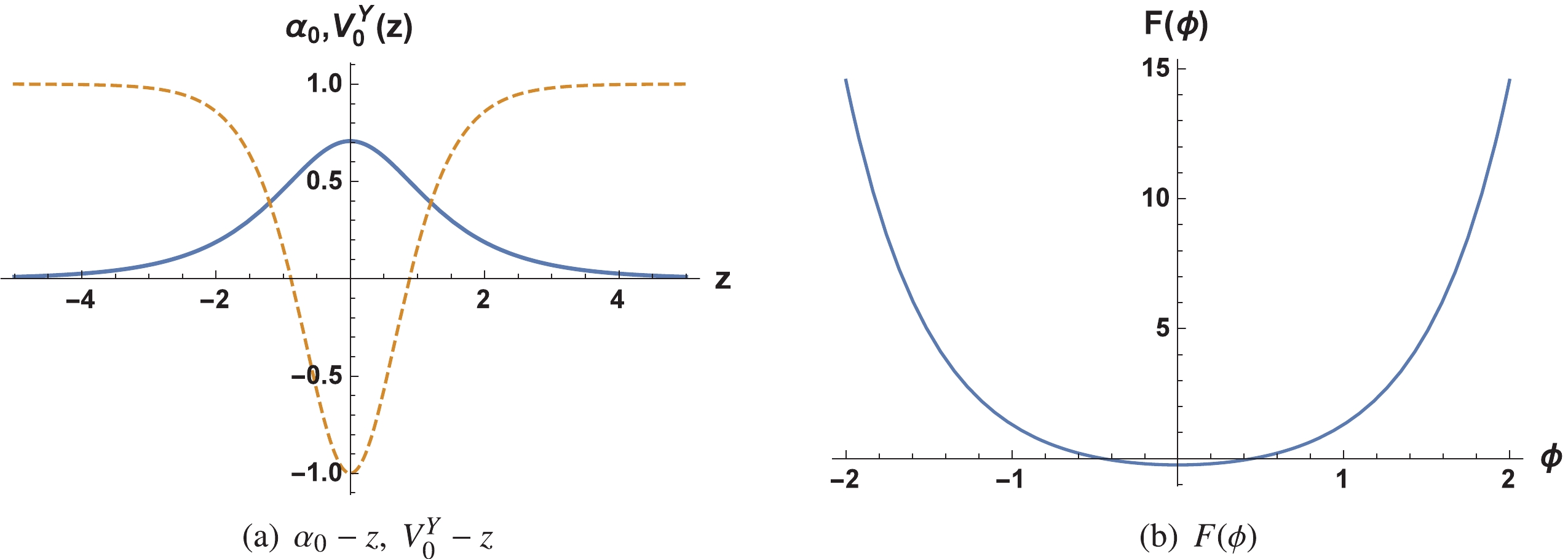
Figure 1. (color online) Shapes of the Elko zero mode
$\alpha_{0}(z)$ according to Eq. (51) (thick line); the effective potential$V^Y_0(z)$ (dashed line) is plotted on the left and the shape of function$F(\phi)$ according to Eq. (52) (right) is plotted on the right. The parameters were set to$h=b=p=\eta=a^2s(1 + \Lambda_4)=1$ . -
Next, we focus on the non-minimal coupling mechanism. As shown in a previous study of ours [97], there exist different configurations of the Elko zero mode and
$ f(\phi) $ for different choices of$ K(z) $ . In this paper, we consider two types of$ K(z) $ and investigate the localization of the Elko zero mode according to Eq. (40). -
First, a natural choice implies
$ K(z) = -kA' $ with$ k $ being a positive constant. Thus, it is easy to obtain$ C(z) = \frac{1}{\mathcal{C}_1\cosh(hz)^{-k}-\dfrac{\coth(hz)\mathcal{F}(z)\sqrt{-\sinh^2(hz)}}{h+hk}}. $

(55) Here
$ \mathcal{F}(z) = {}_{2}\text{F}_{1}\left(\dfrac{1}{2},\dfrac{1+k}{2};\dfrac{3+k}{2};\cosh^2(hz)\right) $ . Especially, when$ k = 1 $ , the form of$ C(z) $ is reduced to$ C(z) = \frac{h\cosh(h z)}{h\mathcal{C}_1-\sinh(hz)}.$

(56) Here
$ \mathcal{C}_1 $ is an arbitrary constant and we set$ \mathcal{C}_1 = 0 $ . Thus, the zero mode is rewritten as$ \begin{aligned}[b] \alpha_{0}(z)\varpropto &\;\text{e}^{D(z)} = {\exp}\left[\frac{1}{2}\int^{z}_{0}\frac{A'^2}{C}{\rm d}\bar{z}\right]{\exp}\left[-\frac{1}{2}\int^{z}_{0}K{\rm d}\bar{z}\right]\\ \varpropto&\;\text{sech}(hz){\exp}\left[-\frac{1}{4}\text{sech}^2(hz)\right]. \end{aligned} $

(57) It is easy to check that the orthonormality condition
$\begin{aligned}[b]\int \alpha^*_0\alpha_0{\rm d}z = \int \alpha_0^2{\rm d}z\varpropto\int \text{sech}^2(h\bar{z}){\rm d}z\end{aligned}$

$\begin{aligned}[b]{\exp}\Bigg[-\frac{1}{2}\text{sech}^2(h\bar{z})\Bigg] = 2\sqrt{2}F({\sqrt{2}}/{2})<\infty \end{aligned}$

(58) can be satisfied. Here,
$ F(z) $ gives the Dawson integral and$ F({\sqrt{2}}/{2}) = 0.512496 $ . In this case, the effective potential$ V_0^N(z) $ is given by$\begin{aligned}[b] V_0^N(z) =& \frac{h^2}{32}(-2-5\cosh(2hz)-10\cosh(4hz)\\&+\cosh(6hz))\text{sech}^6(hz). \end{aligned} $

(59) The function
$ f(\phi) $ reads$\begin{aligned}[b] f(\phi(z)) =& \frac{a^4s^2}{h^2}(1 + \Lambda_4)^2\cosh^3(b\phi)\tanh^2(b\phi)\; \\&\times{\exp}\left[-\frac{1}{2}\text{sech}^2(b\phi)\right]. \end{aligned} $

(60) We present the shapes of the zero mode, the effective potential, and the coupling function in Fig. 2. Note from Fig. 2 (a) that the zero mode defined in Eq. (57) is localized on the brane and the effective potential is a PT-type one. It is evident that the shape of
$ f(\phi) $ is similar to that of$ F(\phi) $ shown in the previous subsection: it has a minimum at the point$ \phi = 0 $ and diverges at infinity. Given that there exists a factor$ \text{e}^{-3A} $ in the expression of$ f(\phi) $ defined in Eq. (41), the boundary behaviour of$ f(\phi) $ is also opposite to the warp factor as well as to$ F(\phi) $ . This also ensures that the action of Eq. (27) does not diverge and the brane model is stable.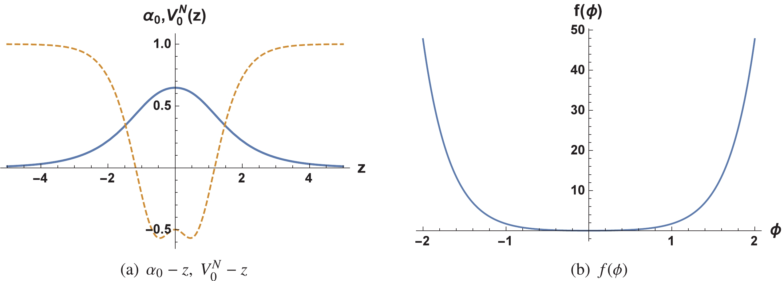
Figure 2. (color online) Shapes of the Elko zero mode
$\alpha_{0}(z)$ according to Eq. (57) (thick line); the effective potential$V_0^N(z)$ in Eq. (59) (dashed line) is plotted on the left and the shape of function$f(\phi)$ according to Eq. (60) (right) is plotted on the right. The parameters were set to$h=b=a^2s(1 + \Lambda_4)=1$ . -
Another natural choice for
$ K(z) $ is$ K(z) = k\phi = k\dfrac{h}{b}z $ with positive$ k $ . In this case, the form of$ C(z) $ reads$ C(z) = -\frac{\sqrt{\dfrac{2\bar{k}}{\pi}}}{\text{Erfi}\left(\sqrt{\dfrac{\bar{k}}{2}}z\right)}\text{e}^{\frac{\bar{k}}{2}z^2}, $

(61) where
$\bar{k}\equiv k\dfrac{h}{b}$ and$\text{Erfi}\big(\sqrt{{\bar{k}}/{2}}z\big)$ is the imaginary error function. Thus, the zero mode reads$ \alpha_{0}(z)\varpropto {\exp}\left[-\frac{1}{2} h^2 \sqrt{\frac{\pi}{2\bar{k}}}\; \mathcal{L}(z) -\frac{\bar{k}}{4}z^{2}\right] $

(62) with
$ \mathcal{L}(z)\equiv \int^{z}_{0} \text{Erfi} \left(\sqrt{\frac{\bar{k}}{2}}\bar{z}\right) \tanh^2(h\bar{z}){\exp} \left[\frac{-\bar{k} \bar{z}^{2}}{2}\right] {\rm d}\bar{z}.\; \; \; \; $

(63) It can be verified that the function
$ \mathcal{L}(z) $ approaches a constant as$ |z|\rightarrow \infty $ , which indicates that$ \alpha_0(|z|\rightarrow \infty)\varpropto $ $ {\exp}\left[-\dfrac{\bar{k}}{4}z^{2}\right] $ and its orthonormality condition can be satisfied.The zero mode in this case can be localized on the brane shown in Fig. 3 (a). Given that the effective potential
$ V_0^N(z) $ and the corresponding coupling function$ f(\phi) $ have slightly complex forms, only their shapes are displayed in Fig. 3. Note from Fig. 3 (a) that the effective potential is an infinite deep potential instead of a PT-type one. The behaviour of$ f(\phi) $ in Fig. 3 (b) is still similar to the ones in the previous two subsections. Therefore, the functions$ F(\phi) $ and$ f(\phi) $ have similar properties and play similar roles, although they appear in different places in the actions.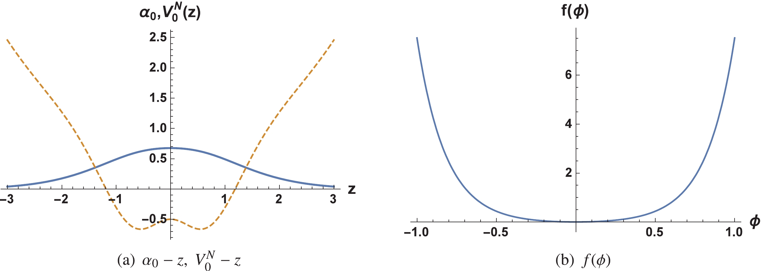
Figure 3. (color online) Shapes of the Elko zero mode
$\alpha_{0}(z)$ according to Eq. (62) (thick line); the effective potential$V_0^N(z)$ (dashed line) is plotted on the left and the shape of function$f(\phi)$ (right) is plotted on the right. The parameters were set to$\bar{k}=h=b=a^2s(1 + \Lambda_4)=1$ . -
In this section, we consider another type of AdS thick brane model and investigate the localization of the Elko zero mode with two types of couplings. The warp factor in the previous section is convergent as
$ z\rightarrow \infty $ or$ y\rightarrow \infty $ , but the one in this section diverges, which means that the zero mode of a five-dimensional free scalar field cannot be localized on this brane [56]. This difference leads to different and interesting results.The action of this system reads [56]
$ S = \int {\rm d}^5 x \sqrt{-g}\left[\frac{1}{2} R-\frac{1}{2} g^{MN}\partial_M \phi \partial_N \phi - V(\phi) \right], $

(64) where
$ R $ is the five-dimensional scalar curvature. Note that$ M_5 $ is set to 2 here. The metric is described by Eq. (3) and the induced metric is$ \hat{g}_{\mu\nu} = {\rm e}^{-2\beta x_3}(-{\rm d}t^2+{\rm d}x_1^2+{\rm d}x_2^2)+ $ $ {\rm d}x_3^2 $ with$ \Lambda_4 = -3\beta^2 $ . For the scalar potential$ V(\phi) = -\frac{3(1+3\delta)\beta^{2}}{2\delta}\cosh^{2(1-\delta)} \left(\frac{\phi}{\phi_{0}} \right), $

(65) a thick AdS brane solution was given in Refs. [24, 56]:
$ A(z) = -\delta\ln\left|\cos \left(\frac{\beta}{\delta}z\right) \right|,$

(66) $ \phi(z) = \phi_{0}\text{arcsinh}\left(\tan\left(\frac{\beta}{\delta}z\right)\right) $

(67) with
$ \phi_{0}\equiv\sqrt{3\delta(\delta-1)}. $

(68) Here, the range of the extra dimension is
$ -z_{b}\leqslant z\leqslant z_{b} $ with$ z_{b} = \left|\dfrac{\delta\pi}{2\beta}\right| $ ; the parameter$ \delta $ satisfies$ \delta >1 $ or$ \delta <0 $ . It was found that only when$ \delta>1 $ , there exists a thick 3-brane that localizes at$ |z|\approx0 $ [24, 56]. Thus, we only consider the case$ \delta>1 $ . In this case, the warp factor$ \text{e}^{2A(z)} $ diverges at the boundaries$ z = \pm z_{b} $ . -
Using the Yukawa-like coupling and substituting Eqs. (66) and (67) into (23)-(26), the Elko zero mode
$ \alpha_0 $ , the function$ F(\phi) $ , and the effective potential$ V_0^{Y} $ respectively read$ \alpha_0\propto\text{e}^{pA(z)} = \cos^{-p\delta}\left(\frac{\beta}{\delta}z\right), $

(69) $ \begin{aligned}[b] F(\phi) =& \frac{\beta^2}{8\delta\beta}\Bigg[6-4p+(6+13\delta\\&-4p(1+p\delta))\sinh^2\left(\frac{\phi}{\phi_0}\right)\Bigg]\\&\times\cosh^{-2\delta}\left(\frac{\phi}{\phi_0}\right),\end{aligned} $

(70) $ V_0^Y = p A'' + p^2A'^2 = \frac{p\beta^2}{\delta}\sec^2\left(\frac{\beta}{\delta}z\right)+p^2\beta^2\tan^2\left(\frac{\beta}{\delta}z\right). $

(71) The orthonormality condition requires
$ p\delta<0 $ :$ \begin{aligned}[b]\int \alpha^*_0\alpha_0{\rm d}z =& \int \alpha_0^2{\rm d}z\propto\int^{\frac{\delta\pi}{2\beta}}_{-\frac{\delta\pi}{2\beta}} \cos^{-2p\delta}\left(\frac{\beta}{\delta}z\right){\rm d}z\\ =& \frac{\sqrt{\pi}\Gamma\left(\dfrac{1}{2}-p\delta\right)}{\Gamma(1-p\delta)}<\infty. \end{aligned} $

(72) Therefore, the zero mode can be localized on this AdS thick brane for any negative
$ p $ by introducing the Yukawa-like coupling mechanism.The zero mode, effective potential
$ V_0^Y(z) $ , and function$ F(\phi) $ are plotted in Fig. 4. A unique point to be remarked is that the effective potential is an infinite potential well and the behaviour of$ F(\phi) $ is a volcano-type one, which is due to the opposite boundary behavior of the warp factor compared to that of the previous section.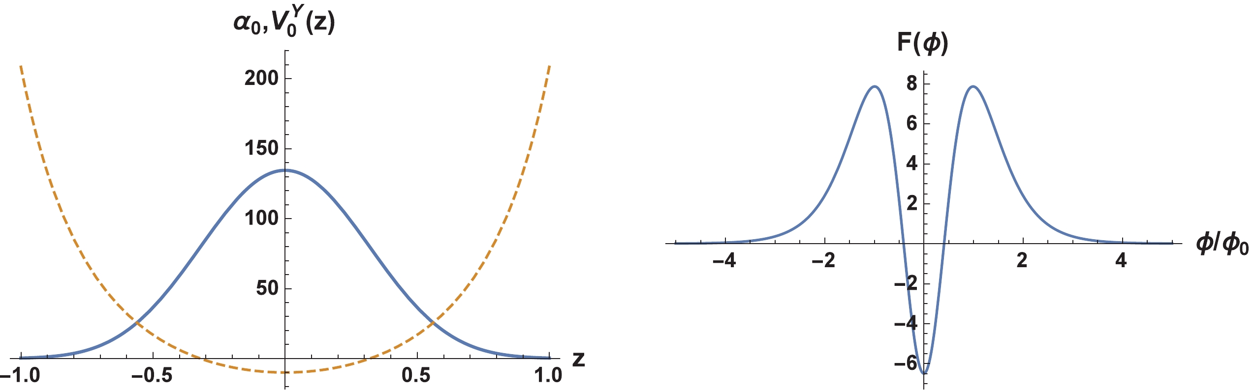
Figure 4. (color online) Shapes of the Elko zero mode
$\alpha_{0}(z)$ according to Eq. (69) (thick line); the effective potential$V^Y_0(z)$ according to Eq. (71) (dashed line) is plotted on the left and the shape of function$F(\phi)$ according to Eq. (70) (right) is plotted on the right. For the sake of better visibility, here$\alpha_{0}(z)$ has been magnified 100 times. The parameters were set to$\eta=-1$ ,$\delta=\beta=2$ , and$p=-5$ . -
Finally, we turn to the non-minimal coupling mechanism by considering
$ K(z) = kA' $ with$ k $ a positive constant. Note that the sign in front of$ k $ is just opposite to that in the previous section. When$ k = \dfrac{1}{\delta} $ , Eq. (42) can be rewritten as$ C(z) = { \frac{\bar{k}\sec(\bar{k}z)} {\ln\left(\dfrac{\cos\left(\dfrac{\bar{k}}{2}z\right) -\sin\left(\dfrac{\bar{k}}{2}z\right)} {\cos\left(\dfrac{\bar{k}}{2}z\right) +\sin\left(\dfrac{\bar{k}}{2}z\right)} \right)} },$

(73) where
$ \bar{k}\equiv\dfrac{\beta}{\delta} $ and the parameter$ \mathcal{C}_1 $ is set to zero. Then, the zero mode reads$\alpha_{0}(z)\varpropto \cos^{1/2}(\bar{k}z)\; {\exp} \left[\frac{1}{2}\bar{k}\delta^2 \int^{z}_{0} \sin(\bar{k}\bar{z})\tan(\bar{k}\bar{z})\ln\left(\frac{\cos\left(\dfrac{\bar{k}}{2}\bar{z}\right) -\sin\left(\dfrac{\bar{k}}{2}\bar{z}\right)} {\cos\left(\dfrac{\bar{k}}{2}\bar{z}\right) +\sin\left(\dfrac{\bar{k}}{2}\bar{z}\right)} \right) {\rm d}\bar{z} \right]. $ 
(74) It is easy to check that in this case the zero mode will vanish when
$ z\rightarrow \pm z_{b} $ and the orthonormality condition can also be satisfied. As shown in Fig. 5, the zero mode is localized on the brane. The effective potential is an infinite deep potential well, and the coupling function$ f(\phi) $ is the volcano-type one. Note that all of the coupling functions ($ F(\phi) $ and$ f(\phi) $ ) have a minimum at$ \phi = 0 $ in both thick brane models.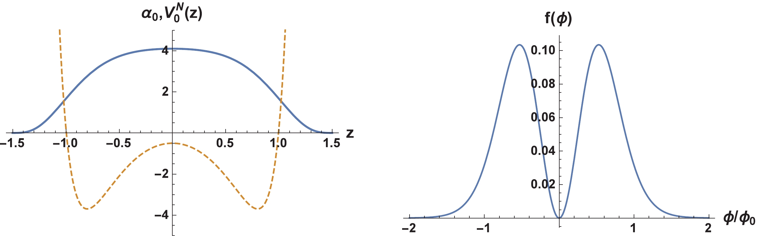
Figure 5. (color online) Shapes of the Elko zero mode
$\alpha_{0}(z)$ according to Eq. (74) (thick line); the effective potential$V^N_0(z)$ (dashed line) is plotted on the left and the shape of function$f(\phi)$ (right) is plotted on the right. For better visibility,$\alpha_{0}(z)$ has been magnified 5 times. The parameters were set to$\beta=\delta=2$ . -
In this study, we introduced two types of localization mechanism to investigate the localization of the five-dimensional Elko zero mode on dS/AdS thick branes. First, we reviewed two coupling mechanisms, i.e, the Yukawa-like coupling and the non-minimal coupling. The results indicate that to obtain the Elko zero mode on a brane, the form of
$ F(\phi) $ in the Yukawa-type coupling mechanism must be determined by the warped factor as described in Eq. (24), and the function$ f(\phi) $ in the non-minimal coupling mechanism should be determined by the introduced auxiliary function$ K(z) $ . Then, we considered two types of curved thick brane models and investigated the localization of the Elko zero mode with both types of localization mechanism.In the first brane model with convergent warp factor, we considered the dS/AdS thick brane generated by a single scalar field. The results are as follows:
● For the Yukawa-like coupling,
1. the zero mode can be localized on branes under the condition
$ p>0 $ ;2. the effective potential is a PT-type one;
3. the coupling function of
$ F(\phi) $ has the opposite boundary behavior compared to the warp factor$ \text{e}^{2A} $ ;$ F(\phi) $ diverges when$ \phi\rightarrow \infty $ and it has a minimum at$ \phi = 0 $ .● For the non-minimal coupling, by introducing two different forms of the auxiliary function
$ K(z) $ ,1. the zero mode can be confined on branes;
2. in one case, the effective potential is a PT-type one; in another case, it is an infinity deep potential well;
3. the behaviors of
$ f(\phi) $ in both two cases are similar to that of$ F(\phi) $ :$ \; \; f(\phi)\rightarrow \infty $ as$ \phi\rightarrow \infty $ and it also has a minimum at$ \phi = 0 $ .In another AdS thick brane model with the divergent warp factor, the results are as follows:
● both the zero modes in two coupling mechanisms can be confined on branes; while for the Yukawa-type coupling, the range of the parameter
$ p $ in this model is expanded and it can take any negative value;● the effective potential in the two coupling mechanisms is an infinity deep potential well;
● the coupling functions of
$ F(\phi) $ and$ f(\phi) $ are both volcano-type.In short, regardless of the coupling mechanism considered, the Elko zero mode could be confined on dS/AdS thick branes and the roles of coupling functions (
$ F(\phi) $ and$ f(\phi) $ ) were the same. These results may provide a new perspective to explore more localization mechanisms and expand the possibility of localizing the Elko spinor.In this paper, we report the expressions of the coupling functions to localize the five-dimensional Elko zero mode on dS/AdS thick branes. We found that the effective potential in the Schrödinger-like equation for the zero mode is a PT-type one or an infinite deep potential well. However, note that the Schrödinger-like equation for the massive KK modes is a complex one, which is notably different from that for the zero mode. Thus, the effective potential function reported in this paper is not applicable for the massive KK modes. Moreover, we cannot judge whether there exists a massive KK mode, although the effective potential is a PT-type one or an infinite deep potential well. In the future, we will investigate the localization of the massive Elko KK modes on different thick branes.
-
The authors thank Professor Yu-Xiao Liu for his kind help.
Localization of five-dimensional Elko spinors on dS/AdS thick branes
- Received Date: 2021-08-26
- Available Online: 2022-02-15
Abstract: Owing to the special structure of a five-dimensional Elko spinor, its localization on a brane with codimension one becomes completely different from that of a Dirac spinor. By introducing the coupling between the Elko spinor and the scalar field that can generate the brane, we have two types of localization mechanism for the five-dimensional Elko spinor zero mode on a brane. One is the Yukawa-type coupling, and the other is the non-minimal coupling. In this study, we investigate the localization of the Elko zero mode on de Sitter and Anti-de Sitter thick branes with the two localization mechanisms, respectively. The results show that both the mechanisms can achieve localization. The forms of the scalar coupling function in both localization mechanisms have similar properties, and they play a similar role in localization.


 DownLoad: