


 Abstract
 HTML
HTML Reference
 Related
 PDF
PDF


-
For a theoretical scientist, radial excited hadrons are more challenging to study than their ground states. They are widely studied in the quark model [1-6]. However, many “missing states” have been predicted. A more rigorous corresponding relation between the quark model resonant states and the experimental observed ones is expected. Lattice Quantum Chromodynamics (QCD) aims to produce the hadron spectrum from first principle. The study of radial excited states is also less advanced than that of the ground states; see Table I and Table II in Ref. [7] for a lattice QCD study of ground state mesons. For the radial excited hadrons, see Ref. [8-13].
My purpose herein is to study the radial excited states via a continuum QCD approach, the Dyson-Schwinger equation and the Bethe-Salpeter equation (DSBSE) approach. Many interesting properties of the excited states have been obtained using this approach, for example, the radial excited pseudoscalar mesons decouple from the axial-vector current in the chiral limit [14]. The electromagnetic properties and chiral symmetry restoration of the radial excited states were also studied [15, 16]. It is shown qualitatively that radial excited mesons are more sensitive to interactions at a large distance, though a realistic prediction for the excited mesons from the rainbow ladder (RL) approximation failed [17, 18].
In this paper, I focus on the the first radial excited heavy pseudoscalar and vector mesons, i.e.
$ \eta_c(2S) $ ,$ \psi(2S) $ ,$ B_c(2S) $ ,$ B^*_c(2S) $ ,$ \eta_b(2S) $ and$ \varUpsilon(2S) $ . Of these mesons,$ \psi(2S) $ and$ \varUpsilon(2S) $ were discovered more than 20 years ago [19, 20], and they were extensively studied in the following years. Even so, the decay width of$ \eta_b(2S) $ is not well determined. Then,$ \eta_c(2S) $ was discovered in 2004 [21] and$ \eta_b(2S) $ in 2012 [22]. The$ B_c $ mesons are much more difficult to observe due to their small production cross sections. Until recently,$ B_c(2S) $ and$ B^*_c(2S) $ were measured by the CMS and LHCb collaborations [23, 24], yet the mass of$ B^*_c(2S) $ has not been determined precisely. Therefore, a systematic theoretical study of these mesons is of significant meaning.I and my collaborators studied these excited mesons in the RL approximation in Ref. [25]. Therein, one gluon exchange effective interaction between a quark and an antiquark is fixed by the ground state mesons [7]. The effective interaction in Ref. [7] is universal for all light, heavy-light, and heavy ground pseudoscalar and vector mesons. It could be extended to ground state scalar and axial vector mesons [26]. When applying the same interaction to radial excited heavy mesons, we found that the spectrum is 1% lower than the available experimental value. The leptonic decay constant is lower by 12% for
$ \varUpsilon(2S) $ and by 42% for$ \psi(2S) $ . This tells us that radial excited mesons do not share the same effective interactions with ground state mesons.What should an effective interaction be like? A proper interaction should not only produce the right spectrum, but also the right wave function for the mesons. The leptonic decay constant (see Eq. (3) and Eq. (4)) describes quark antiquark annihilation inside a meson and thus, is the simplest quantity related to the meson wave function. Therefore, herein I refix the effective interaction with the masses and leptonic decay constants of
$ \varUpsilon(2S) $ and$ \psi(2S) $ . Then, the masses and leptonic decay constants of the other four resonances are calculated. It turns out that all first radial excited heavy pseudoscalar and vector mesons could be described in a universal effective interaction. In Section II, I introduce the framework of the DSBSE approach in the RL approximation. The details of the calculation and the results are expounded in Section III. Finally, the summary and conclusions are given in Section IV. -
The framework has been introduced in previous works [7, 25, 26]. It is recapitulated here for convenience. In the RL approximation, the quark propagator is solved by the Gap equation [27, 28]:
$ S_f^{-1}(k) = Z_2 ({\rm i}\gamma\cdot k + Z_m m_f) + \frac{4}{3} (Z_2)^2 \int^\Lambda_{{\rm d} q} \tilde{D}^f_{\mu\nu}(l)\gamma_\mu S_{f}(q)\gamma_\nu, $

(1) where
$ f = \{u,d,s,c,b,t\} $ represents the quark flavor.$ S_{f}(k) $ is the quark propagator, which can be decomposed as$ S_{f}(k) = \dfrac{Z_f(k^2)}{{\rm i}{\not{k}} + M_f(k^2)} $ .$ Z_f(k^2) $ is the quark dressing function and$ M_f(k^2) $ the quark mass function.$ l = k-q $ .$ m_f $ is the current quark mass.$ \tilde{D}^f_{\mu\nu} $ represents the effective interaction for the self energy of the f-quark.$ Z_2 $ and$ Z_m $ are the renormalisation constants of the quark field and the quark mass, respectively.$ \int^\Lambda_{{\rm d} q} = \int ^{\Lambda} {\rm d}^{4} q/(2\pi)^{4} $ stands for a Poincar$ \acute{\text{e}} $ invariant regularized integration, with the regularization scale Λ .A meson is qualified by the Bethe-Salpeter amplitude (BSA),
$ \Gamma^{fg}(k;P) $ , with k and P being the relative and the total momentum of the meson, respectively.$ P^2 = -M^2_{fg} $ , and$ M_{fg} $ is the mass of the meson with quark flavor$ (f,g) $ . The BSA is solved by the Bethe-Salpeter equation (BSE) [29, 30]$ \Big{[} \Gamma^{fg}(k;P) \Big{]}^{\alpha}_{\beta} = - \int^\Lambda_{{\rm d} q} \frac{4}{3}(Z_{2})^{2} \tilde{D}^{fg}_{\mu\nu}(l) \Big[\gamma_{\mu}^{}\Big]^{\alpha}_\sigma \Big[\gamma_{\nu}\Big]^\delta_\beta \Big{[} \chi^{fg}(q;P) \Big{]}^{\sigma}_{\delta} , $

(2) where α, β, σ, and δ are the Dirac indexes.
$ \chi^{fg}(q;P) = S_{f}(q_{+}) \Gamma^{fg}(q;P) S_{g}(q_{-}) $ is the wave function,$ q_{+} = q + \eta P/2 $ ,$ q_{-} = q - (1-\eta) P/2 $ , η is the partitioning parameter describing the momentum partition between the quark and the antiquark and does not affect the physical observables.$ \tilde{D}^{fg}_{\mu\nu} $ represents the effective interaction between the quark and the antiquark. The leptonic decay constant of the pseudoscalar meson,$ f_{0^{-}} $ , is obtained by$ f_{0^-}P_{\mu} = Z_{2} N_{c} \;\text{tr} \int^{\Lambda}_{{\rm d} q} \gamma_{5}^{} \gamma_{\mu}^{} S_f(q_+)\Gamma^{fg}_{0^-}(q;P)S_g(q_-). $

(3) $ N_c = 3 $ , is the color number. “$ \text{tr} $ ” represents the trace of the Dirac index. The leptonic decay constant of the vector meson,$ f_{1^{-}} $ , is analogous to$ f_{1^-}M_{1^-} = Z_{2} N_{c} \;\text{tr} \int^{\Lambda}_{{\rm d} q} \gamma_{\mu}^{} S_f(q_+)\Gamma^{fg,\mu}_{1^-}(q;P)S_g(q_-). $

(4) $ \tilde{D}^{f}_{\mu\nu} $ and$ \tilde{D}^{fg}_{\mu\nu} $ are decomposed as$ \tilde{D}^{f}_{\mu\nu}(l) = \left(\delta_{\mu\nu}-\dfrac{l_{\mu}l_{\nu}}{l^{2}}\right) $ $ {\cal{G}}^f(l^2) $ and$ \tilde{D}^{fg}_{\mu\nu}(l) = \left(\delta_{\mu\nu}-\dfrac{l_{\mu}l_{\nu}}{l^{2}}\right){\cal{G}}^{fg}(l^2) $ . The dressing functions$ {\cal{G}}^f(l^2) $ and$ {\cal{G}}^{fg}(l^2) $ are modeled as$ {\cal{G}}^f(s) = {\cal{G}}^f_{IR}(s) + {\cal{G}}_{UV}(s), $

(5) $ {\cal{G}}^f_{IR}(s) = 8\pi^2\frac{D_f^2}{\omega_f^4} {\rm e}^{-s/\omega_f^2}, $

(6) $ {\cal{G}}^{fg}(s) = {\cal{G}}^{fg}_{IR}(s) + {\cal{G}}_{UV}(s), $

(7) $ {\cal{G}}^{fg}_{IR}(s) = 8\pi^2\frac{D_f}{\omega_f^2}\frac{D_g}{\omega_g^2} {\rm e}^{-s/(\omega_f\omega_g)}, $

(8) $ {\cal{G}}_{UV}(s) = \frac{8\pi^{2} \gamma_{m}^{} {\cal{F}}(s)}{\text{ln}\big[\tau+(1+s/\Lambda^{2}_{\rm QCD})^2\big]}, $

(9) where
$ s = l^2 $ .$ {\cal{G}}^f_{IR}(s) $ and$ {\cal{G}}^{fg}_{IR}(s) $ are the infrared interactions responsible for the hadron properties.$ \omega_f $ represents the interaction width in momentum space, and$ D_f $ is the infrared strength.$ {\cal{G}}_{UV}(s) $ keeps the one-loop perturbative QCD limit in the ultraviolet.$ {\cal{F}}(s) = [1 - \exp(-s^2/ $ $ [4m_{t}^{4}])]/s $ ,$ \gamma_{m}^{} = 12/(33-2N_{f}) $ , with$ m_{t} = 1.0 \;{\rm{ GeV}}\, $ ,$ \tau = e^{10} - 1 $ ,$ N_f = 5 $ , and$ \Lambda_{\text{QCD}} = 0.21 \;{\rm{ GeV}}\, $ . This model turned out to be successful for all ground state pseudoscalar and vector mesons, from heavy, heavy-light to light mass scales. It has been extended to the scalar and axial vector mesons [26]. These successes support that Eq. (8) contains the proper flavor dependence. However, the same interaction should not apply to radial excited mesons if high precision is required, as stated in Section I.To mimic the interesting difference between the radial excited states and the ground states, Eq. (8) is changed into
$ {\cal{G}}^{fg}_{IR}(s) = 8\pi^2\frac{\eta_f D_f}{\omega_f^2}\frac{ \eta_ g D_g}{\omega_g^2} {\rm e}^{-s/(\alpha_f\omega_f \alpha_g\omega_g)}. $

(10) While
$ \omega_f $ and$ D_f $ ($ f = \{c,b\} $ ) are kept unchanged from those in Ref. [7],$ \alpha_f $ and$ \eta_f $ ($ f = \{c,b\} $ ) are free parameters.$ \alpha_f $ presents the changing of the interaction width and$ \eta_f $ the infrared strength. The four free parameters,$ \alpha_c $ ,$ \alpha_b $ ,$ \eta_c $ , and$ \eta_b $ , are fixed by fitting the masses and leptonic decay constants of$ \psi(2S) $ and$ \varUpsilon(2S) $ ($ M_{\psi(2S)} $ ,$ M_{\varUpsilon(2S)} $ ,$ f_{\psi(2S)} $ ,$ f_{\varUpsilon(2S)} $ ) to the experimental values. The exprimental values of$ f_{\psi(2S)} $ and$ f_{\varUpsilon(2S)} $ are extracted from the branch decay width of the vector meson to$ e^+ e^- $ . The values are$ f_{\psi(2S)} = -0.208\;{\rm{ GeV}} $ ,$ f_{\varUpsilon(2S)} = -0.352\;{\rm{ GeV}} $ [25]. Then, the masses and leptonic decay constants of$ \eta_c(2S) $ ,$ B_c(2S) $ ,$ B^*_c(2S) $ , and$ \eta_b(2S) $ are calculated with refixed interactions. -
Before discussing the results, we should first explain the process of solving the BSE, Eq. (2). Eq. (2) is solved as a
$ P^{2} $ -dependent eigenvalue problem,$ \lambda^{fg}(P^2) \Big{[} \Gamma^{fg}(k;P) \Big{]}^{\alpha}_{\beta} = - \int^\Lambda_{{\rm d} q} \frac{4}{3}(Z_{2})^{2} \tilde{D}^{fg}_{\mu\nu}(l) \Big[\gamma_{\mu}^{}\Big]^{\alpha}_\sigma \Big[\gamma_{\nu}\Big]^\delta_\beta \Big{[} \chi^{fg}(q;P) \Big{]}^{\sigma}_{\delta}. $

(11) The meson mass is determined by
$ \lambda^{fg}(P^2 = -M^2_{fg}) = 1 $ . However, due to the singularity of the quark propagators in the complex momentum plane, there is a lower bound value for$ P^2 $ in Eq. (11). Only when$ P^2 > -M_{\rm max}^2 $ , Eq. (11) is solvable.$ M_{\rm max}^2 $ defines the contour border of the calculable region of the quark propagators; see appendix of Ref. [31] for this problem.As the masses of the radial excited mesons are beyond the contour border, i.e.
$ M_{fg} > M_{\rm max} $ , the following form is used to fit$ \lambda^{fg}(P^2) $ :$ \frac{1}{\lambda^{fg}(P^2)} = \frac{1 + \displaystyle\sum^{N_{o}}_{n = 1}\, a_{n} (P^{2} + s_{0}^{})^n}{1 + \displaystyle\sum^{N_{o}}_{n = 1}\, b_{n} (P^{2} + s_{0}^{})^n} \, , $

(12) where
$ N_{o} $ is the order of the series$ s_{0}^{} $ , and$ a_{n} $ and$ b_{n} $ are the parameters to be determined by the least square method.$ f_{fg}(P^2) $ is fitted by$ f_{fg}(P^2) = \frac{f_0 + \displaystyle\sum^{N_o}_{n = 1}\, c_n (P^2+M^2)^n}{1 + \displaystyle\sum^{N_o}_{n = 1}\, d_n (P^2+M^2)^n}, $

(13) where
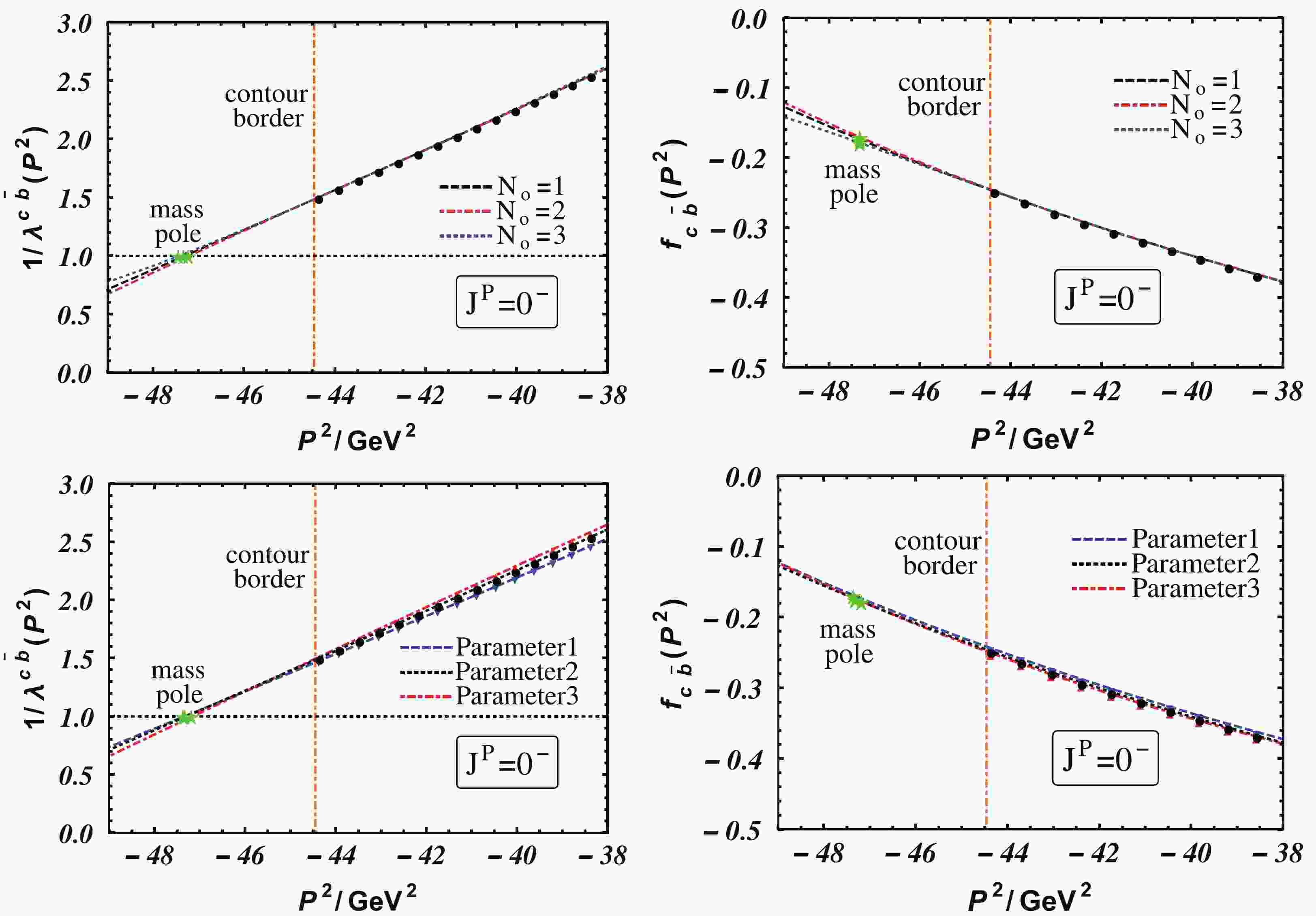
$ f_{0}^{} $ ,$ c_{n} $ , and$ d_{n} $ are parameters, and$ M^{2} $ is the square of the mass. The physical value of the decay constant is$ f_{fg}(-M^2) = f_{0}^{} $ . This extrapolation scheme has been used in Refs. [25, 26]. The error is controllable as long as the physical mass of the meson is not considerably larger than$ M_{\rm max} $ . The extrapolation results are illustrated by$ B_c(2S) $ in the two upper figures of Fig. 1.$ N_o = 1, 2, 3 $ are considered in practice, and the differences between the three cases are estimated to be the error from extrapolation.
Figure 1. (color online) Extrapolation of the eigenvalue,
$\lambda(P^2)$ , and the leptonic decay constant,$f(P^2)$ , of$B_c(2S)$ . The upper two figures show the extrapolation with$N_o = 1, 2, 3$ using Eq. (12) and Eq. (13). The lower two figures show the results of using the three different groups of parameters that are listed in Table A1 in the appendix. The vertical dot-dashed orange line is the contour border on the right of which the direct calculation can be applied. The green stars present the location of the meson masses.Three groups of
$ \omega_f $ and$ D_f $ are used, which are the same as in Ref. [7]. Different groups of parameters correspond to different interaction widths. In each case,$ \alpha_f $ and$ \eta_f $ ($ f = \{c,b\} $ ), are fixed by fitting the masses and leptonic decay constants of$ \psi(2S) $ and$ \varUpsilon(2S) $ to the experimental values. Then, masses and leptonic decay constants of$ \eta_c(2S) $ ,$ B_c(2S) $ ,$ B^*_c(2S) $ , and$ \eta_b(2S) $ are outputted. The differences in the outputs are considered to be the errors due to varying the parameters. This is illustrated by$ B_c(2S) $ , the two lower figures of Fig. 1.The masses and leptonic decay constants of
$ \eta_c(2S) $ ,$ \psi(2S) $ ,$ B_c(2S) $ ,$ B^*_c(2S) $ ,$ \eta_b(2S) $ , and$ \varUpsilon(2S) $ herein (the DSE results) and the available experimental values (the expt. results) are listed in Table 1. For the DSE results, the first error is from the extrapolation, and the second is from varying the parameters. The extrapolation errors of the charmonium masses are larger than those of the$ B_c $ mesons and the bottomonium, because heavier mesons are less affected by the higher orders in Eq. (12) in the extrapolation process. Comparing the DSE results with the experimental values, the largest mass deviation is$ 20\;{\rm{ MeV}} $ , in the case of$ \eta_c(2S) $ . Therefore, the systematic error of the DSE calculated spectrum is estimated to be$ 20\;{\rm{ MeV}} $ . The mass of$ B^*_c(2S) $ is not well determined experimentally, due to a lack of knowledge of the$ B^*_c(1S) $ mass. Herein, I provide the most precise prediction of the$ B^*_c(2S) $ mass to date. Note that my prediction is also consistent with the potential model results, for example, see Table IV in Ref. [37].meson $J^{\text{PC}}$ 

$M^{\text{DSE}}_{c\bar{c}}$ 

$M^{\text{expt.}}_{c\bar{c}}$ 

$f^{\text{DSE}}_{c\bar{c}}$ 

$f^{\text{expt.}}_{c\bar{c}}$ 

$|f|$ [33]

$|f|$ [36]

$\eta_c(2S)$ 

$0^{-+}$ 

3.618(25)(3) 3.638 −0.158(8)(4) − 0.170~0.172 0.197 $\psi(2S)$ 

$1^{--}$ 

3.686(21)(0) 3.686 −0.208(5)(0) −0.208 0.207~0.216 0.182 meson $J^{\text{P}}$ 

$M^{\text{DSE}}_{c\bar{b}}$ 

$M^{\text{expt.}}_{c\bar{b}}$ 

$f^{\text{DSE}}_{c\bar{b}}$ 

$f^{\text{expt.}}_{c\bar{b}}$ 

$|f|$ [34]

$|f|$ [35]

$|f|$ [36]

$B_c(2S)$ 

$0^{-}$ 

6.874(9)(6) 6.872 −0.174(5)(4) − $0.198(35)$ 

0.304(14) 0.251 $B^*_c(2S)$ 

$1^{-}$ 

6.926(12)(6) − −0.216(9)(4) − − 0.325(14) 0.252 meson $J^{\text{PC}}$ 

$M^{\text{DSE}}_{b\bar{b}}$ 

$M^{\text{expt.}}_{b\bar{b}}$ 

$f^{\text{DSE}}_{b\bar{b}}$ 

$f^{\text{expt.}}_{b\bar{b}}$ 

$|f|$ [33]

$|f|$ [36]

$\eta_b(2S)$ 

$0^{-+}$ 

9.989(13)(3) 9.999 −0.345(6)(1) − 0.291~0.299 0.367 $\varUpsilon(2S)$ 

$1^{--}$ 

10.023(11)(0) 10.023 -0.352(4)(0) −0.352 0.336~0.350 0.367 Table 1. Masses and leptonic decay constants of the first radial excited heavy pseudoscalar and vector mesons (in GeV). The normalization convention
$f_\pi = 0.093\;{\text{GeV}}$ is used for the leptonic decay constants.$M^{\text{DSE}}_{q\bar{q}'}$ and$f^{\text{DSE}}_{q\bar{q}'}$ are the Dyson-Schwinger equation results, whereby the first error is from the extrapolation, and the second is from varying the parameters. The underlined values are used to fit the parameters$\alpha_{f,g}$ and$\eta_{f,g}$ in Eq. (10).$M^{\text{expt.}}_{q\bar{q}'}$ are the experimental values [32]. See the text for the experimental values of$f_{\psi(2S)}$ and$f_{\varUpsilon(2S)}$ . The results in Refs. [33-36] have to be divided by$\sqrt{2}$ for comparison with those of this study. Ref. [33] presents the nonrelativistic quark model results, cited therein for the case of “BGS log” with$\Lambda = 0.25\;{\text{GeV}}$ and$\Lambda = 0.40\;{\text{GeV}}$ . Ref. [34] presents the static potential model results. Ref. [35] presents a QCD sum rule estimation and Ref. [36] a nonrelativistic Cornell potential model result.There are no experimental values for
$ f_{\eta_c(2S)} $ ,$ f_{B_c(2S)} $ ,$ f_{B^*_c(2S)} $ , or$ f_{\eta_b(2S)} $ as of now. I list the leptonic decay constants from other models in Table 1. In this article, the normalization convention$ f_\pi = 0.093\;{\rm{ GeV}} \approx 0.131/\sqrt{2} $ $ \;{\rm{ GeV}} $ is used for the leptonic decay constants, so the results in Refs. [33-35] have to be divided by$ \sqrt{2} $ for comparison with those of this study. Ref. [33] includes the nonrelativistic quark model results, cited therein for the case of “BGS log” with$ \Lambda = 0.25\;{\rm{ GeV}} $ and$ \Lambda = 0.40\;{\rm{ GeV}} $ . Ref. [34] describes the static potential model results, and Ref. [35] presents a QCD sum rule estimation. Recently, some other model estimations have been made of the leptonic decay constants of$ \eta_c(2S) $ ,$ \psi(2S) $ ,$ \eta_b(2S) $ , and$ \varUpsilon(2S) $ [38, 39]. However, Ref. [33] is the most consistent one compared with this study. There are fewer studies on the$ B_c(2S) $ and$ B^*_c(2S) $ leptonic deacy constants. Results from Ref. [34] are consistent with those of this study. However, results in Ref. [35] are incompatible with the viewpoint herein. Ref. [36] calculated the entire S-wave heavy meson spectrum and the leptonic decay constants via the nonrelativistic Cornell potential model. The bottomonium decay constants therein are consistent with those from this study, while there are deviations for the charmonium and the$ B_c $ mesons.Regardless, the reasonableness of my results can be justified with the following three facts:
1. The RL approximation is suffcient for the pseudoscalar and vector mesons;
2. The interaction patterns in Eq. (7), Eq. (10) and Eq. (9) contain the proper flavor dependence, so the
$ B_c $ mesons share this universal interaction form with the charmonium and the bottomonium;3. The interaction is refixed by the experimental value of the masses and leptonic decay constants of
$ \varUpsilon(2S) $ and$ \psi(2S) $ , so the interactions for the radial excited mesons are realistic.Finally, let us discuss the effective interaction between a quark and an antiquark in radial excited mesons. This is characterized by the dressing function
$ {\cal{G}}^{fg} $ . The dressing functions,$ {\cal{G}}^{c\bar{c}}(k^2) $ ,$ {\cal{G}}^{c\bar{b}}(k^2) $ and$ {\cal{G}}^{b\bar{b}}(k^2) $ , for the ground states and the first radial excited states are depicted in Fig. 2. We can see that the dressing functions of the radial excited mesons are smaller in the region$ k^2 \lesssim 0.7 \sim 1.1\;{\rm{ GeV}}^2 $ and larger in the region$ k^2 \gtrsim 0.7 \sim 1.1\;{\rm{ GeV}}^2 $ . This can be understood as follows: the energy of quarks in the radial excited mesons is larger, so the soft interaction declines, and the hard interaction increases. This feature also applys to light mesons. As the light excited meson mass is farther from the contour border, the extrapolation of Eq. (12) and Eq. (13) has a larger error. This problem is reserved for future studies.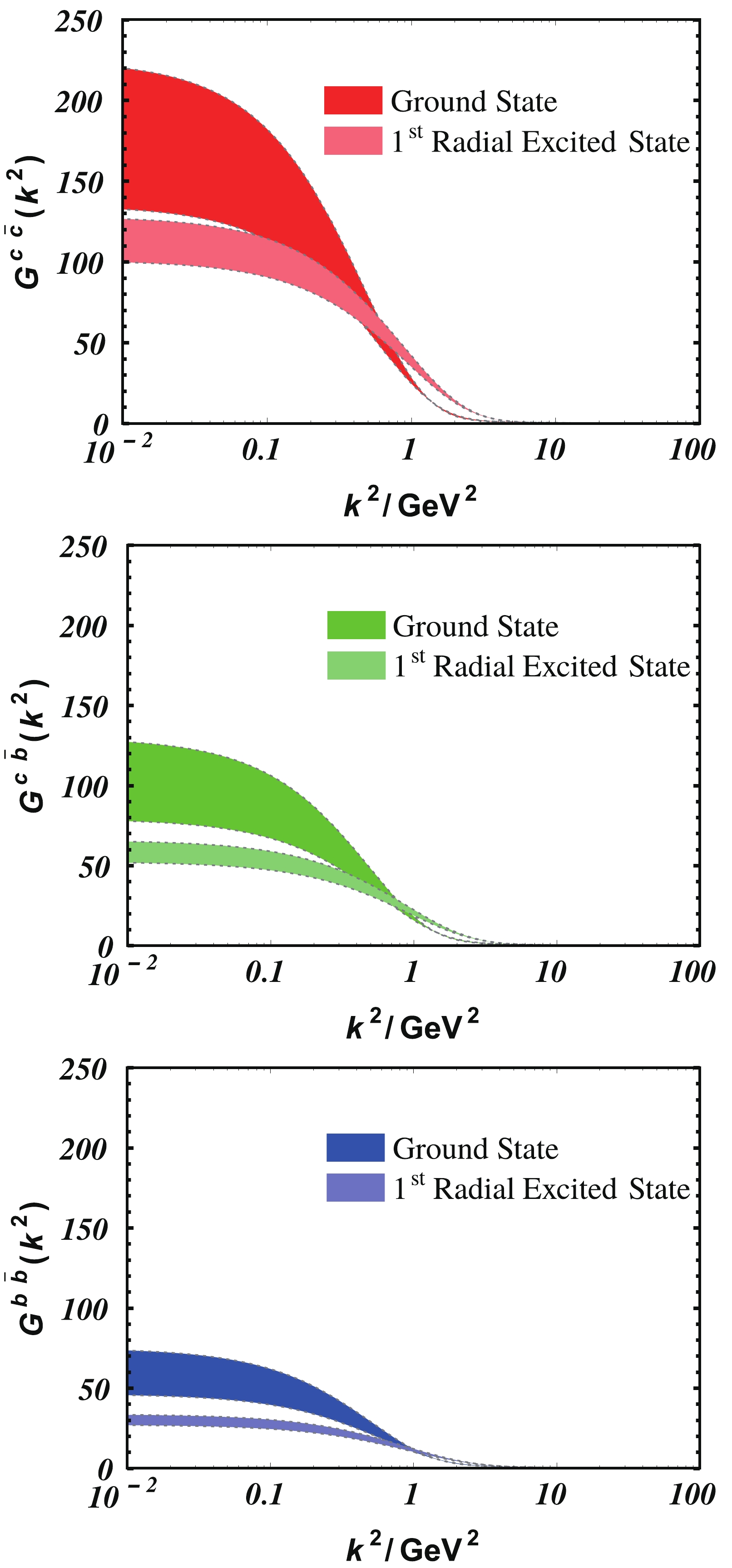
Figure 2. (color online) Effective interaction dressing functions of the ground states (Eqs. (7)-(9)) and the first radial excited states (Eq. (7), Eq.(10) and Eq. (9)). The region boundary is defined by Parameter-1 and Parameter-3 in Table A1 in the appendix.
-
In summary, the first radial excited heavy pseudoscalar and vector mesons (
$ \eta_c(2S) $ ,$ \psi(2S) $ ,$ B_c(2S) $ ,$ B^*_c(2S) $ ,$ \eta_b(2S) $ ,$ \varUpsilon(2S) $ ) are studied with the Dyson-Schwinger equation and the Bethe-Salpeter equation approach. The interaction is refixed by fitting the masses and leptonic decay constants of$ \psi(2S) $ and$ \varUpsilon(2S) $ to the exprimental values. With the interaction well determined, a precise prediction of the masses and leptonic decay constants of$ \eta_c(2S) $ ,$ B_c(2S) $ ,$ B^*_c(2S) $ , and$ \eta_b(2S) $ can be given. This study also shows that, compared with the ground states, the soft part of the effective interaction in the excited states declines and the hard part increases. -
The three groups of parameters corresponding to
$ \omega_u = 0.45, 0.50, 0.55 \;{\rm{ GeV}} $ are listed in Table A1. The quark mass$ \bar{m}_f^{\zeta} $ is defined byflavor $\bar{m}_f^{\zeta=2{\text{GeV}}}$ 

Parameter-1 $w_f $ 

$D_f^2$ 

$\alpha_f$ 

$\eta_f$ 

c 1.17 0.690 0.645 1.360 0.755 b 4.97 0.722 0.258 1.323 0.671 flavor $\bar{m}_f^{\zeta=2{\text{GeV}}}$ 

Parameter-2 $w_f $ 

$D_f^2$ 

$\alpha_f$ 

$\eta_f$ 

c 1.17 0.730 0.599 1.304 0.817 b 4.97 0.766 0.241 1.265 0.730 flavor $\bar{m}_f^{\zeta=2{\text{GeV}}}$ 

Parameter-3 $w_f $ 

$D_f^2$ 

$\alpha_f$ 

$\eta_f$ 

c 1.17 0.760 0.570 1.265 0.865 b 4.97 0.792 0.231 1.225 0.766 Table A1. Three groups of parameters correspond to
$\omega_{u/d} = 0.45, 0.50, 0.55 \;{\text{GeV}}$ .$\bar{m}_f^{\zeta=2{\text{GeV}}}$ ,$\omega_f$ and$D_f$ are measured in GeV. α and η are of unit 1.$\tag{A1} \bar{m}_f^{\zeta} = \hat{m}_f\Big /\left[\frac{1}{2}{\rm{ln}}\frac{\zeta^2}{\Lambda^2_{\rm{QCD}}}\right]^{\gamma_m}, $

$\tag{A2} {\hat m_f} = \mathop {\lim }\limits_{{p^2} \to \infty } {\left[ {\frac{1}{2}{\rm{ln}}\frac{{{p^2}}}{{\Lambda _{{\rm{QCD}}}^2}}} \right]^{{\gamma _m}}}{M_f}({p^2}), $

with ζ being the renormalisation scale,
$ \hat{m}_f $ the renormalisation-group invariant current-quark mass, and$ M_f(p^2) $ the quark mass function.
Radial excited heavy mesons
- Received Date: 2021-08-24
- Available Online: 2021-12-15
Abstract: In this study, the first radial excited heavy pseudoscalar and vector mesons (


 DownLoad: