


 Abstract
 HTML
HTML Reference
 Related
 PDF
PDF


-
It is well known that the gluon density inside a hadron has a rapid growth as the energy increases or the Bjorken-x decreases. Eventually, a new state of high density gluonic matter is expected to be formed. At high gluon density, the non-linear effect becomes important and controls the growth of the gluon density, leading to a saturation state called the color glass condensate (CGC) [1].
The saturation picture of the CGC has been studied over the last two decades. One of the key predictions, the geometric scaling, made by the CGC theory was observed by the deep inelastic scattering (DIS) experiments at HERA [2, 3]. In addition, the charged hadron transverse momentum and multiplicity distributions in deutron-gold (d-Au), proton-lead (p-Pb), and lead-lead (Pb-Pb) collisions at RHIC and LHC energies are also successfully described by the CGC theory [4-6]. The CGC mechanism appears to exhibit a dominant effect on governing the evolution of the partonic system, especially in the early stage of the collisions. However, it was determined that the DGLAP evolution can also provide the geometric scaling [7], while the quantum chromodynamics (QCD) factorization formulation can describe the hadron transverse momentum distribution in high energy heavy ion collisions with equal quality. It is difficult to distinguish the mechanism between the CGC and DGLAP.
It has been determined that the exclusive vector meson production process is sensitive to the saturation physics [8-12]. To test the saturation picture of the CGC and obtain more evidence to support the CGC mechanism, we study the
${J}/\mathrm{\psi} $ production at HERA. Currently, studies on the$ {J}/\mathrm{\psi} $ production within the CGC framework are mainly focused on the leading order (LO) dipole amplitude, resulting from the Balitsky-Kovchegove (BK) evolution equation, which is evolved in terms of the rapidity of the dilute projectile [13, 14]. The LO saturation models, such as the Golec-Biernat and Wusthoff (GBW) [3] and Iancu, Itakura, and Munier (IIM) models [15], were adopted to investigate the exclusive and dissociative${J}/\mathrm{\psi} $ production. In addition to the LO saturation model, a novel model (called the hotspot model), which considers the quantum fluctuation of the proton structure, was proposed recently by the authors of Refs. [16, 17] and promoted by the authors of Ref. [18], and it was applied to study the dissociative vector meson photoproduction. The structural quantum fluctuation of a proton was treated via the variance of the number of regions of high gluon density (hotspots). It was demonstrated that the accuracy of the promoted hotspot model can still be improved [18]. To improve the precision of the hotspot model, it can be deduced that two aspects of the model need to improve. On the one hand, the number of hotspots in this model does not consider the virtuality ($ Q^2 $ ) dependence. As is well known, the functional form of the number of hotspots is inspired by the gluon distribution function, and virtuality is a key factor in the parton distribution function. Therefore, the number of hotspots should include the influence of virtuality. In this study, we extend the hotspot model to consider the virtuality dependence by multiplying a logarithmic factor ($ \ln(Q^2/\Lambda^2) $ ). Our results indicate that the virtuality affects the number of hotspots and improves the capacity of the model in elucidating the experimental data.On the other hand, the dipole amplitudes adopted in the hotspot model are inspired by the LOBK equations [16-18]. It has been determined that these LO dipole amplitudes are insufficient in providing an accurate description of the experimental data at HERA [19]. Furthermore, all the above mentioned dipole amplitudes are expressed in terms of projectile rapidity (Y), because their evolution equations are derived in the Y representation. A recent study determined that a dipole amplitude should be adopted in the target rapidity (
$ \eta $ ) representation to investigate the HERA data, as the data are usually measured in terms of target rapidity, rather than projectile rapidity [20]. The next-to-leading order (NLO) collinear improved Balitsky-Kovchegov evolution equation in the$ \eta $ representation (ciBK-$ \eta $ ) was derived recently and used to investigate the inclusive HERA data [20-22]. It was demonstrated that the ciBK-$ \eta $ can provide a relatively successful description of the proton structure function data [23]. However, the ciBK-$ \eta $ has not confronted the exclusive and dissociative experimental data yet. In this study, the ciBK-$ \eta $ is adopted, for the first time, to realize the exclusive and dissociative vector meson production. This indicates that our proposed method can provide a relatively optimal description of the$ {J}/\mathrm{\psi} $ production HERA data with$ \chi^2/d.o.f = 1.0183 $ for the fit to the total cross section. Our results can provide a significant implication of signature for the CGC at HERA. -
To introduce notations and elucidate the kinematics, we review the
$ {J}/\mathrm{\psi} $ production in this section. The corresponding amplitudes of the$ {J}/\mathrm{\psi} $ production are adopted for comparisons with the experimental data in Sec. IV. -
It is well known that the exclusive and dissociative
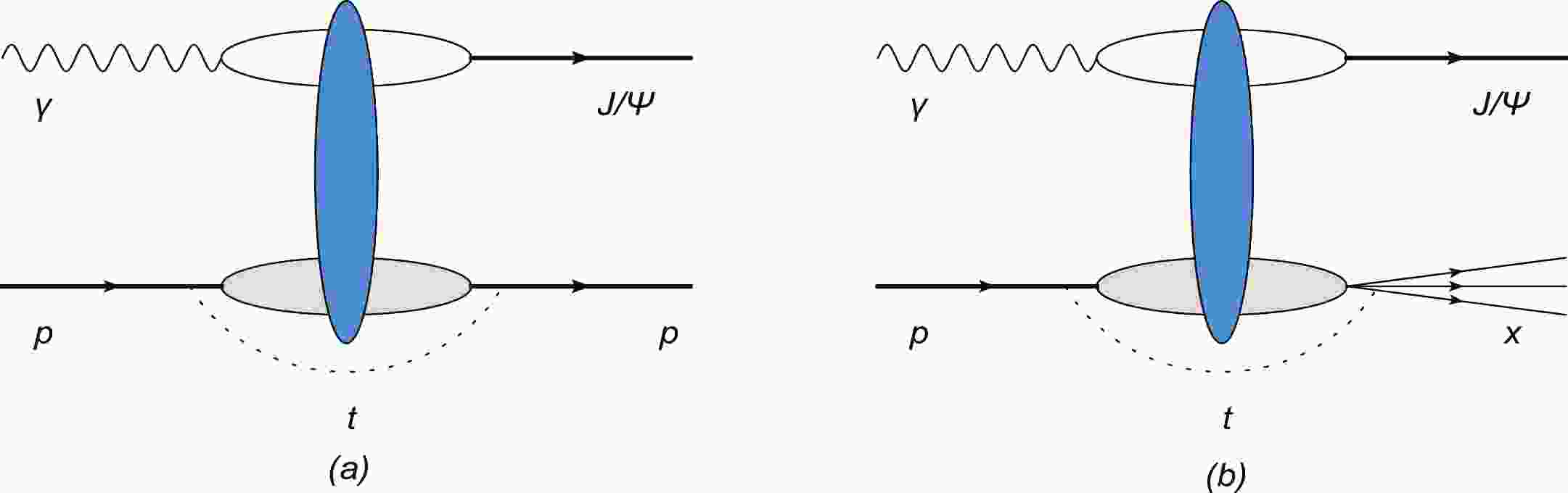
$ {J}/\mathrm{\psi} $ production can be described by the color dipole model [24-26]. In the dipole model, the diffractive meson production process can be divided into three subprocesses. In the first process, an electron emits a virtual photon, and then, the virtual photon fluctuates into a dipole that comprises a quark and antiquark pair. In the second process, the dipole interacts with a target proton by exchanging gluons. Finally, the quark and antiquark are recombined to produce a vector meson, as illustrated in Fig. 1. The vector meson production amplitude can be written as in [16, 27]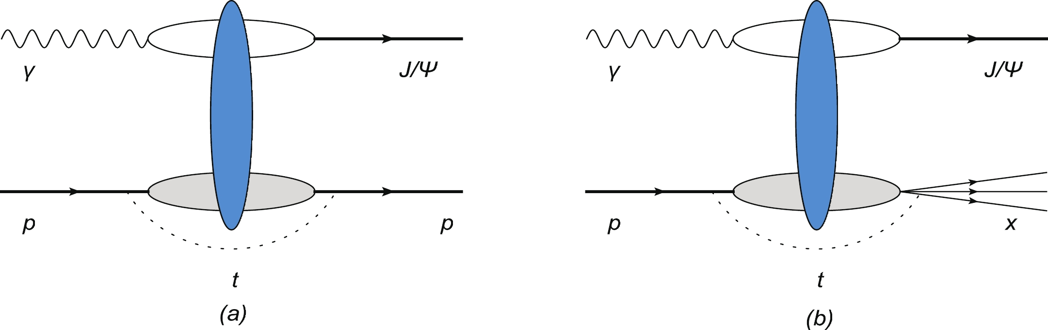
Figure 1. (color online) Diagrams for exclusive (a) and dissociative (b) vector meson productions in dipole-proton scattering.
$ \begin{aligned}[b] A(x,Q^2,\mathbf{\Delta} )_{T,L} =& {\rm i}\int {\rm d}{r}\int_{0}^{1} \frac{{\rm d}z}{4\pi}({\psi^*_V\psi})_{T,L}\\&\times\int {\rm d}{b}{\rm e}^{-{\rm i}({b}-\frac{(1-2z)}{2}{r})\cdot\bf{\Delta}}\frac{{\rm d}\sigma_{\rm dip}}{{\rm d}{b}}, \end{aligned}$

(1) where t = -
$ \mathbf{\Delta}^{2} $ and$ {b} $ represent the squared momentum transfer and the impact parameter between the dipole and proton, respectively. The z in Eq. (1) represents the longitudinal momentum fraction carried by a quark, whose integral ranges from 0 to 1. In addition,$ {r} $ ,$ Q^{2} $ , T, L, and x represent the transverse size of the dipole, photon virtuality, transversely polarized photon, longitudinally polarized photon [17], and Bjorken variable [28], respectively.$ {\psi^*_V\psi} $ represents the overlap wave function of the vector meson and photon, which will be comprehensively discussed later in this section. It should be noted that an exponential phase factor$ \exp\big[-{\rm i}(1-2z){r}\cdot\mathbf{\Delta}/2\big] $ is introduced to Eq. (1) to include the non-forward contribution ($ \mathbf{\Delta}\neq 0) $ . This factor, proposed in Ref. [29], is an improvement of the BGBP factor [30]. It has been determined that the$ \exp\big[-{\rm i}(1-2z){r}\cdot\mathbf{\Delta}/2\big] $ plays a significant role in longitudinally polarized virtual photon process. Therefore, we adopt$ \exp\big[-{\rm i}(1-2z){r}\cdot\mathbf{\Delta}/2\big] $ as the phase factor in this study.The dipole cross-section in Eq. (1) is a key component because it includes most of the scattering information. In terms of optical theorem, it can be expressed as
$ \frac{{\rm d}\sigma_{\rm dip}}{{\rm d}{b}} = 2N(x,{r},{b}), $

(2) where
$ N(x,{r},{b}) $ is the imaginary part of the dipole-target scattering amplitude. To simplify the calculation, we assume that the impact parameter can be factorized out of the dipole amplitude as [18]$ N(x,{r},{b}) = \sigma_{0}N(x,r)\ T ({b}), $

(3) where
$ \sigma_{0} $ is equal to$ 2\pi R_p $ with$ R_p $ being the radius of proton, and$ T({b}) $ is the profile of proton. We would like to point out that the impact parameter$ {b} $ and the momentum transfer$ \mathbf{\Delta} $ are Fourier conjugate variables. The scattering amplitude$ N(x,{r},{b}) $ in$ {b} $ space can be obtained via the Fourier transform of the amplitude$ N(x,{r},{\Delta}) $ in momentum space [31]. Moreover, it is known that the$ \mathbf{\Delta}\neq 0 $ corresponds to non-forward scattering. Therefore, it can be observed that the dipole scattering amplitude in$ {b} $ space include the non-forward information. When we factorize the scattering amplitude into three parts as shown in Eq. (3), the non-forward information is assumed to be included in the$ {b} $ dependent factor$ T({b}) $ .It is known that the proton is a quantum object, and the structure of the proton fluctuates from event to event in the interaction. Based on the hotspot model, all fluctuations are encoded in the proton profile
$ T({b}) $ [16-18]. The proton profile can be defined as the sum of$ N_{hs} $ regions of the hotspots [18]$ T({b}) = \frac{1}{\ N_{hs}}\sum\limits_{i = 1}^{ N_{hs}} T_{hs}({b}-{b}_{i}), $

(4) with
$ T_{hs}({b}-{b}_{i}) = \frac{1}{2\pi B_{hs}}{\rm e}^{\textstyle-\frac{({b}-{b}_{i})^2}{2 B_{hs}}}, $

(5) where
$ {b}_i $ is the location of the$ i^{\rm th} $ hotspot and is assumed to satisfy the two-dimensional Gaussian distribution centered at the origin with a width$ B_p $ . Here,$ B_p $ denotes half the average of the squared transverse radius of the proton, and$ B_{hs} $ represents half the average of the squared transverse radius of the hotspots.The
$ N_{hs} $ in Eq. (4) denotes the number of hotspots and can be expressed as$ N_{hs}(x) = p_{0}x^{p_{1}}(1+p_{2} \sqrt{x})\Big[\ln\Big(\frac{Q^2}{\Lambda^2}\Big)\Big]^{p_{3}}, $

(6) with
$ \Lambda = 0.2\; \mathrm{GeV} $ .$ p_{0} $ ,$ p_{1} $ ,$ p_{2} $ , and$ p_{3} $ are free parameters, which we will determined by fitting to the HERA data in Sec. IV. Note that the functional form of Eq. (6) is inspired by the gluon distribution function [32, 33]. Originally, the number of hotspots defined in Ref. [18] solely includes the Bjorken-x (or energy) information. In fact, the number of hotspots should include both energy and virtuality dependence in terms of the parton distribution function. To promote the hotspot model, as accurate as possible, we include the virtuality dependence into the functional form of the number of hotspots, which is inspired by Ref. [33]. We determine that virtuality plays a significant role in describing the exclusive and dissociative$ {J}/\mathrm{\psi} $ production data at HERA.To simplify the computation, we can rewrite Eq. (1) in terms of the polar coordinate expression
$ \begin{aligned}[b] A (x,Q^2,\mathbf{\Delta} )_{T,L} =& {\rm i}\int r{\rm d}r\int_{0}^{2\pi}{\rm d}{\theta}{\rm e}^{\textstyle -{\rm i}r\frac{(1-2z)}{2}\Delta\cos\theta}\\&\times\int_{0}^{1} \frac{{\rm d}z}{4\pi}({\psi^*_V\psi})_{T,L}\int {\rm d}{b}{\rm e}^{-{\rm i}{b}\cdot{\Delta}}\frac{{\rm d}\sigma_{\rm dip}}{{\rm d}{b}}. \end{aligned}$

(7) By substituting Eqs. (2) and (3) into Eq. (7), the expression of the imaginary part of the scattering amplitude used in the exclusive and dissociative
$ {J}/\mathrm{\psi} $ production can be obtained as$ \begin{aligned}[b] A(x,Q^2,\mathbf{\Delta} )_{T,L} =& {\rm i}\int r{\rm d}r\ N(x,r)\int {\rm d}z ({\psi^*_V\psi})_{T,L} \\&\times J_{0}\left(r\frac{(1-2z)}{2}\Delta\right)\int {\rm d}{b}{\rm e}^{-{\rm i}{b}\cdot{\Delta}} T({b}), \end{aligned}$

(8) where
$ J_0 $ is the first kind Bessel function.In the diffractive exclusive
$ {J}/\mathrm{\psi} $ production, the proton remains intact after the interaction between the dipole and the target, which can be noted by$ \gamma^{*} p \to Vp $ , with the vector meson V ($ {J}/\mathrm{\psi} $ ). Using the scattering amplitude in Eq. (8), the differential scattering cross section of the exclusive vector meson V production is given by [27]$ \frac{{{\rm d}\sigma}^{\gamma^{*} p\to V p}_{T,L}}{{\rm d}t} = \frac{1}{16\pi}\left| \left \langle A(x,Q^2,{\mathbf{\Delta}} )_{T,L} \right \rangle\right|^{2}, $

(9) where the notation
$ \left \langle \right \rangle $ represents the average over the target configuration.For the dissociative
${J}/\mathrm{\psi} $ production, the proton dissociates into a new system. This process can be expressed as$ \gamma^{*} p\to V X $ , where X is the dissociation state of the proton. The dissociative differential scattering cross section of V production can be written as [17]$ \begin{aligned}[b] \frac{{{\rm d}\sigma}^{\gamma^{*} p\to V X}_{T,L}}{{\rm d}t} =& \frac{1}{16\pi}\left( \left \langle \left| A(x,Q^2,\mathbf{\Delta} )_{T,L} \right|^{2} \right \rangle\right.\\&\left.-\left| \left \langle A(x,Q^2,\mathbf{\Delta} )_{T,L} \right \rangle\right|^{2}\right), \end{aligned} $

(10) the Bjorken variable x is given by
$ x = (\ M_{V}^{2}+Q^2)/(\ W_{\gamma^{*} p}^2 +Q^2), $

(11) where
$ M_V $ and$ W_{\gamma^{*} p} $ denote the mass of vector meson and the center of mass energy, respectively. -
Regarding the overlap function in Eq. (1), there are several types in the literature. It seems that a vector meson has its own specific favorite overlap function [31]. However, we focus on studying the higher order corrections of the dipole amplitude in this study and attempt to solely the boosted Gaussian model [34, 35], as this model can describe both light and heavy mesons, simultaneously [36]. The overlap functions are written as [27]
$ \begin{aligned}[b] ({\psi^*_{V}\psi})_T =& \hat{e}_fe{\frac{N_c}{{\pi}z(1-z)}}\Big\{ m^2_f K_0(\epsilon r) \phi_T(r,z)\\&-\big [{z^2}+(1-z)^2 \big ]{\epsilon }K_1({\epsilon } r)\partial_r\phi_T(r,z)\Big\},\end{aligned} $

(12) $ \begin{aligned}[b] ({\psi^*_V\psi})_L =& \hat{e}_fe{\frac{N_c}{\pi}}2Qz(1-z)K_0(\epsilon r)\\&\times\Big [M_V\phi_L(r,z)+\delta{\frac{m^2_f-\nabla^2_r}{M_Vz(1-z)}}\phi_L(r,z) \Big ], \end{aligned}$

(13) where
$ K_{0}(\epsilon r) $ and$ K_{1}({\epsilon } r) $ are the second kind bessel functions, and$ \epsilon $ is a variable defined by$ \epsilon ^2 = z(1-z)Q^2 +m_f^2 $ with$ m_{f} $ as the mass of the quark.$ \psi $ is a wave function used to describe the splitting of the virtual photon into the quark and antiquark, which can be calculated by QED [16, 17]. The$ \psi^*_V $ is the vector meson wave function, which describes the probability of a quark and antiquark pair recombining into a final vector meson [17]. In the above two equations, the parameter$ \delta $ is set to 1,$ N_c = 3 $ is the QCD color number,$ e = \sqrt{4\pi\alpha_{em}} $ is a unit charge, and$ \hat{e}_f $ is the charge of a quark.$ \phi_{T}(r,z) $ and$ \phi_{L}(r,z) $ represent the transverse and longitudinal scalar parts of the vector meson wave function, respectively, which are given by$ \begin{aligned}[b] \boldsymbol{\phi}_{T,L}(r,z) = &N_{T,L}z(1-z)\exp\Bigg (-\frac{ m_{f}^{2} R^{2}}{8z(1-z)}\\&-\frac{2z(1-z) r^{2}}{R^{2}}+\frac{ m_{f}^{2} R^{2}}{2}\Bigg ), \end{aligned} $

(14) the specific parameter values of
$ M_V $ ,$ m_f $ ,$ N_{T,L} $ ,$ R^2 $ and$ \hat{e}_f $ are presented in Table 1.Meson $ \ M_{V}/\mathrm{GeV} $ 

$ \ m_{f}/\mathrm{GeV} $ 

$ \ N_{T} $ 

$ \ N_{L} $ 

$ \ R^{2}/ \mathrm{GeV}^{-2} $ 

$ \hat{e}_f $ 

${J}/\mathrm{\Psi}$ 

3.097 1.4 0.578 0.575 2.3 2/3 Table 1. The parameters of the scalar wave function of
$ {J}/\mathrm{\Psi} $ production in the boosted Gaussian model [27].We would like to note that the longitudinal contribution of the wave function is usually ignored owing to its negligible contribution at a lower
$ Q^2 $ value [12]. In Fig. 2, we present the transverse and longitudinal distributions of overlapping wave functions for$ {J}/\mathrm{\psi} $ at different$ Q^2 $ . From Fig. 2, one can find that the contribution of the longitudinal wave function is also significant at larger$ Q^2 $ . Therefore, the longitudinal contribution of the wave function will be included in our study.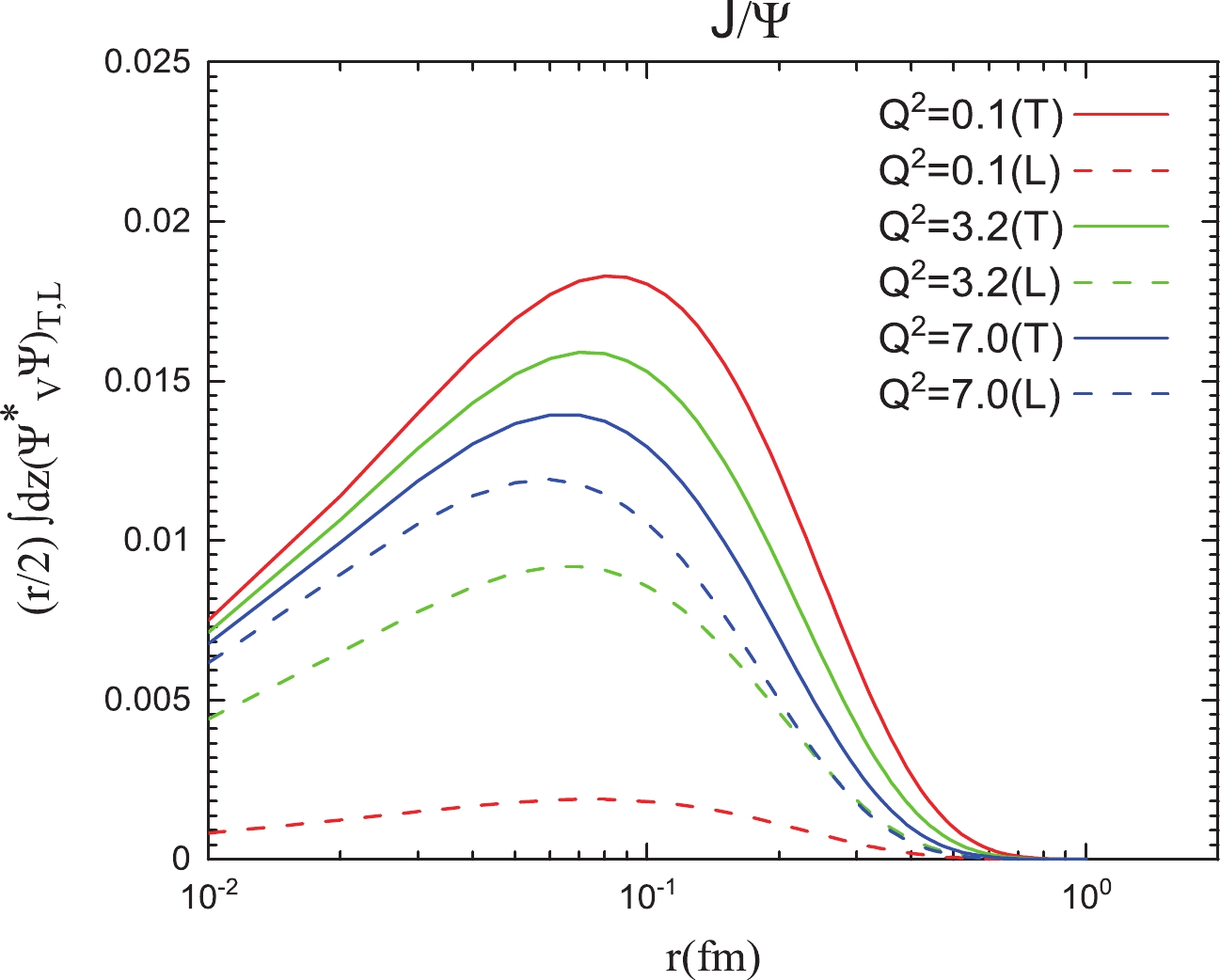
Figure 2. (color online) Comparing the transverse and longitudinal overlap wave functions of
$ {J}/\mathrm{\psi} $ at different$ Q^2 $ . The solid and dashed lines denote the transverse and longitudinal wave functions of$ {J}/\mathrm{\psi} $ , respectively. -
The dipole scattering amplitude plays a key role in calculating the cross sections of the exclusive and dissociative vector meson production, as it encodes all the scattering information between the dipole and target. According to the literature, there are two methods for obtaining the dipole amplitude. In the LO case, the modeling of the dipole amplitude is adopted, such as GBW [3] and IIM [15], which is inspired by the analytic solution of the LOBK equation. The other approach to obtaining the dipole amplitude is to solve its evolution equation numerically. The latter method is conventionally employed in the NLO case. In this study, we adopt the numerical method to uniformly calculate the LO and NLO dipole amplitudes. First, we introduce the evolution equations of the dipole amplitude. Then, we solve them numerically.
-
In the high energy dipole-target scattering, we assume that a dipole consisting of a quark leg at the transverse coordinate
$ {x} $ and an antiquark leg at transverse coordinate$ {y} $ , with a target, moves along the positive and negative directions of the z-axis, respectively. In the LO case, we work within the dipole framework in which all the rapidities are carried by the dipole, and the target is fixed; hence, it is possible for the$ q \bar{q} $ dipole to emit a gluon. Under the limit of a large$ N_c $ , the probability of the quark-antiquark-gluon state production can be calculated [25, 37]. The probability of this new state during scattering is$ \ {\rm d} P = \frac{\alpha N_{c} }{2\pi^2} {\rm d}^{2} {z} {\rm d}Y \frac{({x}-{y})^{2}}{({x}-{z})^{2}({z}-{y})^{2}}, $

(15) where Y represents the rapidity of the projectile.
$ {x} $ and$ {y} $ denote the transverse coordinates of quark and antiquark, respectively.$ {x}-{y} $ is the transverse size of the parent$ q \bar{q} $ dipole, and$ {z} $ stands for the transverse coordinate of the emitted gluon. In Eq. (15),$ {x}-{z} $ and$ {z}-{y} $ represent the transverse size of two new dipoles. The S matrix will change as the rapidity changes, and it is expressed as$ \begin{aligned}[b] \frac{\partial S({x}-{y},Y)}{\partial Y} =& \frac{\alpha N_{c} }{2\pi^2} \int {\rm d}^{2} {z} \frac{({x}-{y})^{2}}{({x}-{z})^{2}({z}-{y})^{2}}\\& \times \Big[{S^{(2)}({x}-{z},{z}-{y},Y)}-S({x}-{y},Y)\Big], \end{aligned}$

(16) among them,
$ S^{(2)}({x}-{z},{z}-{y},Y) $ and$ S({x}-{y},Y) $ denote the scattering amplitudes of two new dipoles interacting with the target and a single dipole interacting with the target, respectively. Under the mean field approximation [38, 39],$ {S^{(2)}({x}-{z},{z}-{y},Y)} = S({x}-{z},Y)S({z}-{y},Y). $

(17) By substituting Eq. (17) into Eq. (16), a closed evolution equation can be obtained as
$ \begin{aligned}[b] \frac{\partial S({x}-{y},Y)}{\partial Y} =& \frac{\alpha N_{c} }{2\pi^2} \int {\rm d}^{2} {z} \frac{({x}-{y})^{2}}{({x}-{z})^{2}({z}-{y})^{2}}\\& \times\Big[S({x}-{z},Y)S({z}-{y},Y)-S({x}-{y},Y)\Big], \end{aligned} $

(18) which is known as the BK evolution equation [13, 14]. As is well-know, the relationship between the scattering amplitude and the S matrix is
$ N({x}-{y},Y) = 1-S({x}-{y},Y). $

(19) By substituting Eq. (19) into Eq. (18), we can obtain another form of the BK equation as [14]
$ \begin{aligned}[b] \frac{\partial N({x}-{y},Y)}{\partial Y} =& \int {\rm d}^{2} {z} K^{\rm LO}\Big[N({x}-{z},Y)+N({z}-{y},Y)\\ &-N({x}-{y},Y)-N({x}-{z},Y)N({z}-{y},Y)\Big], \end{aligned} $

(20) where the evolution kernel is
$ \ K^{\rm LO} = \frac{\alpha N_{c} }{2\pi^2} \frac{({x}-{y})^{2}}{({x}-{z})^{2}({z}-{y})^{2}}. $

(21) A nonlinear term
$ N({x}-{z},Y)N({z}-{y},Y) $ exists in Eq. (20), which indicates that two new dipoles interact with the target simultaneously and ensures the unitarity of the scattering amplitude. -
The LOBK equation solely considers the leading logarithmic contribution with fixed
$ \alpha_{s} $ , whereas NLO corrections are ignored. It has been determined that the LOBK equation is insufficient in providing an accurate description of the experimental data HERA [19], which indicates that the NLO corrections are required. The complete NLO BK evolution equation was derived in Ref. [40], where the corrections of quark and gluon loops, as well as tree gluon diagrams with quadratic and cubic nonlinearities, are included. However, the complete NLO BK equation cannot be directly applied to phenomenology because its numerical solution significantly depends on the details of the initial conditions and can turn to negative for small size dipoles [41], which is usually considered an instability problem. It was inferred that the instability issues are related to a large double logarithmic term in the evolution kernel, which leads to a negative dipole amplitude. To address these issues, a novel method was proposed to resum all orders in the radiative corrections enhanced by large double transverse logarithms [42]. A ciBK equation was obtained by including the time ordering constrain in the successive gluon emissions [42].Although the instability problem was temporarily solved by the collinear improved method, all the aforementioned evolution equations were derived in the projectile (dipole) framework, where the projectile rapidity is considered the “evolution time” in the high energy evolution. Based on the previous experience with the NLO BKFL equation [43], the instability of the full NLO BK equation is a consequence of the “wrong choice of evolution variable.” To completely solve the instability problem, the evolution equation in the target framework needs to be re-derived, where the target rapidity is considered “evolution time.” As is known, the target is a nucleus and its wavefunction is saturated for modes softer than the saturation scale. In addition, it is difficult to directly derive the evolution equation in the target frame. Fortunately, an ingenious method was proposed in Ref. [20], where the authors adopt the change in variables to transform the results of the perturbation theory from the Y-representation to the
$ \eta $ -representation,$ Y \; \; \rightarrow \; \; \eta \equiv Y - \rho, $

(22) with
$ \rho = \ln(1/r^2Q_0^2) $ . The various S-matrices can be rewritten as$ S({x}-{y},Y) = S({x}-{y},\eta+\rho) \equiv \bar{S}({x}-{y},\eta), $

(23) $ \begin{aligned}[b] S({y}-{z},Y) = & S({y}-{z},\eta+\rho) = S\Bigg({y}-{z},\eta+\rho_{{y}{z}}\\&+\ln\frac{({y}-{z})^2}{({x}-{y})^2}\Bigg) \equiv \bar{S}\Bigg({y}-{z},\eta+\ln\frac{({y}-{z})^2}{({x}-{y})^2}\Bigg) \end{aligned} $

(24) and
$ \begin{aligned}[b] S({z}-{x},Y) =& S({z}-{x},\eta+\rho) = S\Bigg({z}-{x},\eta+\rho_{{z}{x}}\\&+\ln\frac{({z}-{x})^2}{({x}-{y})^2}\Bigg) \equiv \bar{S}\Bigg({z}-{x},\eta+\ln\frac{({z}-{x})^2}{({x}-{y})^2}\Bigg). \end{aligned} $

(25) Upon substituting the above three equations into Eq. (18), Eqs. (24) and (25) need to be expanded, and the first non-trivial term must be maintained in the expansions:
$ \begin{aligned}[b] \bar{S}\Bigg({y}-{z},\eta+\ln\frac{({y}-{z})^2}{({x}-{y})^2}\Bigg) \simeq & \bar{S}({y}-{z},\eta) + \ln\frac{({y}-{z})^2}{({x}-{y})^2}\frac{\partial \bar{S}({y}-{z},\eta)}{\partial \eta} = \bar{S}({y}-{z},\eta) + \frac{\bar{\alpha}_s}{2\pi}\int {\rm d}^2{u}\frac{({y}-{z})^2}{({y}-{u})^2({u}-{z})^2} \ln\frac{({y}-{z})^2}{({x}-{y})^2} \\ & \times\big[\bar{S}({y}-{u},\eta)\bar{S}({u}-{z},\eta)-\bar{S}({y}-{z},\eta)\big], \end{aligned} $ 
(26) and
$ \begin{aligned}[b] \bar{S}\Bigg({z}-{x},\eta+\ln\frac{({z}-{x})^2}{({x}-{y})^2}\Bigg) \simeq& \bar{S}({z}-{x},\eta) + \ln\frac{({z}-{x})^2}{({x}-{y})^2}\frac{\partial \bar{S}({z}-{x},\eta)}{\partial \eta} = \bar{S}({z}-{x},\eta) + \frac{\bar{\alpha}_s}{2\pi}\int {\rm d}^2{u}\frac{({z}-{x})^2}{({z}-{u})^2({u}-{x})^2}\ln\frac{({z}-{x})^2}{({x}-{y})^2} \\ & \times\big[\bar{S}({z}-{u},\eta)\bar{S}({u}-{x},\eta)-\bar{S}({z}-{x},\eta)\big]. \end{aligned} $

(27) By substituting Eqs. (23), (26), and (27) into Eq. (18), and applying the time ordering condition, the ciBK equation can be obtained in the
$ \eta $ representation (ciBK-$ \eta $ ) as [20]$ \begin{aligned}[b] \frac{\partial\bar{N}({x}-{y},\eta)}{\partial \eta} =& \frac{\bar{\alpha}_s}{2\pi}\int {\rm d}^2{z} \frac{({x}-{y})^2}{({y}-{z})^2({z}-{x})^2} \bigg[\bar{N}({y}-{z},\eta-\delta({y}-{z},{x}-{y})) + \bar{N}({z}-{x},\eta-\delta({z}-{x},{x}-{y})) - {\bar{N}}({x}-{y},\eta) \\ &-\bar{N}({y}-{z},\eta-\delta({y}-{z},{x}-{y}))\bar{N}({z}-{x},\eta-\delta({z}-{x},{x}-{y})) \bigg] , \end{aligned} $

(28) where
$ \bar{N} = 1-\bar{S} $ is adopted, and the rapidity shifts are$ \delta({y}-{z},{x}-{y})\equiv \mathrm{max}\Bigg\{0,\ln\frac{({x}-{y})^2}{({y}-{z})^2}\Bigg\}, $

(29) and
$ \delta({z}-{x},{x}-{y})\equiv \mathrm{max}\Bigg\{0,\ln\frac{({x}-{y})^2}{({z}-{x})^2}\Bigg\}. $

(30) Note that Eq. (28) can be used to describe the DIS data without any assumptions, as the rapidity
$ \eta $ of the hadronic target is directly adopted in the DIS measurements. If an evolution equation in the Y representation is adopted, it is necessary to either transfer the results from the Y representation to the$ \eta $ representation or blindly assume Y to be as$ \eta $ when fit to the HERA data. However, it is difficult to draw a firm conclusion from the latter. -
From the LOBK expressions and ciBK-
$ \eta $ equations introduced in Secs. III A and III B, it can be observed that they all belong to integro-differential equations. In this section, we first discretize the size of the dipole and then numerically solve the above mentioned two equations on the lattice. We adopt the GNU science library (GSL) to carry out the numerical simulation, because GSL can provide adaptive integral subroutines to perform the integrations, and the Runge-Kutta method in the GSL can be used to solve the differential equations on the lattice [22, 44]. Simultaneously, to obtain the data points that are not located on the lattice, the cubic spline interpolation method is adopted.To solve the differential equations, we adopt the GBW model as the initial condition [3]. To elucidate the difference between the LOBK and ciBK-
$ \eta $ equations, we plot the solutions of the LOBK and ciBK-$ \eta $ equations (dipole amplitudes) as a function of the dipole sizes r for three different target rapidities in Fig. 3. From Fig. 3, it can be inferred that the LO and ci dipole amplitudes are close to each other when the rapidities are small. As the rapidity increases, it can be observed that the LO dipole amplitudes are always larger than the ones with the higher order radiative corrections. In Fig. 3, it can be observed that the evolution of the LO dipole amplitude is very rapid, while the evolution speed of the ci dipole amplitude is inhibited by higher order corrections, which indicates that the collinear improved effect significantly contributes to suppressing the evolution of the dipole amplitude [42]. In the next section, it can be inferred that the improvements in the description of the HERA data are precisely owing to the already mentioned suppression effect.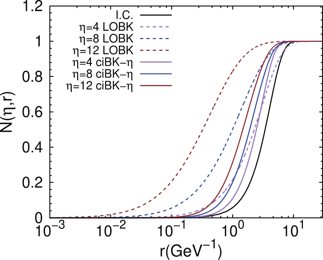
Figure 3. (color online) Numerical solutions to the LOBK and ciBK-
$ \eta $ equations for three different target rapidities. -
In this section, we use the formula introduced in previous two sections to fit the
${J}/\mathrm{\psi} $ experimental data. The data are obtained from ZEUS [45] and H1 [46] collaborations. Because we are focusing on the small-x physics in this study, the data with$ x>0.01 $ are excluded. Moreover, we only consider the data with$ 1<Q^2<60\; \mathrm{GeV}^2 $ . The lower limit on$ Q^2 $ is selected to ensure that work is performed in the perturbative region. The upper limit on$ Q^2 $ is set large enough to include as much as possible “perturbative” data points but low enough to validate the use of small-x dynamics, rather than DGLAP dynamics.It should be noted that the number of hot spots in Eq. (6) is introduced by the inspiration of the
$ Q^2 $ dependent gluon distribution function. As$ Q^2 $ sets the resolution scale in the transverse plane,$ Q^2 $ will affect both the number and the size of hotspots. To explore these effects, we shall carry out the fit by using Eq. (6) with a series values of$ B_{hs} $ , which vary from 0.7 to 0.82$ \; \mathrm{GeV}^{-2} $ , as presented in Tables 2 and 3. The relevant parameters presented in Tables 2 and 3 correspond to the fit of the total cross sections with the dipole amplitude from the ciBK-$ \eta $ and LOBK equations, respectively. We obtain the best quality of fit at$ B_{hs} = 0.76\; \mathrm{GeV}^{-2} $ in both ciBK-$ \eta$ and LOBK cases, and the$ \chi^2/d.o.f $ becomes worse when the$ B_{hs} $ shifts to either small or large values. This value is smaller than that one$ (B_{hs} = 0.8\; \mathrm{GeV}^{-2}) $ obtained by the$ Q^2 $ independent hotspot model in Ref. [18], which indicates that the size of hotspots decreases when the$ Q^2 $ values are considered in the hotspot model. In addition, the$ p_3 $ parameter in Eq. (6), which reflects the dependence of the number of hotspots on$ Q^2 $ , increases as$ B_{hs} $ decreases. This result indicates that the$ Q^2 $ has a significant impact on the number and the size of hotspots. From Tables 2 and 3, it can be observed that the values of$ \chi^2/d.o.f $ (1.0183) resulting from ciBK-$ \eta$ equation are more approximate to the unit than the corresponding ones (1.3995) originating from LOBK equation. These results indicate that the collinear improved BK equation in the$\eta$ representation provides a better description of the HERA data than the LOBK equation. We would like to point out that we adopted an improved phase factor to include the non-forward contribution in Eq. (1). We also carried out the fit by using the phase factor proposed in Ref. [30] with collinear improved dipole amplitude. This gives a relatively poor$ \chi^2/d.o.f $ when compared to the improved phase factor, which indicates that the improved phase factor enhances the theoretical description of the data.$B_{hs}/\mathrm{GeV}^{-2}$ 

$ \chi^2 $ /

$ d.o.f $ 

$ p_{0} $ 

$ p_{1} $ 

$ p_{2} $ 

$ p_{3} $ 

0.7 1.2946 0.0062 −0.5451 423.4428 0.1432 0.73 1.1736 0.0058 −0.5456 455.8736 0.1357 0.76 1.0183 0.0059 −0.5443 451.0784 0.1320 0.79 1.1354 0.0065 −0.5430 409.6127 0.1315 0.82 1.2523 0.0073 −0.5201 421.5528 0.1245 Table 2. Parmeters and
$ \chi^2 $ /$ d.o.f $ from the fit to total cross section of$ J/\Psi $ production with the dipole amplitude from the ciBK-$\eta$ equation.$B_{hs}/\mathrm{GeV}^{-2}$ 

$\chi^2$ /

$d.o.f$ 

$p_{0}$ 

$p_{1}$ 

$p_{2}$ 

$p_{3}$ 

0.7 1.8942 0.0074 −0.5047 404.0211 0.3372 0.73 1.6703 0.0072 −0.5109 402.7923 0.3261 0.76 1.3995 0.0068 −0.5198 401.0062 0.3220 0.79 1.6302 0.0070 −0.5136 406.6679 0.3134 0.82 1.8236 0.0071 −0.5048 423.6126 0.3109 Table 3. Parmeters and
$\chi^2$ /$d.o.f$ from the fit to total cross section of$J/\psi$ production with the dipole amplitude from the LOBK equation.To elucidate the influence of
$ Q^2 $ on the size and number of hot spots, we plot the$ Q^2 $ dependence of the number of hot spots$ N_{hs} $ at different$ B_{hs} $ with parameters fitted from the ciBK-$ \eta $ equation, as presented in Fig. 4. From Fig. 4, it can be observed that the number of hotspots increases as$ Q^2 $ increases, and the number of hotspots increases as$ B_{hs} $ decreases. These results are consistent with the results from Tables 2 and 3.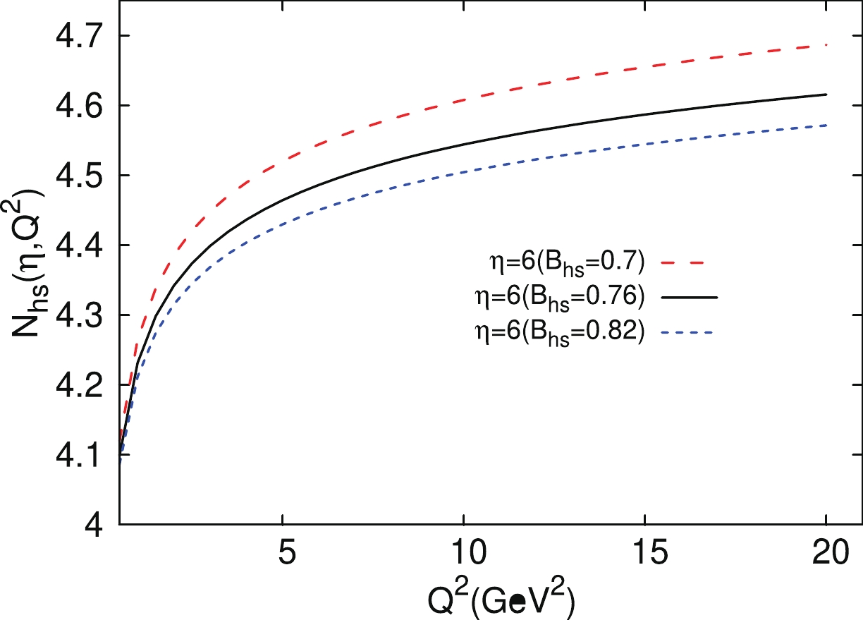
Figure 4. (color online) Number of hotspots as a function of
$ Q^2 $ at different$ B_{hs} $ .The differential cross sections of the exclusive and dissociative
${J}/\mathrm{\psi} $ production for different$ \mathrm{Q}^{2} $ are presented in Fig. 5. The solid squares and circles denote data points from the ZEUS and H1 collaborations hereafter in the following figures, respectively. From the left hand panel of Fig. 5, it can be observed that the theoretical calculations of the differential cross section of exclusive$ {J}/\mathrm{\psi} $ production are almost across all the data points, which indicates that our virtuality improved hotspot model combined with collinear improved dipole amplitude in the$ \eta $ representation provides a relatively optimal description of the HERA data. The right hand panel of Fig. 5 presents the differential cross section of the dissociative$ {J}/\mathrm{\psi} $ production. We cannot determine any experimental measurements of the dissociative$ {J}/\mathrm{\psi} $ production for$ Q^2>1\; \mathrm{GeV}^2 $ . Therefore, we provide an extension of the theoretical calculations at$ Q^2 = 0.1\; \mathrm{GeV}^2 $ , although the data points in our fit have a lower limit on$ Q^2 $ . It seems that the theoretical results (solid lines in the right the hand panel of Fig. 5) are in agreement with the H1 data. In the right hand panel of Fig. 5, the dash-dot, dash, and dot lines depict the theoretical predictions of the differential cross section of the dissociative$ {J}/\mathrm{\psi} $ production at 3.2, 7.0, and 22.4 GeV2 virtualities, respectively.
The total cross sections of the exclusive and dissociative
$ {J}/\mathrm{\psi} $ production for different$ {Q}^{2} $ are presented in Fig. 6. From the left hand panel of the figure, it can be inferred that our virtuality improved hotspot model, combined with the collinear improved dipole scattering amplitude, accurately describes the energy evolution of the exclusive cross section for the available experimental data. We also verify that the original hot spot model present in Ref. [18] with the collinear improved dipole amplitude provides a relatively poor description of the data than our combination. As mentioned above, we also provided an extended theoretical calculations of the total cross section of the dissociative$ {J}/\mathrm{\psi} $ production at$ Q^2 = 0.1\; \mathrm{GeV}^2 $ , as presented in the right hand panel of Fig. 6. Coincidentally, our theoretical results agree well with the measurements. In the right hand panel of Fig. 6, we provide the theoretical predictions of the total cross section of the dissociative$ {J}/\mathrm{\psi} $ production at 3.2 (dash-dot line), 7.0 (dash line), and 22.4 (dot line) GeV2 virtualities, respectively.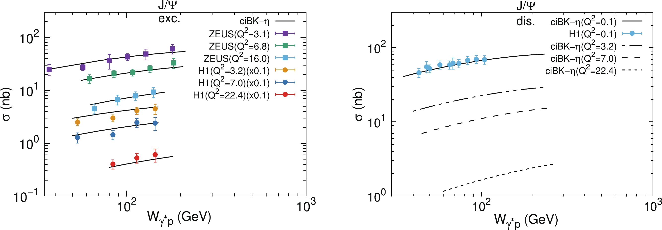
The theoretical calculations of the
$ Q^2 $ distribution of the total cross section of the exclusive and dissociative$ {J}/\mathrm{\psi} $ production are presented in Fig. 7. The left hand panel of Fig. 7 shows that our virtuality improved hotspot model, combined with the collinear improved dipole amplitude in the$ \eta $ representation, can reproduce the measurements relatively successfully. By analyzing the origin of the improvement, the following can be inferred: (i) the virtuality dependence is significant, which takes a slight enhancement of the number of the hotspots; (ii) the LOBK evolution equation overestimates the evolution speed of the dipole amplitude, as the ciBK-$ \eta $ equation provides a dipole amplitude favored by the HERA data; and (iii) the dipole amplitude resulting from the ciBK-$ \eta $ adopts the target rapidity as evolution variable, which is the physical variable directly used in the DIS measurement. This result differs from that of most of studies in literature, where they blindly assumed the projectile rapidity to be the physical rapidity [20, 23]. In the right hand panel of Fig. 7, we preset the predictions of the$ Q^2 $ evolution of the total cross sections of the dissociative$ {J}/\mathrm{\psi} $ production.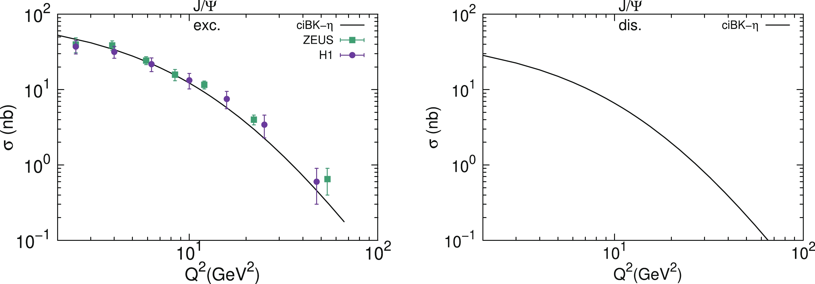
In summary, the exclusive and dissociative
$ {J}/\mathrm{\psi} $ production is studied using a virtuality improved hotspot model combined with a collinear improved dipole amplitude in the$ \eta $ representation at HERA energies. By comparing the theoretical results of the differential and total cross sections calculated from the LOBK and ciBK-$ \eta $ equations with the HERA data, it can be inferred that the dipole amplitude resulting from ciBK-$ \eta $ can provide a more successful description of the experimental data than the LOBK dipole amplitude. The reason for this improvement can be attributed to two main aspects. On the one hand, the evolution speed of the leading order dipole amplitude is too fast to depict the data, and the collinear improved dipole amplitude includes higher order corrections that adopt the suppression of the evolution speed and lead to a successful reproduction of the experimental data. On the other hand, the influence of$ Q^2 $ on the number and size of hotspots are considered. Finally, we would like to emphasize that the significant outcomes of our studies can provide a further implication of the CGC at HERA.
Exclusive and dissociative J/ψ production with collinear-improved Balitsky-Kovchegov equation
- Received Date: 2021-01-09
- Available Online: 2021-07-15
Abstract: We extend the hotspot model to include the virtuality dependence and use it to study the exclusive and dissociative


 DownLoad: