


 Abstract
 HTML
HTML Reference
 Related
 PDF
PDF


-
Topological charge Q and its density
$ q\left(x\right) $ play an important role in the study of the non-trivial topological structure of QCD vacuum. Topological properties have important phenomenological implications, such as$ \theta $ dependence and spontaneous chiral symmetry breaking. The confinement may also be related to nontrivial topological properties [1-3]. The topology of QCD gauge fields is a non-perturbative issue; therefore, the lattice method is a good choice to investigate it from first principles. Lattice QCD is powerful for studying the topological structure of the vacuum. There are many definitions of the topological charge for a lattice gauge field [4-6]. These definitions can be characterized either as gluonic or fermionic. In the fermionic definition, topological charge Q is the number of zero modes of the Dirac operator [7, 8]. In contrast, topological charge can be given by the field strength tensor (gluonic definition) on the lattice, and this definition approaches the fermionic definition in the limit$ a\rightarrow0 $ [9-11].The overlap Dirac operator is a solution of the Ginsparg-Wilson equation [12, 13], and the topological charge defined from the overlap fermion will be an exact integer. In the traditional method, the point source is used in the calculation of topological charge density [14, 15], which makes the computation on the large lattice almost impossible. To reduce the computational cost, the symmetric multi-probing source (SMP) method is introduced to calculate the topological charge density [16]. As the Wilson mass parameter m varies, the value of Q may change [17-20]. The topological charge density
$ q\left(x\right) $ has a strong correlation with the low-lying modes of the Dirac operator, which strongly influences how quarks propagate through the vacuum. Therefore, the topological charge density$ q\left(x\right) $ is a useful probe of the gauge field. We visualize the topological charge density and view the detailed extra information [21]. In contrast, the topological charge cannot show the details of the QCD vacuum. Therefore, we will focus on the topological charge density$ q\left(x\right) $ in the study of the topological properties of the QCD vacuum. We show an analysis of the topological charge$ q\left(x\right) $ , obtained using the fermionic definition with different values of m and the gluonic definition with different Wilson flow time. Unlike in the case of Ref. [22], which studied just one time slice, we consider all time slices and show more details on the topological charge density with different topological charge. By analyzing the topological charge density$ q\left(x\right) $ , we can obtain a great amount of information about the underlying topological structure. We show a comparison with the gluonic topological charge density that is calculated after the application of the Wilson flow method. This comparison is shown by calculating the matching parameter$\Xi_{AB}$ , which is defined later.$\Xi_{AB}$ is used to measure the match of the topological charge density between the fermionic and gluonic definitions. The best match is found when the matching parameter is nearest to$ 1 $ . The proper flow time of Wilson flow in the gluonic definition can also be obtained by analyzing the matching procedure. The behavior of the proper flow time toward the continuum limit is also discussed. -
The pure gauge lattice configurations were generated using a tadpole improved, plaquette plus rectangle gauge action through pseudo-heat-bath algorithm [23, 24]. This gauge action at tree-level
$ \mathcal{O}\left(a^{2}\right) $ -improved is defined as$ S_{G} = \frac{5\beta}{3}\sum\limits_{\textstyle{x\mu\nu\atop \nu>\mu}}{\rm{Re}}{\rm{Tr}}\left[1-P_{\mu\nu}(x)\right]-\frac{\beta}{12u_{0}^{2}}\sum\limits_{\textstyle{x\mu\nu\atop \nu>\mu}}{\rm{Re}}{\rm{Tr}}\left[1-R_{\mu\nu}(x)\right], $

(1) where
$ P_{\mu\nu} $ is the plaquette term. The link product$ R_{\mu\nu}\left(x\right) $ denotes the rectangular$ 1\times2 $ and$ 2\times1 $ loops. The mean link$ u_{0} $ is the tadpole improvement factor that largely corrects for the quantum renormalization of the coefficient for the rectangles relative to the plaquette.$ u_{0} $ is given by$ u_{0} = \left(\frac{1}{3}\text{Re}\thinspace\text{Tr}\langle P_{\mu\nu}\left(x\right)\rangle \right)^{1/4}.$

(2) In the fermionic definitions, we use the overlap operator to calculate topological charge density. The massless overlap Dirac operator is given by [20]
$ D_{\text{ov}} = \left({1}+\frac{D_{\rm{W}}}{\sqrt{D_{\rm{W}}^{\dagger}D_{\rm{W}}}}\right), $

(3) where
$ D_{\rm{W}} $ is the Wilson Dirac operator,$\begin{aligned}[b] D_{{\rm W}} =& \delta_{a,b}\delta_{\alpha,\beta}\delta_{i,j}-\kappa\sum\limits_{\mu = 1}^{4}\Big[\left({1}-\gamma_{\mu}\right)_{\alpha\beta} U_{\mu}\left(i\right)_{ab}\delta_{i,j-\hat{\mu}}\\&+\left({1}+\gamma_{\mu}\right)_{\alpha\beta}U_{\mu}^{\dagger}\left(i-\hat{\mu}\right)_{ab}\delta_{i,j+\hat{\mu}}\Big], \end{aligned} $

(4) and
$ \kappa $ is the hopping parameter,$ \kappa = \frac{1}{2\left(-m+4\right)}. $

(5) In the overlap formalism,
$ \kappa $ has to be in the range$ \left(\kappa_c,0.25\right) $ for$ D_{\rm{ov}} $ to describe a single massless Dirac fermion, and$ \kappa_c $ is the critical value of$ \kappa $ at which the pion mass extrapolates to zero in the simulation with ordinary Wilson fermions. We call m in Eq. (5) the Wilson mass parameter. In this work, we choose parameter$ \kappa $ as the input parameter.The overlap topological charge density can be calculated as follows:
$ q_{\text{ov}}\left(x\right) = \frac{1}{2}\text{Tr}_{c,d}\left(\gamma_{5}D_{\text{ov}}\left(x\right)\right) = \text{Tr}_{c,d}\left(\tilde{D}_{\text{ov}}\left(x\right)\right), $

(6) where the trace is over the color and Dirac indices. It is well known that the traditional way of computing
$ q_{\text{ov}}\left(x\right) $ with a point source is almost impossible for a large lattice volume.To avoid the high computational effort in the calculation of the
$ q\left(x\right) $ with a point source, we apply the SMP method to calculate$ q\left(x\right) $ [16, 25],$ \begin{aligned}[b] q_{{\rm smp}}\left(x\right) = & \sum\limits_{\alpha,a}\psi\left(x,\alpha,a\right)\left(\tilde{D}_{{\rm ov}}\left(x\right)\right)\phi_{P}\left(S\left(x,P\right),\alpha,a\right) \\ = & \sum\limits_{\alpha,a}\psi\left(x,\alpha,a\right)\left(\tilde{D}_{{\rm ov}}\left(x\right)\right)\psi\left(x,\alpha,a\right) \\ &+\sum\limits_{y\in S\left(x,P\right)}^{y\ne x}\psi\left(x,\alpha,a\right)\left(\tilde{D}_{{\rm ov}}\left(x\right)\right)\psi\left(y,\alpha,a\right) \\ \approx &\sum\limits_{\alpha,a}\psi\left(x,\alpha,a\right)\left(\tilde{D}_{{\rm ov}}\left(x\right)\right)\psi\left(x,\alpha,a\right), \end{aligned} $

(7) where x is the seed site at site
$ \left(x_{1},x_{2},x_{3},x_{4}\right) $ , and y represents the other lattice sites belonging to the set$ S\left(x,P\right) $ .$ \phi_{P}\left(S\left(x,P\right),\alpha,a\right) $ is the SMP source vector, and$ \psi $ is the normalized point source vector.$ S\left(x,P\right) $ represents the sites with the same color of x obtained by the symmetric coloring scheme$ P\left(\dfrac{n_{s}}{d},\dfrac{n_{s}}{d},\dfrac{n_{s}}{d},\dfrac{n_{t}}{d},\text{mode}\right) $ .$ n_{s} $ and$ n_{t} $ are the spatial and temporal sizes of the lattice, d is the minimal distance of the coloring scheme,$ \text{mode} = 0, 1, 2 $ corresponds to the Normal, Split, and Combined$ \text{mode} $ for scheme P, and the number of SMP sources that cover all lattice sites are$ 12d^{4} $ ,$ 24d^{4} $ , and$ 6d^{4} $ , respectively. The term in the third line of Eq. (7) is the summation of space-time off-diagonal elements of$ \tilde{D}_{{\rm ov}}\left(x\right) $ . Because of the space-time locality of$ D_{\rm ov} $ , this term can be regarded as the error in the calculation of topological charge density. If we choose the proper scheme P of the SMP source, we can neglect the error term and obtain the last line in Eq. (7).However, the number of normalized point sources is
$ 12N_{L} $ , and$ N_L = N_{x}N_{y}N_{z}N_{t} $ is the lattice volume. This shows that the SMP method is much cheaper than the point source method in the calculation of topological charge density with the fermionic definition, especially for a large lattice volume. The topological charge using the SMP method is denoted as$ Q_{\rm smp} $ , given by$ Q_{\rm smp} = \sum_{x}q_{{\rm smp}}\left(x\right). $

(8) Gradient flow is a non-perturbative smoothing procedure, which has been proven to have well-defined numerical and perturbative properties. The gradient flow is defined as the solution of the evolution equations [6, 26-28]
$ \dot{V}_{\mu}\left(x,\tau\right) = -g_{0}^{2}\left[\partial_{x,\mu}S_{G}\left(V\left(\tau\right)\right)\right]V_{\mu}\left(x,\tau\right),\thinspace\thinspace\thinspace\thinspace V_{\mu}\left(x,0\right) = U_{\mu}\left(x\right), $

(9) where
$ \tau $ is the dimensionless gradient flow time (Wilson flow time in this work), and$ g_{0}^{2}\partial_{x,\mu}S_{G}\left(U\right) $ is given by$ \begin{aligned}[b] g_{0}^{2}\partial_{x,\mu}S_{G}\left(U\right) = & 2{\rm i}\sum_{a}T^{a}\text{Im}\thinspace\text{Tr}\left[T^{a}\Omega_{\mu}\right] \\ = & \frac{1}{2}\left(\Omega_{\mu}\left(x\right)-\Omega_{\mu}^{\dagger}\right)-\frac{1}{6}\text{Tr}\left(\Omega_{\mu}\left(x\right)-\Omega_{\mu}^{\dagger}\right), \end{aligned} $

(10) where
$ T^{a}\thinspace(a = 1,2,\cdots,8) $ are the Hermitian generators of the$ {\rm {SU}}(3) $ group.$ \Omega_{\mu} = U_{\mu}\left(x\right)X_{\mu}^{\dagger}\left(x\right) $ , and$ X_{\mu}\left(x\right) $ represents the so-called staples.In practice, the gradient flow moves the gauge configuration along the steepest descent direction in the configuration space, such as along the gradient of the action. The chosen sign in the evolution equations leads to a minimization of the action, which is as expected. We use the third order Runge-Kutta method to obtain the solution of the flow in Eq. (9). The gluonic definition of topological charge density in Euclidean spacetime is defined as
$ q\left(x\right) = \frac{1}{32\pi^{2}}\epsilon_{\mu\nu\rho\sigma}\text{Tr}\left[F_{\mu\nu}F_{\rho\sigma}\right], $

(11) with
$ F_{\mu\nu} $ the gluonic field strength tensor. The topological charge of a gauge field is the four-dimensional integral over space-time of the topological charge density,$ Q = \int{\rm d}^{4}x\thinspace q\left(x\right). $

(12) The most common definition of the topological charge density in lattice discretization is the clover definition, given by
$ q_{L}^{\text{clov}}\left(x\right) = \frac{1}{32\pi^{2}}\epsilon_{\mu\nu\rho\sigma}{\rm Tr}\left[C_{\mu\nu}^{\text{clov}}C_{\rho\sigma}^{\text{clov}}\right], $

(13) where
$ C_{\mu\nu}^{\text{clov}} $ is the usual clover leaf.The field strength tensor
$ F_{\mu\nu} $ used in this work is three-loop$ \mathcal{O}\left(a^{4}\right) $ -improved and defined as [29]$ F_{\mu\nu}^{\text{Imp}} = \frac{27}{18}C^{\left(1,1\right)}-\frac{27}{180}C^{\left(2,2\right)}+\frac{1}{90}C^{\left(3,3\right)}, $

(14) where
$ C^{\left(m,n\right)} $ denotes the three$ m\times n $ loops used to construct the clover term, and$ C^{\left(1,1\right)} $ is the clover leaf mentioned above.The
$ q\left(x\right) $ calculated after Wilson flow to the gauge configuration is denoted as$ q_{\text{wf}}\left(x\right) $ . The topological charge obtained by Wilson flow is denoted as$ Q_{\rm wf} $ , given by$ Q_{{\rm wf}} = \sum\limits_{x}q_{{\rm wf}}\left(x\right). $

(15) To fairly compare the two definitions for the topological charge density with the varied Wilson mass parameter, we calculate the matching parameter
$ \Xi_{AB} $ , given by [30]$ \Xi_{AB} = \frac{\chi_{AB}^{2}}{\chi_{AA}\chi_{BB}}, $

(16) with
$ \chi_{AB} = \frac{1}{V}\sum\limits_{x}\left(q_{A}\left(x\right)-\bar{q}_{A}\right)\left(q_{B}\left(x\right)-\bar{q}_{B}\right), $

(17) where
$ \bar{q} $ denotes the mean value of$ q\left(x\right) $ , and in this work,$ q_{A}\left(x\right)\equiv q_{\text{smp}}\left(x\right) $ ,$ q_{B}\left(x\right)\equiv q_{\text{wf}}\left(x\right) $ . When the$ \Xi_{AB} $ is nearest to$ 1 $ , the best match is found [22]. When the best match is reached, the flow time$ \tau $ is called the proper flow time of Wilson flow, denoted as$ \tau_{\rm pr} $ . In this work, the step length for numerical integration of Wilson flow is$ \delta \tau = 0.005 $ .We also calculate the factor
$ Z_{{\rm calc}} $ , defined as$ Z_{{\rm calc}}\equiv\frac{\displaystyle\sum_{x}\left\big|q_{{\rm ov}}\left(x\right)\right\big|}{\displaystyle\sum_{x}\left\big|q_{{\rm wf}}\left(x\right)\right\big|}. $

(18) Because the topological charge of gluonic definition is not always an integer,
$ Z_{\rm calc} $ is needed in the visualization of the matching procedure. The matching parameter$ \Xi_{AB} $ is independent of the value of$ Z_{\rm calc} $ .We will analyze
$ q\left(x\right) $ of all time slices on lattices of$ 16^{4} $ ,$ 24^{3}\times48 $ and$ 32^{4} $ at the inverse coupling,$ \beta = 4.50 $ ,$ \beta = 4.80 $ , and$ \beta = 5.0 $ , corresponding to the lattice spacing$ a = 0.1289 $ ,$ 0.0845 $ and$ 0.0655\thinspace\text{fm} $ , respectively. In this work, we calculate the topological charge density of two configurations for lattice volumes$ 16^{4} $ and$ 24^{4}\times48 $ , and one configuration for$ 32^{4} $ . We show the visualization of the topological charge density and apply the matching procedure to obtain the proper flow time of Wilson flow in the calculation of topological charge density. -
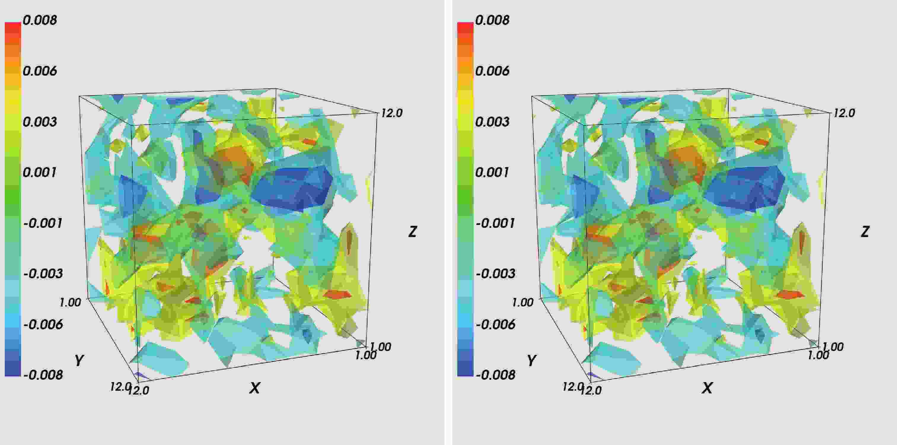
Before we proceed with the analysis, we first demonstrate that the SMP method with proper d is a good method to calculate the topological charge density with an overlap Dirac operator. When the source in the calculation of topological charge is a point source,
$ q_{{\rm ps}}\left(x\right) $ is an exact result of$ q_{{\rm ov}}\left(x\right) $ . It is reasonable to use$ q_{{\rm ps}}\left(x\right) $ as a benchmark for comparison. Due to the high computational cost, we only make a comparison of the point source and the SMP source in Eq. (6) on a$ 12^{3}\times24 $ lattice with$ \beta = 4.8 $ ,$ \kappa = 0.21 $ . We show$ q_{{\rm ps}}\left(x\right) $ obtained using the point source method and$ q_{{\rm smp}}\left(x\right) $ using the SMP method with$ d = 6 $ in Fig. 1. To show the visualization more clearly, we use a cutoff method, shown as the color map. The same cutoff procedure is used in other visualized figures. It shows that$ q_{{\rm smp}}\left(x\right) $ is highly matched with$ q_{{\rm ps}}\left(x\right) $ . The matching parameter$\Xi_{AB}$ for these two methods is$ 0.9997 $ , and we can barely see the difference with the naked eye. This shows that the error caused by the space-time off-diagonal elements of$ D_{\rm ov} $ is indeed very small when the distance parameter d of SMP source is proper. Thus, the SMP method is a good choice to calculate the topological charge density while the parameter d is large enough. It is expected that a better match corresponds to a larger distance d [16].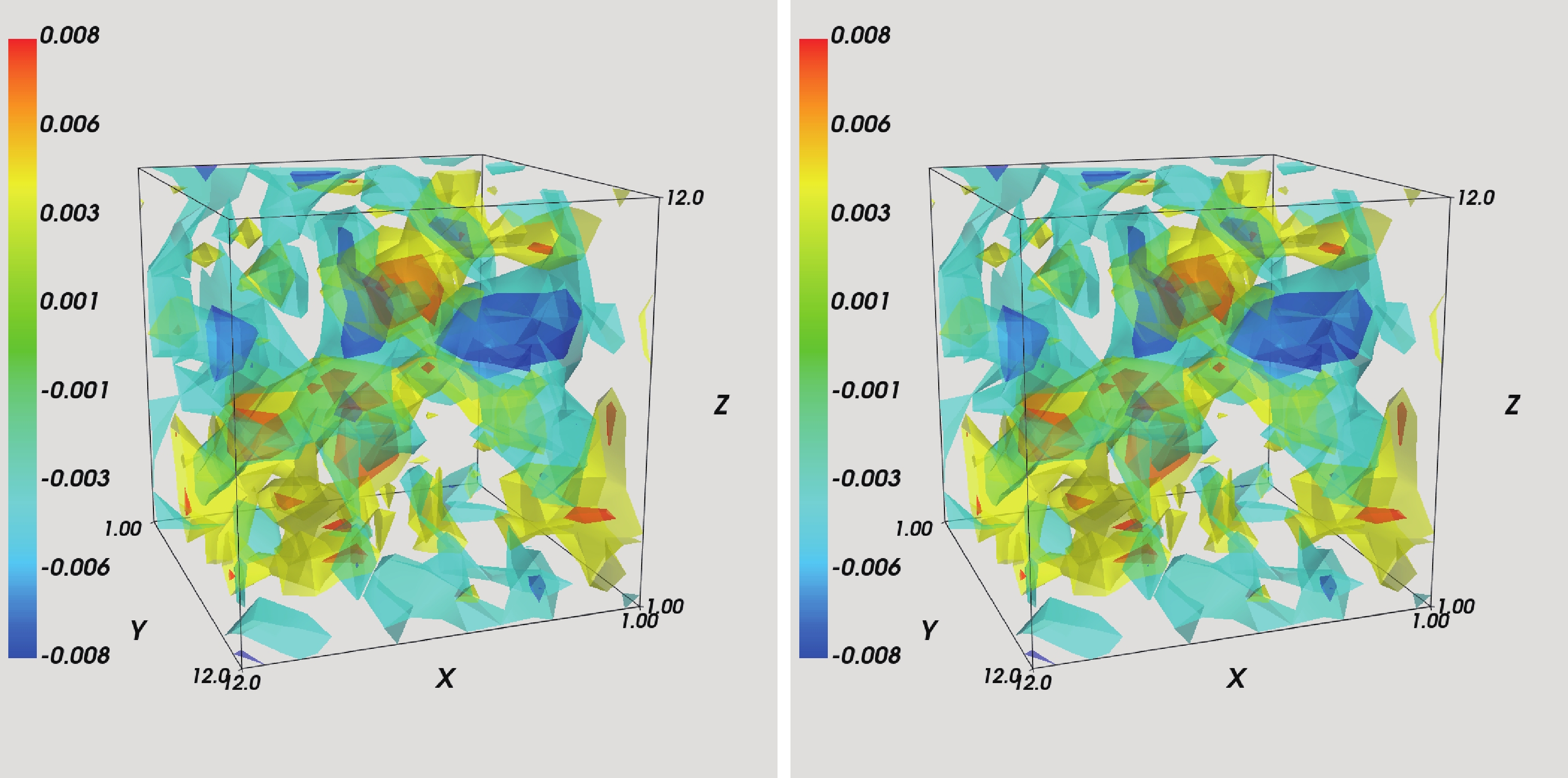
Figure 1. (color online)
$ q_{{\rm ps}}\left(x\right) $ and$ q_{{\rm smp}}\left(x\right) $ on lattice$ 12^{3}\times24 $ by the point source and SMP source for the$ t = 12 $ slice; other time slices are similar. To the naked eye, they are almost the same. The parameters$ \kappa = 0.21 $ and$ \beta = 4.80 $ are the same for both setups. In the figures, we use a color cutoff method shown as the color map. (left): Point source, (right): SMP source.To obtain more precise topological charge density, we choose the distance parameter
$ d = 8 $ in the SMP method on$ 16^{4} $ ,$ 24^{3}\times48 $ , and$ 32^{4} $ ensembles. The results are summarized in Tables 1-5. We only show the visualization of topological charge density$ q\left(x\right) $ for lattice volume$ 24^{3}\times48 $ at$ \beta = 4.80 $ as an example. The results for other lattice ensembles are similar. In these calculations of$ q\left(x\right) $ with$ d = 8 $ by the SMP method, we find that the topological charge$ Q_{\rm smp} $ is very close to an integer and it is not always the same for the same ensemble with different$ \kappa $ values. This is acceptable as zero crossings in the spectral flow of the$ \tilde{D}_{\text{ov}}\left(x\right) $ occur for different$ \kappa $ on the lattice [6, 18]. From the tables, it also shows that$ Q_{\rm smp} $ is very sensitive to$ \kappa $ on the coarsest lattice.$ Q_{\rm smp} $ changes a little on the finer lattice, and is stable versus the change of$ \kappa $ on the finest lattice. This sensitivity is probably the effect of finite lattice space a. All results indicate that even though the topological charge$ Q_{\rm smp} $ from overlap fermions is always an integer, its value is not unique, and it depends on the Wilson mass parameter m.$ \kappa $ 

$ \tau_{{\rm pr}} $ 

$ Z_{{\rm calc}} $ 

$\Xi_{ AB }$ 

$ Q_{{\rm smp}} $ 

$ Q_{\rm wf} $ 

$ 0.17 $ 

$ 0.360 $ 

$ 0.5121 $ 

$ 0.6853 $ 

$ 5.0010 $ 

3.5420 $ 0.18 $ 

$ 0.365 $ 

$ 0.7351 $ 

$ 0.7259 $ 

$ 5.0015 $ 

3.5299 $ 0.19 $ 

$ 0.350 $ 

$ 0.8656 $ 

$ 0.7309 $ 

$ 6.0005 $ 

3.5847 $ 0.21 $ 

$ 0.330 $ 

$ 1.0045 $ 

$ 0.7267 $ 

$ 3.9990 $ 

3.6378 $ 0.23 $ 

$ 0.320 $ 

$ 1.0073 $ 

$ 0.7030 $ 

$ 1.9963 $ 

3.6796 Table 1. Proper time of Wilson flow
$ \tau_{\rm pr} $ needed to match the SMP topological charge density with different$ \kappa $ at$ \beta = 4.50 $ and lattice volume$ 16^{4} $ for$ {\rm conf.}\thinspace1 $ .$ Q_{\rm smp} $ is obtained by the SMP method, and$ Q_{\rm wf} $ is the result of Wilson flow with$ \tau_{\rm pr}. $ $ \kappa $ 

$ \tau_{{\rm pr}} $ 

$ Z_{{\rm calc}} $ 

$\Xi_{ {AB} }$ 

$ Q_{{\rm smp}} $ 

$ Q_{\rm wf} $ 

$ 0.17 $ 

$ 0.365 $ 

$ 0.5230 $ 

$ 0.7006 $ 

$ -6.0091 $ 

−7.2945 $ 0.18 $ 

$ 0.360 $ 

$ 0.7235 $ 

$ 0.7339 $ 

$ -6.0052 $ 

−7.3027 $ 0.19 $ 

$ 0.350 $ 

$ 0.8680 $ 

$ 0.7471 $ 

$ -5.0026 $ 

−7.3181 $ 0.21 $ 

$ 0.330 $ 

$ 1.0077 $ 

$ 0.7322 $ 

$ -3.9997 $ 

−7.3458 $ 0.23 $ 

$ 0.320 $ 

$ 1.0121 $ 

$ 0.7096 $ 

$ -5.9964 $ 

−7.3581 Table 2. Proper time of Wilson flow
$ \tau_{\rm pr} $ needed to match the SMP topological charge density with different$ \kappa $ at$ \beta=4.50 $ and lattice volume$ 16^{4} $ for$ {\rm conf.}\thinspace2 $ .$ Q_{\rm smp} $ is obtained by the SMP method, and$ Q_{\rm wf} $ is the result of Wilson flow with$ \tau_{\rm pr}. $ $ \kappa $ 

$ \tau_{{\rm pr}} $ 

$ Z_{{\rm calc}} $ 

$\Xi_{ {AB} }$ 

$ Q_{{\rm smp}} $ 

$ Q_{\rm wf} $ 

$ 0.17 $ 

$ 0.365 $ 

$ 0.6811 $ 

$ 0.7653 $ 

$ 8.0077 $ 

8.5997 $ 0.18 $ 

$ 0.345 $ 

$ 0.8364 $ 

$ 0.7670 $ 

$ 7.0078 $ 

8.6863 $ 0.19 $ 

$ 0.325 $ 

$ 0.9275 $ 

$ 0.7580 $ 

$ 7.0095 $ 

8.7954 $ 0.21 $ 

$ 0.305 $ 

$ 1.0215 $ 

$ 0.7324 $ 

$ 9.0169 $ 

8.9322 $ 0.23 $ 

$ 0.295 $ 

$ 0.9811 $ 

$ 0.6972 $ 

$ 9.0279 $ 

9.0130 Table 3. Proper time of Wilson flow
$ \tau_{\rm pr} $ needed to match the SMP topological charge density with different$ \kappa $ at$ \beta=4.80 $ and lattice volume$ 24^{3}\times48 $ for$ {\rm conf.}\thinspace1 $ .$ Q_{\rm smp} $ is obtained by the SMP method, and$ Q_{\rm wf} $ is the result of Wilson flow with$ \tau_{\rm pr}. $ $ \kappa $ 

$ \tau_{{\rm pr}} $ 

$ Z_{{\rm calc}} $ 

$\Xi_{ {AB} }$ 

$ Q_{{\rm smp}} $ 

$ Q_{\rm wf} $ 

$ 0.17 $ 

$ 0.365 $ 

$ 0.6802 $ 

$ 0.7661 $ 

$ 4.9938 $ 

4.3224 $ 0.18 $ 

$ 0.345 $ 

$ 0.8359 $ 

$ 0.7656 $ 

$ 4.9932 $ 

4.3289 $ 0.19 $ 

$ 0.325 $ 

$ 0.9274 $ 

$ 0.7574 $ 

$ 3.9942 $ 

4.3365 $ 0.21 $ 

$ 0.305 $ 

$ 1.0211 $ 

$ 0.7309 $ 

$ 3.9949 $ 

4.3431 $ 0.23 $ 

$ 0.290 $ 

$ 0.9596 $ 

$ 0.6953 $ 

$ 3.9967 $ 

4.3454 Table 4. Proper time of Wilson flow
$ \tau_{\rm pr} $ needed to match the SMP topological charge density with varied$ \kappa $ at$ \beta=4.80 $ and lattice volume$ 24^{3}\times48 $ for$ {\rm conf.}\thinspace2 $ .$ Q_{\rm smp} $ is obtained by the SMP method, and$ Q_{\rm wf} $ is the result of Wilson flow with$ \tau_{\rm pr}. $ $ \kappa $ 

$ \tau_{{\rm pr}} $ 

$ Z_{{\rm calc}} $ 

$\Xi_{ {AB} }$ 

$ Q_{{\rm smp}} $ 

$ Q_{\rm wf} $ 

$ 0.17 $ 

$ 0.355 $ 

$ 0.7271 $ 

$ 0.7678 $ 

$ 3.0099 $ 

2.8066 $ 0.18 $ 

$ 0.335 $ 

$ 0.8724 $ 

$ 0.7627 $ 

$ 3.0059 $ 

2.7340 $ 0.19 $ 

$ 0.315 $ 

$ 0.9507 $ 

$ 0.7515 $ 

$ 3.0069 $ 

2.6380 $ 0.21 $ 

$ 0.295 $ 

$ 1.0233 $ 

$ 0.7222 $ 

$ 3.0127 $ 

2.5120 $ 0.23 $ 

$ 0.285 $ 

$ 0.9636 $ 

$ 0.6818 $ 

$ 3.0240 $ 

2.4352 Table 5. Proper time of Wilson flow
$ \tau_{\rm pr} $ needed to match the SMP topological charge density with varied$ \kappa $ at$ \beta=5.0 $ and lattice volume$ 32^{4} $ .$ Q_{\rm smp} $ is obtained by the SMP method, and$ Q_{\rm wf} $ is the result of Wilson flow with$ \tau_{\rm pr}. $ The SMP topological charge density for three choices
$ \kappa $ compared with the proper flow time of Wilson flow$ \tau_{{\rm pr}} $ for time slice$ t = 24 $ as an example is shown in Fig. 2, and$ q_{\text{wf}}\left(x\right) $ is renormalized using$ Z_{\rm {calc}} $ . Other time slices have a similar property. This shows that more Wilson flow time for$ q_{\text{wf}}\left(x\right) $ is needed to match the topological charge density$ q_{\text{smp}}\left(x\right) $ with a smaller$ \kappa $ or larger mass m. This phenomenon may be a result of the smaller$ \kappa $ showing sparser small eigenvalues of$ D_{\rm ov} $ , which has a similar effect of smoothing the configurations. However, the detailed reasons need further study. This indicates that the overlap Dirac operator is less sensitive to small objects as$ \kappa $ is decreased, and these objects can be removed by Wilson flow smoothing.
Figure 2. (color online) Best matched topological charge density
$ q_{\text{wf}}\left(x\right) $ (right) calculated by the Wilson flow method compared with the overlap$ q_{\text{smp}}\left(x\right) $ for the time slice$ t = 24 $ , where$ q_{\text{wf}}\left(x\right) $ is renormalized using$ Z_{\rm {calc}} $ .$ \tau_{\rm pr} $ is the proper flow time of Wilson flow fixed by a matching procedure. A color cutoff method is used shown as the color map in the figures.$ \tau_{\rm pr} $ ,$ Z_{\text{calc}} $ ,$ \Xi_{AB} $ ,$ Q_{\rm smp} $ and$ Q_{\rm wf} $ of different ensembles for five different$ \kappa $ are shown in Tables 1-5, respectively. When calculating$ Z_{{\rm calc}} $ , the flow time of Wilson flow is$ \tau_{\rm pr} $ . As the parameter$ \kappa $ increases, there is a monotonically decreasing trend in the proper flow time of Wilson flow in all tables. This shows that the matching procedure is effective and the proper flow time of Wilson flow is almost equal at the same$ \kappa $ for different configurations of the same lattice ensembles. When the parameter$ \kappa $ is fixed,$\Xi_{AB}$ and$ Z_{\text{calc}} $ are independent of topological charge Q and very close for different configurations with the same lattice volume. The value of$\Xi_{AB}$ is approximately in the range$ \left[0.68,0.77\right] $ . We can see that the proper flow time of Wilson flow$ \tau_{\rm pr} $ is different for different$ \kappa $ . However, it is reasonable to choose the average value of the proper flow time of Wilson flow of different$ \kappa $ as the proper$ \bar{\tau}_{\rm pr} $ . This is approximately$ \bar{\tau}_{\rm pr} = 0.345 $ ,$ \bar{\tau}_{\rm pr} = 0.327 $ ,$ \bar{\tau}_{\rm pr} = 0.317 $ , or the proper flow radius of Wilson flow$ \sqrt{8\tau} \approx 0.214 $ ,$ 0.137 $ and$ 0.104\thinspace{\text{fm}} $ for the lattice ensemble$ 16^{4} $ at$ \beta = 4.5 $ ,$ 24^{3}\times48 $ at$ \beta = 4.8 $ , and$ 32^{4} $ at$ \beta = 5.0 $ , respectively. This indicates that we can choose$ \bar{\tau}_{{\rm pr}} $ for gluonic$ q_{{\rm wf}}\left(x\right) $ to match with fermionic$ q_{{\rm smp}}\left(x\right) $ .All results show that
$ Q_{\rm wf} $ deviates largely from an integer for the proper flow time of Wilson flow fixed by the matching procedure. This phenomenon may be due to the fact that the topological charge is the global property of topological structure. However, the matching parameter$ \Xi_{AB} $ only shows the local matching property of topological charge density. Otherwise, the topological charge is the effect of the infrared properties, and the ultraviolet fluctuations lead to unphysical results as well as to non-integer topological charge values. Wilson flow is indeed a smoothing scheme of gauge fields. However, Wilson flow will modify the gauge field at the same time, which does not satisfy that the topological charge is conserved. In contrast,$ F_{\mu\nu}^{\text{Imp}} $ in Eq. (14) is applicable under the classical expansion with respect to lattice spacing a, and it may be affected by some quantum fluctuations even though the smoothing is performed.However, the topological charge is not the main quantity of interest, and the physically relevant observable is the topological susceptibility. The results show that to make the topological charge close to an integer, larger Wilson flow time is required. It is noted that too large a Wilson flow time may wipe out the negative core of the topological charge density correlator [31]. However, the flow time for the topological susceptibility to reach a plateau is smaller than the flow time for the topological charges reach some integers [28]. Nonetheless, the topological susceptibility using the SMP method is too expensive to calculated. In future work, we may try to consider it.
In Fig. 3,
$\Xi_{AB}$ versus the flow time of Wilson flow of one configuration for lattices of$ 16^4 $ ,$ 24^{3}\times48 $ , and$ 32^4 $ are shown.$\Xi_{AB}$ for other configurations have a similar trend. We see that as the flow time of Wilson flow$ \tau $ increases,$\Xi_{AB}$ reaches a maximum value and then decreases. When the parameter$ \kappa $ is fixed, we can observe that as the lattice spacing decreases, the proper flow time of Wilson flow almost uniformly decreases, as expected. It also shows that as the lattice spacing a decreases,$\Xi_{AB}$ tends to increase.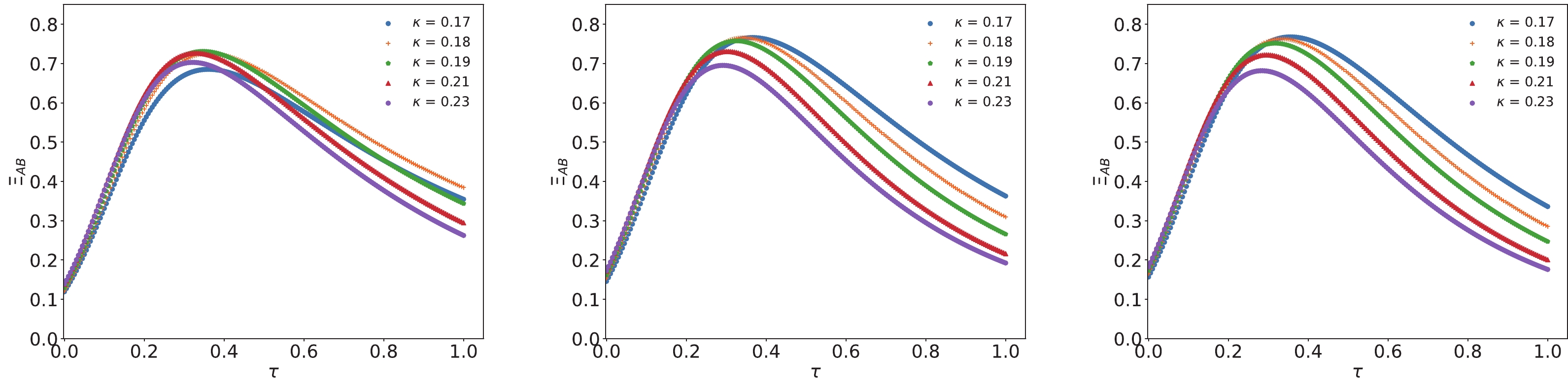
Figure 3. (color online)
$\Xi_{AB}$ versus$ \tau $ of one configuration for lattices of$ 16^4 $ ,$ 24^{3}\times48 $ and$ 32^4 $ . From left to right, the first figure is$\Xi_{AB}$ versus$ \tau $ for lattice volume$ 16^{4} $ , the second figure for lattice volume$ 24^{3}\times48 $ , and the last one for lattice volume$ 32^{4} $ . As$ \kappa $ is reduced, the proper flow time of Wilson flow is increased. As the lattice spacing decreases,$\Xi_{AB}$ tends to increase. -
We have analyzed the topological charge density
$ q\left(x\right) $ of all time slices using direct visualizations. We find that the SMP method is a good choice to study the topological charge density in the fermionic definition, and the SMP method is much cheaper than the traditional point source method, especially for a large lattice volume. The results show that the topological charge density depends on the Wilson mass parameter m in the fermionic definition. By comparing the$ q_{{\rm smp}}\left(x\right) $ with the gluonic definition of$ q_{{\rm wf}}\left(x\right) $ , a correlation between m and$ \tau $ is revealed. Smaller values of$ \kappa $ remove non-trivial topological charge fluctuations, which are similar to Wilson flow with a larger flow time. The detailed reasons are worthy of further study. By analyzing the topological charge density$ q\left(x\right) $ , we find that the proper flow time of Wilson flow for the gluonic definition of topological charge density can be obtained by the comparison of$ q_{{\rm smp}}\left(x\right) $ with$ q_{{\rm wf}}\left(x\right) $ . We also observe that the proper flow time of Wilson flow decreases with the decrease in lattice spacing a, which is consistent with expectations. Furthermore, as the lattice spacing a decreases,$\Xi_{AB}$ tends to increase.We also find that the topological charge obtained by Wilson flow at the proper flow time is far from an integer, and it is different from that of the fermionic definition. Although the topological charge density of the fermionic definition and that of the gluonic definition have the best match, the topological charge from the fermionic and gluonic definition are very different. The reason for this phenomenon may be that the matching parameter
$ \Xi_{AB} $ only shows the local matching property of topological charge density, but the topological charge is the global property of topological structure. In contrast, Wilson flow can indeed smooth the gauge field. However, Wilson flow also changes the configurations, which does not guarantee the conservation of topological charge. Otherwise, in the gluonic definition of topological charge density, we used the improved field strength tensor corrected in the classical expansion with respect to lattice spacing, which may be affected by the quantum fluctuations even though the Wilson flow is used. The detailed reasons need further study.In the SMP method, we had known that the error is dependent on the off-diagonal components of the overlap operator. With a larger distance parameter, it has smaller errors in the SMP method. We can try to choose a larger distance parameter to decrease the error in future work. Otherwise, we could try to improve the field strength tensor to reduce the effect of classical expansion with respect to the lattice spacing in the gluonic definition of topological charge density.
-
We are grateful to Heng-tong Ding for careful reading of the manuscript and useful suggestions. Numerical simulations have been performed on the Tianhe-2 supercomputer at the National Supercomputer Center in Guangzhou (NSCC-GZ), China.
Dependence of overlap topological charge density on Wilson mass parameter
- Received Date: 2021-03-07
- Available Online: 2021-07-15
Abstract: In this paper, we analyze the dependence of the topological charge density from the overlap operator on the Wilson mass parameter in the overlap kernel by the symmetric multi-probing source (SMP) method. We observe that non-trivial topological objects are removed as the Wilson mass is increased. A comparison of topological charge density calculated by the SMP method using the fermionic definition with that of the gluonic definition by the Wilson flow method is shown. A matching procedure for these two methods is used. We find that there is a best match for topological charge density between the gluonic definition with varied Wilson flow time and the fermionic definition with varied Wilson mass. By using the matching procedure, the proper flow time of Wilson flow in the calculation of topological charge density can be estimated. As the lattice spacing a decreases, the proper flow time also decreases, as expected.


 DownLoad: