


 Abstract
 HTML
HTML Reference
 Related
 PDF
PDF


-
The objective of the study of hadrons is to reveal the possible degrees of freedom responsible for the appearance of a given system. The quark confinement and asymptotic freedom have been the starting points of any theoretical and phenomenological study to understand quark dynamics. Hadron spectroscopy attempts to explore the excited mass spectrum along with the multiplet structure and spin-parity assignments. The light quark baryons form the basis of octets and decuplets ranging from strangeness S = 0 to S = −3 based on symmetric, asymmetric, and mixed-symmetric flavor-spin combinations.
$ 3 \otimes 3 \otimes 3 = 1^{A} \oplus 8^{M} \oplus 8^{M} \oplus 10^{S}. $

The presence of a strange quark in a baryon draws attention because it would be slightly heavier than u and d quarks and considerably lighter than c and b quarks. Particularly, the strangeness S = −2
$ \Xi $ baryons have not been observed experimentally like other light sector baryons [1], as depicted in Table 1. The limited observations in the$ \Xi $ baryon group are owing to the fact that they are produced only as the final state in a process in addition to having considerably small cross-sections [2]. Unlike the$ \Xi $ baryons,$ \Sigma $ and$ \Lambda $ with S = −1 have quite a number of experimentally established states.State $J^{P}$ 

Status $\Xi^{0}$ (1314)

$\dfrac{1}{2}^{+}$ 

**** $\Xi^{-}$ (1321)

$\dfrac{1}{2}^{+}$ 

**** $\Xi$ (1530)

$\dfrac{3}{2}^{+}$ 

**** $\Xi$ (1620)

* $\Xi$ (1690)

*** $\Xi$ (1820)

$\dfrac{3}{2}^{-}$ 

*** $\Xi$ (1950)

*** $\Xi$ (2030)

$\dfrac{5}{2}^{?}$ 

*** $\Xi$ (2120)

* $\Xi$ (2250)

** $\Xi$ (2370)

** $\Xi$ (2500)

* Table 1.
$\Xi$ listed by Particle Data Group (PDG [1]).The present article is dedicated to the study of
$ \Lambda $ ,$ \Sigma $ and$ \Xi $ baryons. Cascade baryons appear with isospin$ I = \dfrac{1}{2} $ in the octet ($ J = \dfrac{1}{2} $ ) and decuplet ($ J = \dfrac{3}{2} $ ) as$ \Xi $ and$ \Xi^{*} $ , respectively. The quark combination is uss for$ \Xi^{0} $ and dss for$ \Xi^{-} $ .For mixed symmetry flavor wave-function in the octet group,
$ \begin{aligned}[b] &{\Xi^{0} \rightarrow \quad \dfrac{1}{\sqrt{6}}(sus+uss-2ssu)},\\ &{\Xi^- \rightarrow \quad \dfrac{1}{\sqrt{6}}(dss+sds-2ssd)},\\ &{ \Xi^{0} \rightarrow \quad \dfrac{1}{\sqrt{2}}(uss-sus)},\\ &{\Xi^- \rightarrow \quad \dfrac{1}{\sqrt{2}}(dss-sds). } \end{aligned} $

For symmetric flavor wave-function in the decuplet group,
$ \begin{aligned}[b] &{ \Xi^{*0} \rightarrow \quad \dfrac{1}{\sqrt{3}}(uss+sus+ssu) },\\ &{ \Xi^{*-} \rightarrow \quad \dfrac{1}{\sqrt{3}}(dss+sds+ssd)}. \end{aligned} $

Similarly, the
$ \Sigma $ baryon with u, d, and s constituent quarks has a place in octets and decuplets with three possible combinations as uus, uds, and dds respectively. The$ \Lambda $ baryon appearing in an octet as I = 0 has uds quark content; however, its wave-function differs from that of$ \Sigma^{0} $ .Experimental facilities around the world have been striving to study strange hyperons. A recent study at CERN by ALICE Collaboration established an attractive interaction between protons and
$ \Xi^{-} $ [3]. Activities in measuring weak decays of$ \Xi $ hyperons were reported by the KTeV Collaboration [4] and the NA48/1 Collaboration [5]; the BABAR Collaboration has also been carrying out extensive studies [6]. The photoproduction of$ \Xi $ has been observed by CLAS detector at Jefferson Lab [7]. Additionally, JLab has recently proposed to explore the strange hyperon spectroscopy through a secondary KL beam along with a GlueX experiment [8], and the findings are expected to provide new direction and understanding of strange hyperons$ \Sigma $ ,$ \Lambda $ , and$ \Xi $ . The BESIII Collaboration observed$ \Xi $ (1530) in a baryon-antibaryon pair from charmonium decay [9]. The upcoming experimental facility PANDA at FAIR-GSI has high expectations to establish the whole spectrum of hyperons through proton-antiproton collisions [10-13]. A$ \Xi $ dedicated study has been undertaken for mass, width, and decay modes by a member of the PANDA group [14-16].In the case of
$ \Sigma $ and$ \Lambda $ baryons, all properties are not completely known. Most of the data for strange baryons have been based on earlier studies from a bubble chamber for$ K^{-} $ reactions. The$ \Lambda $ (1405) with$ J^{P} = \dfrac{1}{2}^{-} $ is still a mysterious state in the lambda spectrum. This state is lower than the non-strange counterpart$ N^{*} $ (1535). Recent studies have attempted to understand this state as hadronic molecular [17, 18]. The JPAC and Osaka-ANL groups have applied a coupled channel approach to study these dynamics [19, 20]. Additionally, a two pole structure of$ \Lambda $ (1405) has been analyzed using chiral effective field theory [21]. E. Klempt et al. has extensively reviewed the$ \Lambda $ and$ \Sigma $ hyperon spectrum based on experimental and theoretical studies focusing on all the known states of the spectrum [22]. These spectra are studied through photoproduction off the proton in ref. [23]. The study of strangeness S = −1 and −2 becomes more interesting not only in a high energy arena but also in astrophysical bodies such as neutron stars [24].The excited states of hyperons have been investigated using phenomenological as well as theoretical approaches. Various models have attempted to reproduce the octet and decuplet ground states and a range of excited states. A recent review has summarized in detail a few strange baryon spectrum states with theoretical and experimental aspects [25]. L. Xiao et al. intensively studied the strong decays of
$ \Xi $ under the chiral quark model, which may assist in determining the possible spin-parity of a given state in strong decay [26]. Some of the models have been summarized briefly in Sec. 3, ranging from the relativistic approach [27], instanton induced model [28], CI model [29], algebraic model [30], and Skyrme model [31], etc. The present work is based on the phenomenological non-relativistic hypercentral constituent quark model [32]. Similar studies have previously been carried out for nucleons and delta baryons, which serve as guides towards exploring strange baryons [33-36].This paper is organized as follows: after the briefing on hadron spectroscopy and various experimental and theoretical approaches, Sec. 2 deals with the background of the model used. Sec. 3 describes the results for resonance masses and provides a detailed discussion regarding the data presented in respective tables. Sec. 4 presents the Regge trajectories and deductions based on them. Sec. 5 is dedicated to the magnetic moments of the isospin states of
$ \Xi $ ,$ \Sigma $ , and$ \Lambda $ based on their effective masses. Sec. 6 focuses on the transition magnetic moments and radiative decay widths, and lastly, the conclusion ends the paper. -
The constituent quark model (CQM) is based on a simple assumption of baryon as a system of three quarks (or anti-quarks) interacting by some potential, which ultimately may provide a quantitative description of baryonic properties. It is obvious that the QCD quark masses are considerably smaller than constituent quark masses; however, this large mass parametrizes all the other effects in a baryon. Thus, the CQMs have been employed in various studies through various modifications in non-relativistic or semi-relativistic approaches.
The hypercentral constituent quark model (hCQM) has been employed for the present study, which is a non relativistic approach [37, 38]. It undertakes the baryon as a confined system of three quarks wherein the potential is hypercentral one. The dynamics of a three body system are addressed using the Jacobi coordinates, introduced as
$ \rho $ and$ \lambda $ , reducing the body parameters to two [39].$ {{\bf{\rho}}} = \dfrac{1}{\sqrt{2}}({{{r}}_{\bf{1}}} -{{{r}}_{\bf{2}}}), $

(1) $ {{\bf{\lambda}}} = \dfrac{(m_{1}{{{r}}_{\bf{1}}} + m_{2}{{{r}}_{\bf{2}}} - (m_{1}+m_{2}){{{r}}_{\bf{3}}})}{\sqrt{m_{1}^{2} + m_{2}^{2} + (m_{1}+m_{2})^{2}}}. $

(2) The hyperradius and hyperangle are defined as
$ x = \sqrt{{{\bf{\rho}}^{2}} + {{\bf{\lambda}}^{2}}} ; \; \;\;\;\; \xi = {\rm arctan}\left(\dfrac{\rho}{\lambda}\right). $

(3) The Hamiltonian of the system is written with the potential term solely depending on the hyperradius x of the three body system
$ H = \dfrac{P^{2}}{2m} + V^{0}(x) + V_{\rm SD}(x), $

(4) where
$ m = \dfrac{2m_{\rho}m_{\lambda}}{m_{\rho}+m_{\lambda}} $ is the reduced mass. Thus the hyper-radial part of the wave-function as determined by the hypercentral Schrodinger equation is [40]$ \left[\dfrac{{\rm d}^{2}}{{\rm d}x^{2}} + \dfrac{5}{x}\dfrac{\rm d}{{\rm d}x} - \dfrac{\gamma(\gamma +4)}{x^{2}}\right]\psi(x) = -2m[E-V(x)]\psi(x). $

(5) Here,
$ \gamma $ replaces the angular momentum quantum number with the relation$ l(l+1) \rightarrow \dfrac{15}{4} + \gamma (\gamma + 4) $ . The choice of hypercentral potential narrows down to a hyperCoulomb one, i.e.,$ -\dfrac{\tau}{x} $ . The confinement term here is chosen to be of linear nature.$ V^{0}(x) = -\dfrac{\tau}{x} + \alpha x. $

(6) Here,
$ \tau = \dfrac{2}{3}\alpha_{s} $ , with$ \alpha_{s} $ being a running coupling constant and$ \alpha $ a parameter based on the fitting of the ground state for a given system.The
$ V_{\rm SD}(x) $ accounts for the spin-dependent terms leading to hyperfine interactions.$ \begin{aligned}[b] V_{SD}(x) =& V_{SS}(x)({{{S}}_{\bf{\rho}}}\cdot {{S}}_{\bf{\lambda}}) + V_{\gamma S}(x)({{\bf{\gamma}} \cdot {{S}}}) \\ &+ V_{T}\times \left[S^{2}- \dfrac{3({{{S}}\cdot {{x}}})({{{S}}\cdot {{x}}})}{x^{2}}\right]. \end{aligned} $

(7) where
$ V_{SS}(x) $ ,$ V_{\gamma S}(x) $ , and$ V_{T}(x) $ are spin-spin, spin-orbit, and tensor terms, respectively [41]. In the present study, a first order correction term to the potential with$ \dfrac{1}{m} $ dependence has also been added as$ \dfrac{1}{m}V^{1}(x) $ [42-44].$ V^{1}(x) = -C_{F}C_{A}\dfrac{\alpha_{s}^{2}}{4x^{2}}, $

(8) where
$ C_{F} $ and$ C_{A} $ are Casimir elements of fundamental and adjoint representation.The resonance masses have been obtained with and without the first order correction term. The constituent quark masses have been taken to be
$ m_{u} = m_{d} = 0.290 $ MeV and$ m_{s} = 0.500 $ MeV. Mathematica Notebook has been employed for numerical solutions [45]. -
In the present work, the resonance masses are calculated for radial and orbital states from 1S-5S, 1P-4P, 1D-3D, and 1F-2F. In Tables 2-20, the resonance mass for all the possible spin-parity configurations for each state with
$ S = \dfrac{1}{2} $ and$ S = \dfrac{3}{2} $ has been considered and the respective contribution has been calculated based on the model discussed in Sec. 2, including with and without first order corrections. For S-state, possible total angular momentum and parity are$ \dfrac{1}{2}^{+} $ and$ \dfrac{3}{2}^{+} $ (Tables 2, 8, and 15); for P-state, the range goes from$ \dfrac{1}{2}^{-} $ to$ \dfrac{5}{2}^{-} $ (Tables 3, 9, and 16); for D-state, the range is$ \dfrac{3}{2}^{+} $ to$ \dfrac{7}{2}^{+} $ (Tables 4, 10, and 17); and for F-state, it is$ \dfrac{3}{2}^{-} $ to$ \dfrac{9}{2}^{-} $ (Tables 5, 11, and 18). Additionally, for G-state, the range is from$ \dfrac{5}{2}^{+} $ to$ \dfrac{11}{2}^{+} $ (Table 12) (only calculated for baryon). Only a few experimentally established states with four star status availability are mentioned in their respective tables. In the tables,$ Mass_{\rm cal}1 $ and$ Mass_{\rm cal}2 $ represent resonance masses without and with first order correction, respectively, in MeV.State $J^{P}$ 

$Mass_{\rm cal}$ 1

$Mass_{\rm cal}$ 2

$Mass_{\rm exp}$ [1]

1S $\dfrac{1}{2}^{+}$ 

1322 1321 1321 $\dfrac{3}{2}^{+}$ 

1531 1524 1532 2S $\dfrac{1}{2}^{+}$ 

1884 1891 $\dfrac{3}{2}^{+}$ 

1971 1964 3S $\dfrac{1}{2}^{+}$ 

2361 2372 $\dfrac{3}{2}^{+}$ 

2457 2459 4S $\dfrac{1}{2}^{+}$ 

2935 2954 $\dfrac{3}{2}^{+}$ 

3029 3041 5S $\dfrac{1}{2}^{+}$ 

3591 3620 $\dfrac{3}{2}^{+}$ 

3679 3702 Table 2. S-wave of
$\Xi$ baryon (in MeV).State $J^{P}$ 

$Mass_{\rm cal}$ 1

$Mass_{\rm cal}$ 2

$Mass_{\rm exp}$ [1]

$1^{2}P_{1/2}$ 

$\dfrac{1}{2}^{-}$ 

1886 1889 $1^{2}P_{3/2}$ 

$\dfrac{3}{2}^{-}$ 

1871 1873 1823 $1^{4}P_{1/2}$ 

$\dfrac{1}{2}^{-}$ 

1894 1897 $1^{4}P_{3/2}$ 

$\dfrac{3}{2}^{-}$ 

1879 1881 1823 $1^{4}P_{5/2}$ 

$\dfrac{5}{2}^{-}$ 

1859 1859 $2^{2}P_{1/2}$ 

$\dfrac{1}{2}^{-}$ 

2361 2373 $2^{2}P_{3/2}$ 

$\dfrac{3}{2}^{-}$ 

2337 2347 $2^{4}P_{1/2}$ 

$\dfrac{1}{2}^{-}$ 

2373 2386 $2^{4}P_{3/2}$ 

$\dfrac{3}{2}^{-}$ 

2349 2360 $2^{4}P_{5/2}$ 

$\dfrac{5}{2}^{-}$ 

2318 2325 $3^{2}P_{1/2}$ 

$\dfrac{1}{2}^{-}$ 

2929 2948 $3^{2}P_{3/2}$ 

$\dfrac{3}{2}^{-}$ 

2894 2913 $3^{4}P_{1/2}$ 

$\dfrac{1}{2}^{-}$ 

2946 2966 $3^{4}P_{3/2}$ 

$\dfrac{3}{2}^{-}$ 

2912 2931 $3^{4}P_{5/2}$ 

$\dfrac{5}{2}^{-}$ 

2865 2884 $4^{2}P_{1/2}$ 

$\dfrac{1}{2}^{-}$ 

3577 3609 $4^{2}P_{3/2}$ 

$\dfrac{3}{2}^{-}$ 

3532 3563 $4^{4}P_{1/2}$ 

$\dfrac{1}{2}^{-}$ 

3599 3632 $4^{4}P_{3/2}$ 

$\dfrac{3}{2}^{-}$ 

3554 3586 $4^{4}P_{5/2}$ 

$\dfrac{5}{2}^{-}$ 

3494 3524 Table 3. P-wave of
$\Xi$ baryon (in MeV).State $J^{P}$ 

$Mass_{\rm cal}$ 1

$Mass_{\rm cal}$ 2

$Mass_{\rm exp}$ [1]

$1^{2}D_{3/2}$ 

$\dfrac{3}{2}^{+}$ 

2270 2281 $1^{2}D_{5/2}$ 

$\dfrac{5}{2}^{+}$ 

2234 2244 $1^{4}D_{1/2}$ 

$\dfrac{1}{2}^{+}$ 

2310 2322 $1^{4}D_{3/2}$ 

$\dfrac{3}{2}^{+}$ 

2283 2295 $1^{4}D_{5/2}$ 

$\dfrac{5}{2}^{+}$ 

2247 2257 $1^{4}D_{7/2}$ 

$\dfrac{7}{2}^{+}$ 

2203 2211 $2^{2}D_{3/2}$ 

$\dfrac{3}{2}^{+}$ 

2819 2842 $2^{2}D_{5/2}$ 

$\dfrac{5}{2}^{+}$ 

2771 2791 $2^{4}D_{1/2}$ 

$\dfrac{1}{2}^{+}$ 

2874 2899 $2^{4}D_{3/2}$ 

$\dfrac{3}{2}^{+}$ 

2838 2861 $2^{4}D_{5/2}$ 

$\dfrac{5}{2}^{+}$ 

2790 2810 $2^{4}D_{7/2}$ 

$\dfrac{7}{2}^{+}$ 

2729 2747 $3^{2}D_{3/2}$ 

$\dfrac{3}{2}^{+}$ 

3455 3489 $3^{2}D_{5/2}$ 

$\dfrac{5}{2}^{+}$ 

3391 3423 $3^{4}D_{1/2}$ 

$\dfrac{1}{2}^{+}$ 

3527 3562 $3^{4}D_{3/2}$ 

$\dfrac{3}{2}^{+}$ 

3479 3513 $3^{4}D_{5/2}$ 

$\dfrac{5}{2}^{+}$ 

3415 3448 $3^{4}D_{7/2}$ 

$\dfrac{7}{2}^{+}$ 

3336 3366 Table 4. D-wave of
$\Xi$ baryon (in MeV).$J^{P}$ 

$Mass_{\rm cal}1$ 

$Mass_{\rm cal}2$ 

[27] [28] [29] [30] [46] [47] [31] [2] [48] [49] $\dfrac{1}{2}^{+}$ 

1322 1321 1330 1310 1305 1334 1348 1317 1318 1325 1317 1303 ± 13 1884 1891 1886 1876 1840 1727 1805 1772 1932 1891 1750 2178 ± 48 2310 2322 1993 2062 2040 1932 1868 1980 2231 ± 44 2361 2372 2012 2131 2100 1874 2054 2408 ± 45 2874 2899 2091 2176 2130 2107 2935 2954 2142 2215 2150 2149 3527 3562 2367 2249 2230 2254 3591 3620 2345 $\dfrac{3}{2}^{+}$ 

1531 1524 1518 1539 1505 1524 1528 1552 1539 1520 1526 1553 ± 18 1971 1964 1966 1988 2045 1878 1653 2120 1934 1952 2228 ± 40 2270 2281 2100 2076 2065 1979 1970 2398 ± 52 2283 2295 2121 2128 2115 2065 2574 ± 52 2457 2459 2122 2170 2165 2114 2819 2842 2144 2175 2170 2174 2838 2861 2149 2219 2210 2184 3029 3041 2421 2257 2230 2218 3455 3489 2279 2275 2252 3479 3513 3679 3702 $\dfrac{5}{2}^{+}$ 

2234 2242 2108 2013 2045 1936 1959 2247 2295 2147 2141 2165 2025 2102 2771 2791 2213 2197 2230 2170 2790 2810 2231 2230 2205 3391 3423 2279 2240 2239 3415 3448 $\dfrac{7}{2}^{+}$ 

2203 2211 2189 2169 2180 2035 2074 2729 2747 2289 2240 2189 3336 3366 Table 6. Comparison of masses with other predictions based on
$J^{P}$ value for$\Xi$ baryon (in MeV).$J^{P}$ 

$Mass_{\rm cal}1$ 

$Mass_{\rm cal}2$ 

[27] [28] [29] [30] [46] [47] [31] [2] [48] [49] $\dfrac{1}{2}^{-}$ 

1886 1889 1682 1770 1755 1869 1658 1725 1772 1716 ± 43 1894 1897 1758 1922 1810 1932 1811 1894 1837 ± 28 2361 2373 1839 1938 1835 2076 1926 1844 ± 43 2373 2386 2160 2241 2225 2758 ± 78 2929 2948 2210 2266 2285 2946 2966 2233 2387 2300 3577 3609 2261 2411 2320 3599 3632 2445 2380 Continued on next page Table 7. Comparison of masses with other predictions based on
$J^{P}$ value for$\Xi$ baryon (in MeV).State $J^{P}$ 

$Mass_{\rm cal}$ 1

$Mass_{\rm cal}$ 2

$Mass_{\rm exp}$ [1]

1S $\dfrac{1}{2}^{+}$ 

1115 1115 1115 2S $\dfrac{1}{2}^{+}$ 

1592 1589 1600 3S $\dfrac{1}{2}^{+}$ 

1885 1892 1810 4S $\dfrac{1}{2}^{+}$ 

2202 2220 5S $\dfrac{1}{2}^{+}$ 

2540 2571 Table 8. S-wave of
$\Lambda$ baryon (in MeV).$J^{P}$ 

$Mass_{\rm cal}1$ 

$Mass_{\rm cal}2$ 

[27] [28] [29] [30] [46] [47] [50] [51] [48] [49] $\dfrac{1}{2}^{+}$ 

1115 1115 1115 1108 1115 1133 1136 1116 1116 1112 1113 1149 ± 18 1592 1589 1615 1677 1680 1577 1625 1518 1600 1695 1606 1807 ± 94 1794 1814 1799 1799 1666 1810 1764 2112 ± 54 1885 1892 1901 1747 1830 1955 1880 2137 ± 68 2105 2144 1972 1898 1910 1960 2013 2202 2220 1986 2077 2010 2173 2441 2496 2042 2099 2105 2198 2540 2571 2099 2132 2120 $\dfrac{3}{2}^{+}$ 

1769 1789 1854 1823 1900 1849 1896 1890 1903 1836 1991 ± 103 1777 1798 1976 1952 1960 2000 1958 2058 ± 139 2076 2113 2130 2045 1995 1993 2481 ± 111 2086 2123 2184 2087 2050 2061 2408 2459 2202 2133 2080 2121 2419 2471 2134 $\dfrac{5}{2}^{+}$ 

1746 1767 1825 1834 1890 1849 1896 1820 1846 1839 1755 1776 2098 1999 2035 2074 2110 2132 2008 2051 2085 2221 2078 2115 2103 2060 2096 2255 2127 2115 2129 2305 2363 2258 2150 2180 2155 2378 2426 2389 2471 $\dfrac{7}{2}^{+}$ 

1727 1748 2251 2130 2120 2020 2064 2029 2061 2471 2331 2253 2302 2265 2316 2352 2398 $\dfrac{9}{2}^{+}$ 

2204 2246 2360 2340 2357 2350 2360 2216 2260 $\dfrac{11}{2}^{+}$ 

2159 2195 2585 Table 13. Comparison of masses with other predictions based on
$J^{P}$ value for$\Lambda$ baryon (in MeV).$J^{P}$ 

$Mass_{\rm cal}1$ 

$Mass_{\rm cal}2$ 

[27] [28] [29] [30] [46] [47] [50] [51] [48] [49] $\dfrac{1}{2}^{-}$ 

1546 1558 1406 1524 1550 1686 1556 1650 1670 1679 1559 1416 ± 81 1553 1564 1667 1630 1615 1799 1682 1732 1830 1656 1546 ± 110 1834 1858 1733 1816 1675 1778 1969 1800 1791 1713 ± 116 1841 1867 1927 2011 2015 1854 2075 ± 249 2149 2186 2197 2076 2095 1928 2158 2196 2218 2117 2160 2484 2536 2495 2548 $\dfrac{3}{2}^{-}$ 

1534 1544 1549 1508 1545 1686 1556 1650 1690 1683 1560 1751 ± 41 1540 1551 1693 1662 1645 1682 1785 1520 1702 2203 ± 106 1819 1841 1812 1775 1770 1854 2325 1859 2381 ± 87 1827 1850 2035 1987 2030 1928 2043 2079 2319 2090 2110 1969 2131 2166 2322 2147 2185 2140 2176 2392 2259 2230 2371 2427 2454 2290 2275 2464 2513 2468 2313 2474 2525 2723 2793 $\dfrac{5}{2}^{-}$ 

1524 1533 1807 1827 1861 1828 1775 1799 1778 1785 1830 1850 1803 2005 2039 2136 2080 2180 2015 2050 2350 2179 2250 2116 2149 2329 2380 2341 2393 2447 2494 2676 2741 2689 2755 $\dfrac{7}{2}^{-}$ 

1970 2002 2097 2090 2150 2100 2087 1980 2013 2583 2227 2230 2291 2337 2303 2350 2632 2693 2645 2707 $\dfrac{9}{2}^{-}$ 

1939 1969 2665 2370 2257 2299 2593 2650 Table 14. Comparison of masses with other predictions based on
$J^{P}$ value for$\Lambda$ baryon (in MeV).State $J^{P}$ 

$Mass_{\rm cal}$ 1

$Mass_{\rm cal}$ 2

$Mass_{\rm exp}$ [1]

1S $\dfrac{1}{2}^{+}$ 

1193 1193 1193 $\dfrac{3}{2}^{+}$ 

1384 1384 1385 2S $\dfrac{1}{2}^{+}$ 

1643 1643 1660 $\dfrac{3}{2}^{+}$ 

1827 1827 3S $\dfrac{1}{2}^{+}$ 

2083 2099 $\dfrac{3}{2}^{+}$ 

2229 2236 4S $\dfrac{1}{2}^{+}$ 

2560 2589 $\dfrac{3}{2}^{+}$ 

2675 2693 5S $\dfrac{1}{2}^{+}$ 

3067 3108 $\dfrac{3}{2}^{+}$ 

3159 3189 Table 15. S-wave of
$\Sigma$ baryon (in MeV).$J^{P}$ 

$Mass_{\rm cal}1$ 

$Mass_{\rm cal}2$ 

[27] [28] [29] [30] [46] [47] [50] [51] [48] [49] $\dfrac{1}{2}^{+}$ 

1193 1193 1187 1190 1190 1170 1180 1211 1193 1198 1192 1216 ± 15 1643 1643 1711 1760 1720 1604 1616 1546 1660 1656 1664 2069 ± 74 2083 2099 1922 1947 1915 1911 1668 1770 1924 2149 ± 66 2086 2107 1983 2009 1970 1801 1880 1986 2335 ± 63 2536 2568 2028 2052 2005 2022 2560 2589 2180 2098 2030 2069 3027 3072 2292 2138 2105 2172 3067 3108 2472 3549 3613 $\dfrac{3}{2}^{+}$ 

1384 1384 1381 1411 1370 1382 1389 1334 1385 1381 1383 1471 ± 23 1827 1827 1862 1896 1920 1865 1439 1560 1868 2194 ± 81 2040 2057 2025 1961 1970 1924 1690 1947 2250 ± 79 2055 2074 2076 2011 2010 1840 1993 2468 ± 67 2229 2236 2096 2044 2030 2039 2481 2510 2157 2062 2045 2075 2499 2529 2186 2103 2085 2098 2675 2693 2112 2115 2122 2962 3004 2168 2984 3027 3159 3189 $\dfrac{5}{2}^{+}$ 

1998 2013 1991 1956 1995 1872 2061 1915 1930 1949 2014 2029 2062 2027 2030 2070 2028 2432 2459 2221 2071 2095 2062 2451 2478 2107 2905 2945 2154 2926 2967 3410 3464 3435 3490 $\dfrac{7}{2}^{+}$ 

1962 1974 2033 2070 2060 2012 2030 2039 2002 2390 2414 2470 2161 2125 2106 2855 2892 3353 3403 Table 19. Comparison of masses with other predictions based on
$J^{P}$ value for$\Sigma$ baryon (in MeV).$J^{P}$ 

$Mass_{\rm cal}1$ 

$Mass_{\rm cal}2$ 

[27] [28] [29] [30] [46] [47] [50] [51] [48] [49] $\dfrac{1}{2}^{-}$ 

1720 1725 1620 1628 1630 1711 1677 1753 1620 1754 1657 1603 ± 38 1731 1736 1693 1771 1675 1736 1868 1750 1746 1718 ± 58 2128 2145 1747 1798 1695 1759 1895 2000 1802 1730 ± 34 2142 2159 2115 2111 2110 2478 ± 104 2580 2608 2198 2136 2155 2598 2627 2202 2251 2165 3068 3111 2289 2264 2205 3088 3133 2381 2288 2260 3588 3641 3612 3664 $\dfrac{3}{2}^{-}$ 

1698 1702 1706 1669 1655 1711 1677 1753 1670 1697 1698 1861 ± 26 1709 1713 1731 1728 1750 1974 1736 1868 1940 1956 1790 1736 ± 40 2099 2114 1856 1781 1755 1759 1895 2250 1802 2394 ± 74 2114 2129 2175 2139 2120 2297 ± 122 2416 2495 2203 2171 2185 2545 2571 2300 2203 2200 2563 2589 2943 2990 3027 3067 3047 3089 3456 3512 3541 3594 3565 3617 $\dfrac{5}{2}^{-}$ 

1680 1683 1757 1770 1755 1736 1753 1775 1777 1743 2076 2087 2214 2174 2205 2386 2416 2347 2226 2250 2406 2437 2516 2541 2858 2901 2881 2925 2994 3030 3363 3417 3388 3443 3565 3617 $\dfrac{7}{2}^{-}$ 

2318 2343 2259 2236 2245 2100 2338 2365 2349 2285 2781 2819 2804 2844 3278 3330 3303 3356 $\dfrac{9}{2}^{-}$ 

2257 2278 2289 2325 2712 2746 3202 3252 Table 20. Comparison of masses with other predictions based on
$ J^{P}$ value for$ \Xi$ baryon (in MeV).An attempt has been made to summarize the calculated masses in this paper along with those of different models.Tables 6, 7, 13, 14, 19, and 20 depict the range of masses for a given
$ J^{P} $ value irrespective of the assigned state in increasing order. It is evident that the low lying resonance states are within a reasonable range for almost all of the models and approaches listed. However, the higher states have huge variations possibly because of the fact that not a single model exactly predicts the spin-parity assignments, and in addition, there is no experimental evidence for the states. Furthermore, the present calculations included masses up to 4 GeV.State $J^{P}$ 

$Mass_{\rm cal}$ 1

$Mass_{\rm cal}$ 2

$Mass_{\rm exp}$ [1]

$1^{2}P_{1/2}$ 

$\dfrac{1}{2}^{-}$ 

1546 1558 1670 $1^{2}P_{3/2}$ 

$\dfrac{3}{2}^{-}$ 

1534 1544 1520 $1^{4}P_{1/2}$ 

$\dfrac{1}{2}^{-}$ 

1553 1564 $1^{4}P_{3/2}$ 

$\dfrac{3}{2}^{-}$ 

1540 1551 $1^{4}P_{5/2}$ 

$\dfrac{5}{2}^{-}$ 

1524 1533 $2^{2}P_{1/2}$ 

$\dfrac{1}{2}^{-}$ 

1834 1858 1800 $2^{2}P_{3/2}$ 

$\dfrac{3}{2}^{-}$ 

1819 1841 1690 $2^{4}P_{1/2}$ 

$\dfrac{1}{2}^{-}$ 

1841 1867 $2^{4}P_{3/2}$ 

$\dfrac{3}{2}^{-}$ 

1827 1850 $2^{4}P_{5/2}$ 

$\dfrac{5}{2}^{-}$ 

1807 1827 1830 $3^{2}P_{1/2}$ 

$\dfrac{1}{2}^{-}$ 

2149 2186 $3^{2}P_{3/2}$ 

$\dfrac{3}{2}^{-}$ 

2131 2166 $3^{4}P_{1/2}$ 

$\dfrac{1}{2}^{-}$ 

2158 2196 $3^{4}P_{3/2}$ 

$\dfrac{3}{2}^{-}$ 

2140 2176 $3^{4}P_{5/2}$ 

$\dfrac{5}{2}^{-}$ 

2116 2149 $4^{2}P_{1/2}$ 

$\dfrac{1}{2}^{-}$ 

2484 2536 $4^{2}P_{3/2}$ 

$\dfrac{3}{2}^{-}$ 

2464 2513 $4^{4}P_{1/2}$ 

$\dfrac{1}{2}^{-}$ 

2495 2548 $4^{4}P_{3/2}$ 

$\dfrac{3}{2}^{-}$ 

2474 2525 $4^{4}P_{5/2}$ 

$\dfrac{5}{2}^{-}$ 

2447 2494 Table 9. P-wave of
$\Lambda$ baryon (in MeV).State $J^{P}$ 

$Mass_{\rm cal}$ 1

$Mass_{\rm cal}$ 2

$Mass_{\rm exp}$ [1]

$1^{2}D_{3/2}$ 

$\dfrac{3}{2}^{+}$ 

1769 1789 1890 $1^{2}D_{5/2}$ 

$\dfrac{5}{2}^{+}$ 

1746 1767 1820 $1^{4}D_{1/2}$ 

$\dfrac{1}{2}^{+}$ 

1794 1814 $1^{4}D_{3/2}$ 

$\dfrac{3}{2}^{+}$ 

1777 1798 $1^{4}D_{5/2}$ 

$\dfrac{5}{2}^{+}$ 

1755 1776 $1^{4}D_{7/2}$ 

$\dfrac{7}{2}^{+}$ 

1727 1748 $2^{2}D_{3/2}$ 

$\dfrac{3}{2}^{+}$ 

2076 2113 2070 $2^{2}D_{5/2}$ 

$\dfrac{5}{2}^{+}$ 

2051 2085 2110 Continued on next page Table 10. D-wave of
$\Lambda$ baryon (in MeV).State $J^{P}$ 

$Mass_{\rm cal}$ 1

$Mass_{\rm cal}$ 2

$Mass_{\rm exp}$ [1]

$1^{2}F_{5/2}$ 

$\dfrac{5}{2}^{-}$ 

2005 2039 $1^{2}F_{7/2}$ 

$\dfrac{7}{2}^{-}$ 

1970 2002 2100 $1^{4}F_{3/2}$ 

$\dfrac{3}{2}^{-}$ 

2043 2079 $1^{4}F_{5/2}$ 

$\dfrac{5}{2}^{-}$ 

2015 2050 $1^{4}F_{7/2}$ 

$\dfrac{7}{2}^{-}$ 

1980 2013 $1^{4}F_{9/2}$ 

$\dfrac{9}{2}^{-}$ 

1939 1969 $2^{2}F_{5/2}$ 

$\dfrac{5}{2}^{-}$ 

2329 2380 $2^{2}F_{7/2}$ 

$\dfrac{7}{2}^{-}$ 

2291 2337 $2^{4}F_{3/2}$ 

$\dfrac{3}{2}^{-}$ 

2371 2427 $2^{4}F_{5/2}$ 

$\dfrac{5}{2}^{-}$ 

2341 2393 $2^{4}F_{7/2}$ 

$\dfrac{7}{2}^{-}$ 

2303 2350 $2^{4}F_{9/2}$ 

$\dfrac{9}{2}^{-}$ 

2257 2299 $3^{2}F_{5/2}$ 

$\dfrac{5}{2}^{-}$ 

2676 2741 $3^{2}F_{7/2}$ 

$\dfrac{7}{2}^{-}$ 

2632 2693 $3^{4}F_{3/2}$ 

$\dfrac{3}{2}^{-}$ 

2723 2793 $3^{4}F_{5/2}$ 

$\dfrac{5}{2}^{-}$ 

2689 2755 $3^{4}F_{7/2}$ 

$\dfrac{7}{2}^{-}$ 

2645 2707 $3^{4}F_{9/2}$ 

$\dfrac{9}{2}^{-}$ 

2593 2650 Table 11. F-wave of
$\Lambda$ baryon (in MeV).State $J^{P}$ 

$Mass_{\rm cal}$ 1

$Mass_{\rm cal}$ 2

$Mass_{\rm exp}$ [1]

$1^{2}G_{7/2}$ 

$\dfrac{7}{2}^{+}$ 

2253 2302 $1^{2}G_{9/2}$ 

$\dfrac{9}{2}^{+}$ 

2204 2246 2350 $1^{4}G_{5/2}$ 

$\dfrac{5}{2}^{+}$ 

2305 2363 $1^{4}G_{7/2}$ 

$\dfrac{7}{2}^{+}$ 

2265 2316 $1^{4}G_{9/2}$ 

$\dfrac{9}{2}^{+}$ 

2216 2260 $1^{4}G_{11/2}$ 

$\dfrac{11}{2}^{+}$ 

2159 2195 Table 12. G-wave of
$\Lambda$ baryon (in MeV).State $J^{P}$ 

$Mass_{\rm cal}$ 1

$Mass_{\rm cal}$ 2

$Mass_{\rm exp}$ [1]

$1^{2}P_{1/2}$ 

$\dfrac{1}{2}^{-}$ 

1720 1725 1620 $1^{2}P_{3/2}$ 

$\dfrac{3}{2}^{-}$ 

1698 1702 1670 $1^{4}P_{1/2}$ 

$\dfrac{1}{2}^{-}$ 

1731 1736 1750 $1^{4}P_{3/2}$ 

$\dfrac{3}{2}^{-}$ 

1709 1713 $1^{4}P_{5/2}$ 

$\dfrac{5}{2}^{-}$ 

1680 1683 1775 $2^{2}P_{1/2}$ 

$\dfrac{1}{2}^{-}$ 

2128 2145 1900 $2^{2}P_{3/2}$ 

$\dfrac{3}{2}^{-}$ 

2099 2114 1910 $2^{4}P_{1/2}$ 

$\dfrac{1}{2}^{-}$ 

2142 2159 $2^{4}P_{3/2}$ 

$\dfrac{3}{2}^{-}$ 

2114 2129 $2^{4}P_{5/2}$ 

$\dfrac{5}{2}^{-}$ 

2076 2087 $3^{2}P_{1/2}$ 

$\dfrac{1}{2}^{-}$ 

2580 2608 $3^{2}P_{3/2}$ 

$\dfrac{3}{2}^{-}$ 

2545 2571 $3^{4}P_{1/2}$ 

$\dfrac{1}{2}^{-}$ 

2598 2627 $3^{4}P_{3/2}$ 

$\dfrac{3}{2}^{-}$ 

2563 2589 $3^{4}P_{5/2}$ 

$\dfrac{5}{2}^{-}$ 

2516 2541 $4^{2}P_{1/2}$ 

$\dfrac{1}{2}^{-}$ 

3068 3111 $4^{2}P_{3/2}$ 

$\dfrac{3}{2}^{-}$ 

3027 3067 $4^{4}P_{1/2}$ 

$\dfrac{1}{2}^{-}$ 

3088 3133 $4^{4}P_{3/2}$ 

$\dfrac{3}{2}^{-}$ 

3047 3089 $4^{4}P_{5/2}$ 

$\dfrac{5}{2}^{-}$ 

2994 3030 $5^{2}P_{1/2}$ 

$\dfrac{1}{2}^{-}$ 

3588 3641 $5^{2}P_{3/2}$ 

$\dfrac{3}{2}^{-}$ 

3541 3594 $5^{4}P_{1/2}$ 

$\dfrac{1}{2}^{-}$ 

3612 3664 $5^{4}P_{3/2}$ 

$\dfrac{3}{2}^{-}$ 

3565 3617 $5^{4}P_{5/2}$ 

$\dfrac{5}{2}^{-}$ 

3502 3555 Table 16. P-wave of
$\Sigma$ baryon (in MeV).State $J^{P}$ 

$Mass_{\rm cal}$ 1

$Mass_{\rm cal}$ 2

$Mass_{\rm exp}$ [1]

$1^{2}D_{3/2}$ 

$\dfrac{3}{2}^{+}$ 

2040 2057 1940 $1^{2}D_{5/2}$ 

$\dfrac{5}{2}^{+}$ 

1998 2013 1915 $1^{4}D_{1/2}$ 

$\dfrac{1}{2}^{+}$ 

2086 2107 $1^{4}D_{3/2}$ 

$\dfrac{3}{2}^{+}$ 

2055 2074 $1^{4}D_{5/2}$ 

$\dfrac{5}{2}^{+}$ 

2014 2029 $1^{4}D_{7/2}$ 

$\dfrac{7}{2}^{+}$ 

1962 1974 2025 $2^{2}D_{3/2}$ 

$\dfrac{3}{2}^{+}$ 

2481 2510 $2^{2}D_{5/2}$ 

$\dfrac{5}{2}^{+}$ 

2432 2459 $2^{4}D_{1/2}$ 

$\dfrac{1}{2}^{+}$ 

2536 2568 $2^{4}D_{3/2}$ 

$\dfrac{3}{2}^{+}$ 

2499 2529 $2^{4}D_{5/2}$ 

$\dfrac{5}{2}^{+}$ 

2451 2478 $2^{4}D_{7/2}$ 

$\dfrac{7}{2}^{+}$ 

2390 2414 $3^{2}D_{3/2}$ 

$\dfrac{3}{2}^{+}$ 

2962 3004 $3^{2}D_{5/2}$ 

$\dfrac{5}{2}^{+}$ 

2905 2945 $3^{4}D_{1/2}$ 

$\dfrac{1}{2}^{+}$ 

3027 3072 $3^{4}D_{3/2}$ 

$\dfrac{3}{2}^{+}$ 

2984 3027 $3^{4}D_{5/2}$ 

$\dfrac{5}{2}^{+}$ 

2926 2967 $3^{4}D_{7/2}$ 

$\dfrac{7}{2}^{+}$ 

2855 2892 $4^{2}D_{3/2}$ 

$\dfrac{3}{2}^{+}$ 

3476 3534 $4^{2}D_{5/2}$ 

$\dfrac{5}{2}^{+}$ 

3410 3464 $4^{4}D_{1/2}$ 

$\dfrac{1}{2}^{+}$ 

3549 3613 $4^{4}D_{3/2}$ 

$\dfrac{3}{2}^{+}$ 

3500 3560 $4^{4}D_{5/2}$ 

$\dfrac{5}{2}^{+}$ 

3435 3490 $4^{4}D_{7/2}$ 

$\dfrac{7}{2}^{+}$ 

3353 3403 Table 17. D-wave of
$\Sigma$ baryon (in MeV).State $J^{P}$ 

$Mass_{\rm cal}$ 1

$Mass_{\rm cal}$ 2

$Mass_{\rm exp}$ [1]

$1^{2}F_{5/2}$ 

$\dfrac{5}{2}^{-}$ 

2386 2416 $1^{2}F_{7/2}$ 

$\dfrac{7}{2}^{-}$ 

2318 2343 $1^{4}F_{3/2}$ 

$\dfrac{3}{2}^{-}$ 

2461 2495 $1^{4}F_{5/2}$ 

$\dfrac{5}{2}^{-}$ 

2406 2437 $1^{4}F_{7/2}$ 

$\dfrac{7}{2}^{-}$ 

2338 2365 $1^{4}F_{9/2}$ 

$\dfrac{9}{2}^{-}$ 

2257 2278 $2^{2}F_{5/2}$ 

$\dfrac{5}{2}^{-}$ 

2858 2901 $2^{2}F_{7/2}$ 

$\dfrac{7}{2}^{-}$ 

2781 2819 $2^{4}F_{3/2}$ 

$\dfrac{3}{2}^{-}$ 

2943 2990 $2^{4}F_{5/2}$ 

$\dfrac{5}{2}^{-}$ 

2881 2925 $2^{4}F_{7/2}$ 

$\dfrac{7}{2}^{-}$ 

2804 2844 $2^{4}F_{9/2}$ 

$\dfrac{9}{2}^{-}$ 

2712 2746 $3^{2}F_{5/2}$ 

$\dfrac{5}{2}^{-}$ 

3363 3417 $3^{2}F_{7/2}$ 

$\dfrac{7}{2}^{-}$ 

3278 3330 $3^{4}F_{3/2}$ 

$\dfrac{3}{2}^{-}$ 

3456 3512 $3^{4}F_{5/2}$ 

$\dfrac{5}{2}^{-}$ 

3388 3443 $3^{4}F_{7/2}$ 

$\dfrac{7}{2}^{-}$ 

3303 3356 $3^{4}F_{9/2}$ 

$\dfrac{9}{2}^{-}$ 

3202 3252 Table 18. F-wave of
$\Sigma$ baryon (in MeV).Ref. [27] employed the relativistic quark-diquark model for the calculation of strange baryon mass spectra. As the model considers both ground and excited states of diquarks, the number of excited states is limited and confined to only lower states. Another relativistic approach based on the three quark Bethe-Salpeter equation with instantaneous two and three body forces is described by Ref. [28]. It introduced instanton induced hyperfine splitting of positive and negative parity states. A further approach is the well known relativised Capstick-Isgur model with higher order spin-dependent potential terms in a three quark system and has predicted masses for nearly 2 GeV [29].
The approach by R.Bijker et al. [30] uses an algebraic model. It is based on collective string-like qqq wherein the orbital excitations are treated as rotations and vibrations of the strings. Low-lying states are established by this model for octet and decuplet class but exact spin-parity are not assigned in the case of
$ \Xi $ . Ref. [46] utilized the relativistic constituent quark model (RCQM) with Goldstone-boson exchange. Another relativistic quark-diquark approach with Coulomb plus linear interaction and an exchange term, which is inspired by Gürsey-Radicati, has been employed in Ref. [47] for low-lying resonance states of$ \Xi $ . Y. Oh [31] has studied the cascade and omega baryons through a Skyrme model, which is based on the approximation of equal mass splitting of hyperon resonances. The mass formula is developed with isospin and spin in the soliton-kaon bound-state model. The$ \Xi $ has also been explored in large-$ N_{c} $ limits [52, 53] as well as through the QCD-SUM rule method [54]. M. Pervin [2] has obtained mass spectra using a non-relativistic quark model approach. Y. Chen et al. have implemented a different approach with a non-relativistic quark model supplemented with hyperfine interaction of a higher order$ O(\alpha_{s}^{2}) $ [48]. Some low-lying states have been exploited through dynamical chirally improved quarks by BGR Collaboration [49].The ground state of
$ \Xi $ has been very well established with known spin-parity at 1321 MeV and$ J^{P} = \dfrac{1}{2}^{+} $ in the octet family. It is evident from Table 5 that the ground state fits well for nearly all the models owing to the minor variations in the assumptions of any given model. Another state is 1532 MeV with$ J^{P} = \dfrac{3}{2}^{+} $ holding a place in decuplet. The mass for this state varies within 20 MeV among all the models discussed. The only negative parity state by PDG is 1823 MeV at$ J^{P} = \dfrac{3}{2}^{-} $ , which is obtained as 1871 MeV and 1879 MeV for octet and decuplet$ \Xi $ , respectively.State $J^{P}$ 

$Mass_{\rm cal}$ 1

$Mass_{\rm cal}$ 2

$Mass_{\rm exp}$ [1]

$1^{2}F_{5/2}$ 

$\dfrac{5}{2}^{-}$ 

2713 2736 $1^{2}F_{7/2}$ 

$\dfrac{7}{2}^{-}$ 

2647 2666 $1^{4}F_{3/2}$ 

$\dfrac{3}{2}^{-}$ 

2786 2813 $1^{4}F_{5/2}$ 

$\dfrac{5}{2}^{-}$ 

2733 2757 $1^{4}F_{7/2}$ 

$\dfrac{7}{2}^{-}$ 

2667 2687 $1^{4}F_{9/2}$ 

$\dfrac{9}{2}^{-}$ 

2588 2603 $2^{2}F_{5/2}$ 

$\dfrac{5}{2}^{-}$ 

3333 3368 $2^{2}F_{7/2}$ 

$\dfrac{7}{2}^{-}$ 

3249 3280 $2^{4}F_{3/2}$ 

$\dfrac{3}{2}^{-}$ 

3426 3465 $2^{4}F_{5/2}$ 

$\dfrac{5}{2}^{-}$ 

3358 3394 $2^{4}F_{7/2}$ 

$\dfrac{7}{2}^{-}$ 

3274 3306 $2^{4}F_{9/2}$ 

$\dfrac{9}{2}^{-}$ 

3173 3201 Table 5. F-wave of
$\Xi$ baryon (in MeV).$ \Xi $ (1690) is a fairly well-known state in the PDG database; however, the spin-parity assignments and exact mass predictions vary considerably. The BABAR Collaboration concluded the state to be spin$ \dfrac{1}{2} $ [6]. As shown in Table 6, various models have predicted this state in a comparatively higher mass from PDG, the nearest being 1682 MeV. Furthermore, due to the intrinsic drawback of the present model, a conclusive assignment of this state was not possible. The$ \Xi $ (2030) with assigned angular momentum value of$ \dfrac{5}{2} $ is predicted here to be 2234 MeV with positive parity. Other model predictions vary within a 200 MeV range for the same spin-parity.$ \Xi $ (1620) appears in PDG with a one star status. Such a state is not established in this work, although one study shines light on the existence of$ \Xi $ (1620) and$ \Xi $ (1690) [55].The PDG states
$ \Xi $ (1950),$ \Xi $ (2250), and$ \Xi $ (2370) are three and two starred; however, due to lack of spin-parity assignment, the comparison is not reasonable. In addition, one study depicts the states of cascade around$ \Xi $ (1950) within the range of 1900-2000 MeV in three different states [56]. A few states in our results are comparatively near to those in the BGR work [49], which do not appear in other approaches.For the
$ \Lambda $ baryon, the ground state mass is 1115 MeV and for$ \Sigma $ it is 1193 MeV; the confinement parameters are determined accordingly. Here, the constituent quark masses for u and d quarks are similar; hence, the charges of$ \Sigma $ are not distinguished. The four star status states are in good agreement with the PDG masses, as evident from the tables. As for the excited states of$ \Lambda $ 2S(1600), the predicted masses are very near to almost all the model masses. However, the first negative parity state$ \Lambda $ (1405)$ J^{P} = \dfrac{1}{2}^{-} $ is not established by the present model, and the next state with$ J^{P} = \dfrac{3}{2}^{-} $ 1520 MeV varies by 15 MeV from that in PDG. The$ J^{P} = \dfrac{5}{2}^{+} $ state of 1D (1769 MeV) also falls within the PDG mass range of 1750-1850. The$ J^{P} = \dfrac{9}{2}^{+} $ for 1G is somewhat under-predicted owing to the limitations of the hCQM.For the case of the
$ \Sigma $ baryon, the early negative parity states are just one star status. The later state with$ J^{P} = \dfrac{1}{2}^{-} $ appearing as$ \Sigma $ (1750) is predicted well here as 1720 MeV within the range 1700-1800. The$ J^{P} = \dfrac{5}{2}^{+} $ $ \Sigma $ (1915) is slightly higher, predicted from most of the models. The results of the other higher ranged states from hCQM are comparable to those of the BGR Collaboration [49]. -
Regge trajectories have been one of the most useful tools in spectroscopic studies. The plots of total angular momentum, J, and principal quantum number, n, against the square of resonance mass,
$ M^{2} $ , are drawn based on calculated data. The non-intersecting and linearly fitted lines were in accordance with theoretical and experimental data in many studies [57]. These plots might be helpful in predicting the correct spin-parity assignment of a given state.$ J = aM^{2} + a_{0}, $

(9) $ n = b M^{2} + b_{0}. $

(10) As is evident from Figs. 1-3, the Regge trajectory for n against
$ M^{2} $ has been linearly fitted for the calculated resonance masses, which follow the expected trend. The trajectories for J against$ M^{2} $ for the natural parity as depicted in Figs. 4-8 also follow the linear nature, which signifies that the spin-parity assignment for the obtained states are in agreement. The overall nature of the Regge trajectories observed in baryon studies agrees with the calculated results for a few of the states.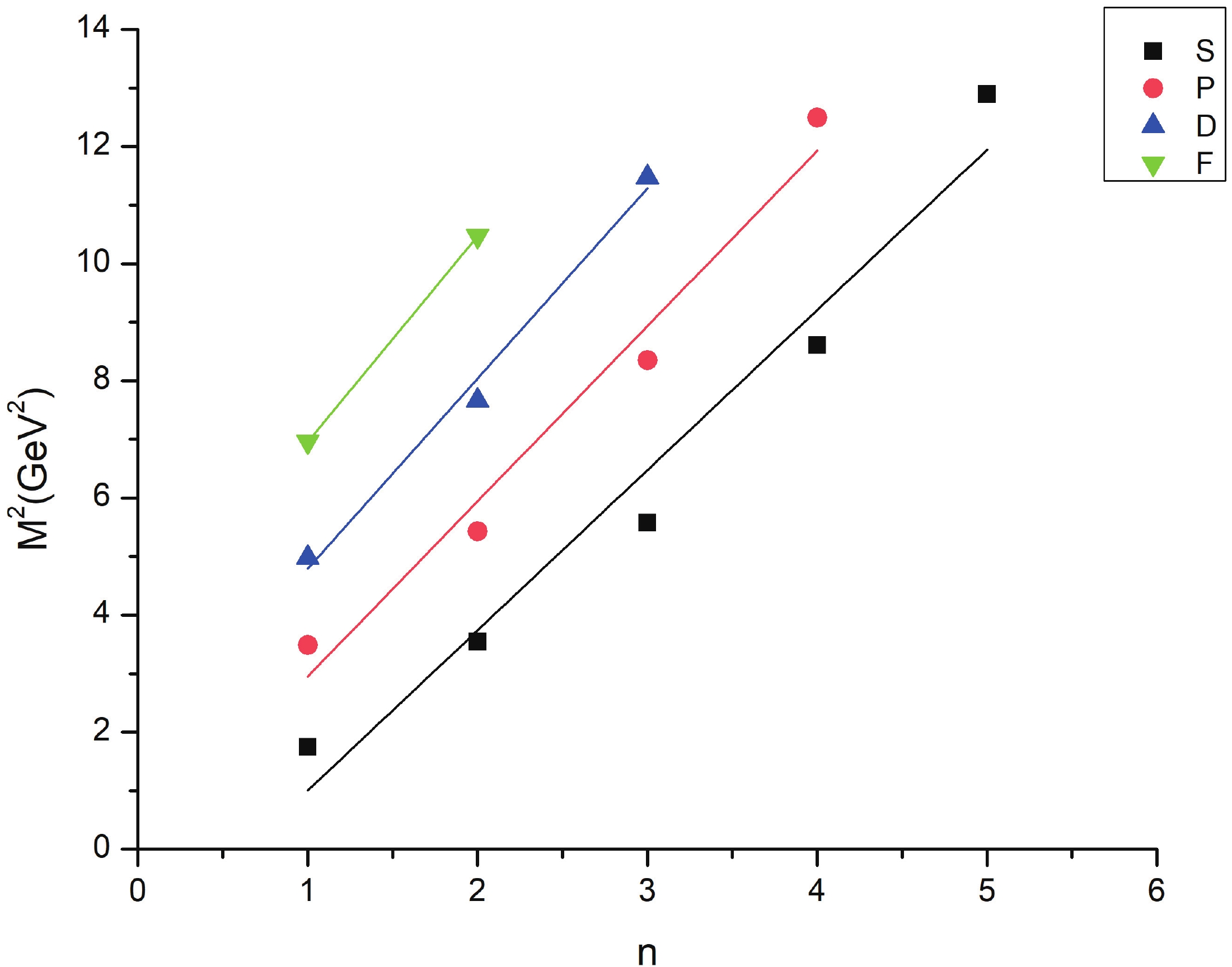
Figure 1. (color online) Regge trajectory
$ \Xi $ for$ n \rightarrow M^{2} $ 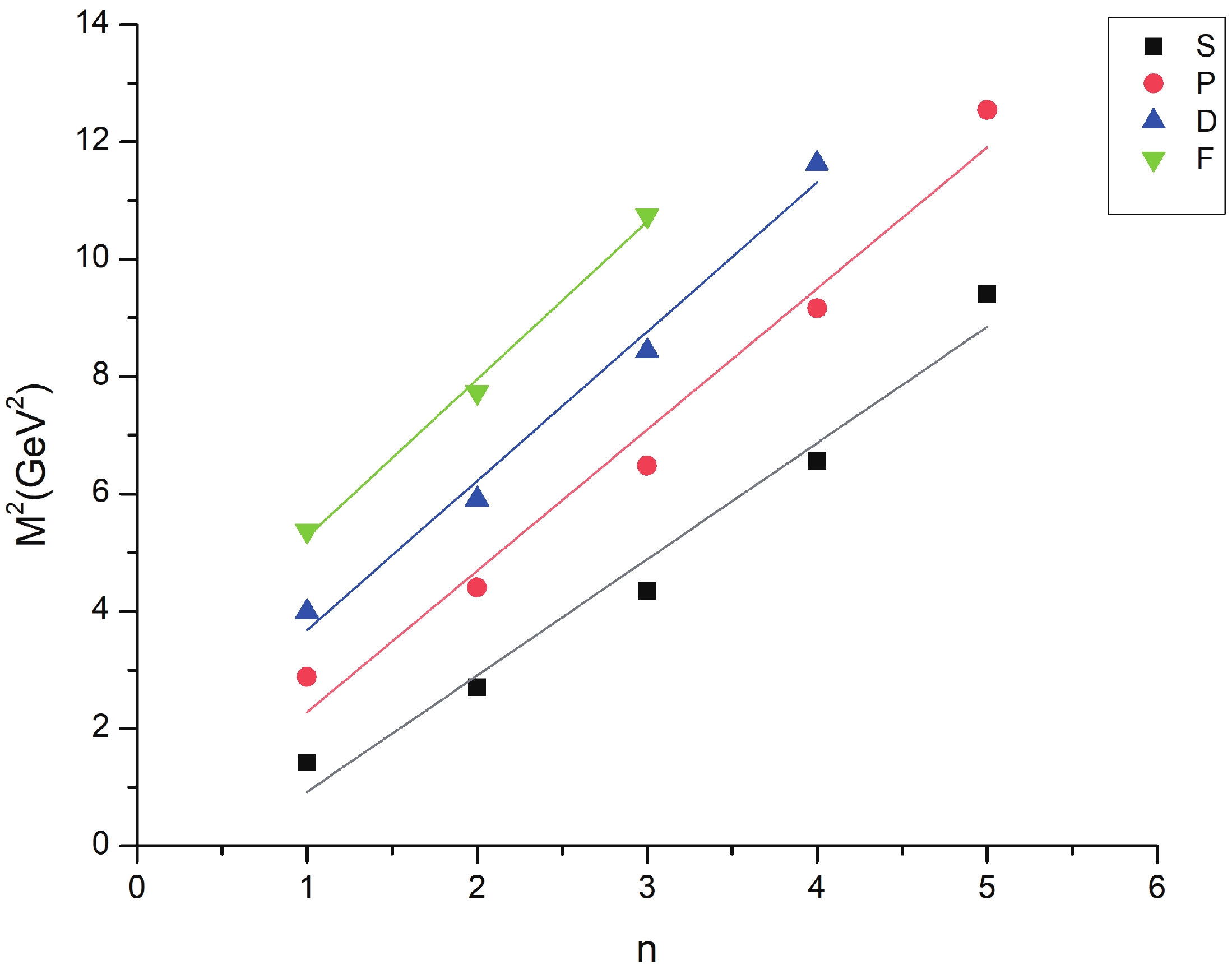
Figure 2. (color online) Regge trajectory
$ \Sigma $ for$ n \rightarrow M^{2} $ 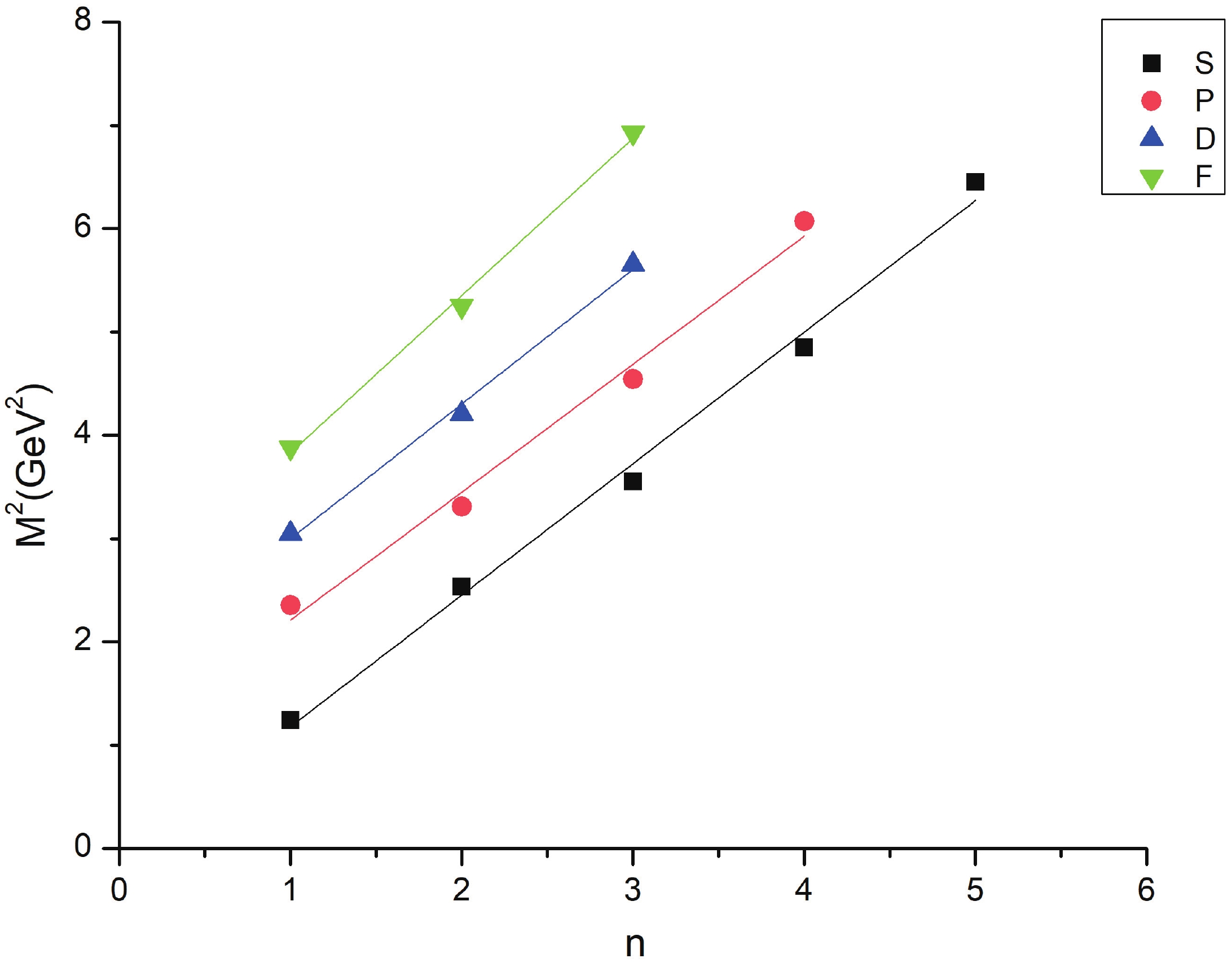
Figure 3. (color online) Regge trajectory
$ \Lambda $ for$ n \rightarrow M^{2} $ 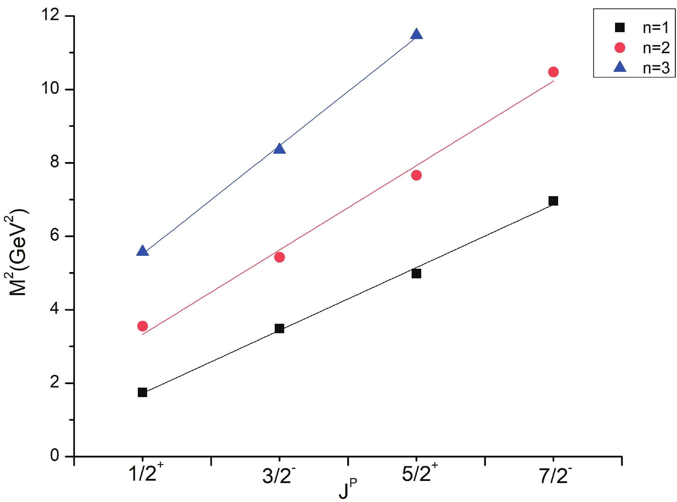
Figure 4. (color online) Regge trajectory
$ \Xi $ for$ J^{P} \rightarrow M^{2} $ 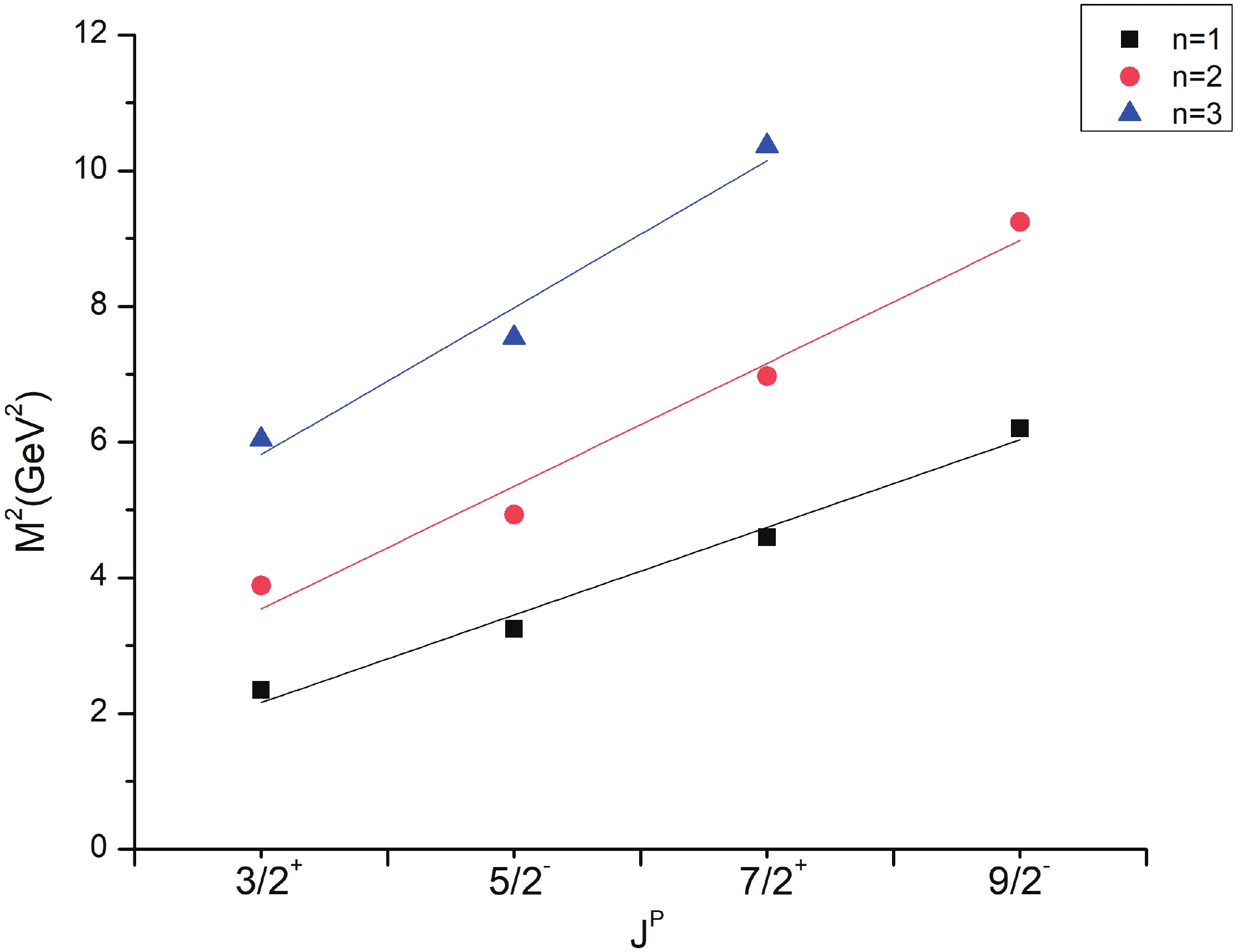
Figure 5. (color online) Regge trajectory
$ \Xi $ for$ J^{P} \rightarrow M^{2} $ 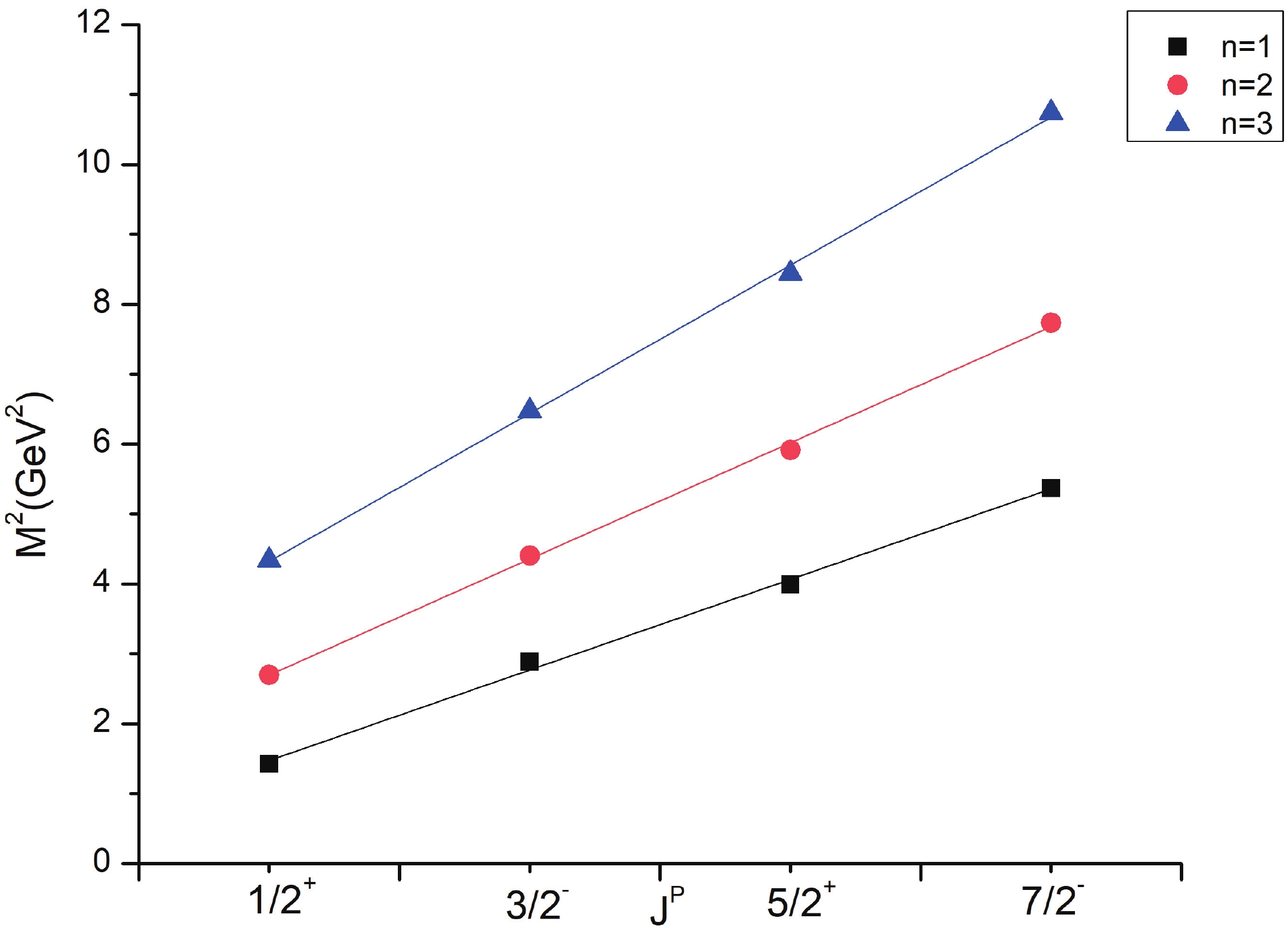
Figure 6. (color online) Regge trajectory
$ \Sigma $ for$ J^{P} \rightarrow M^{2} $ 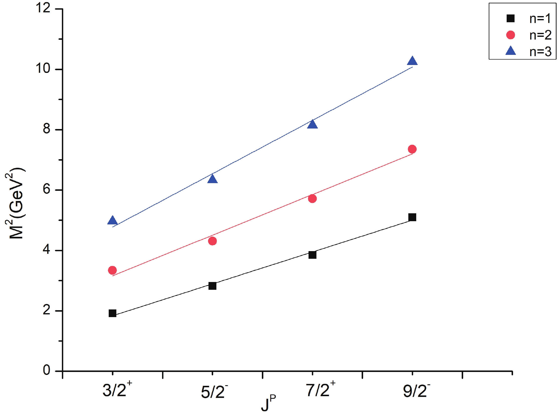
Figure 7. (color online) Regge trajectory
$ \Sigma $ for$ J^{P} \rightarrow M^{2} $ 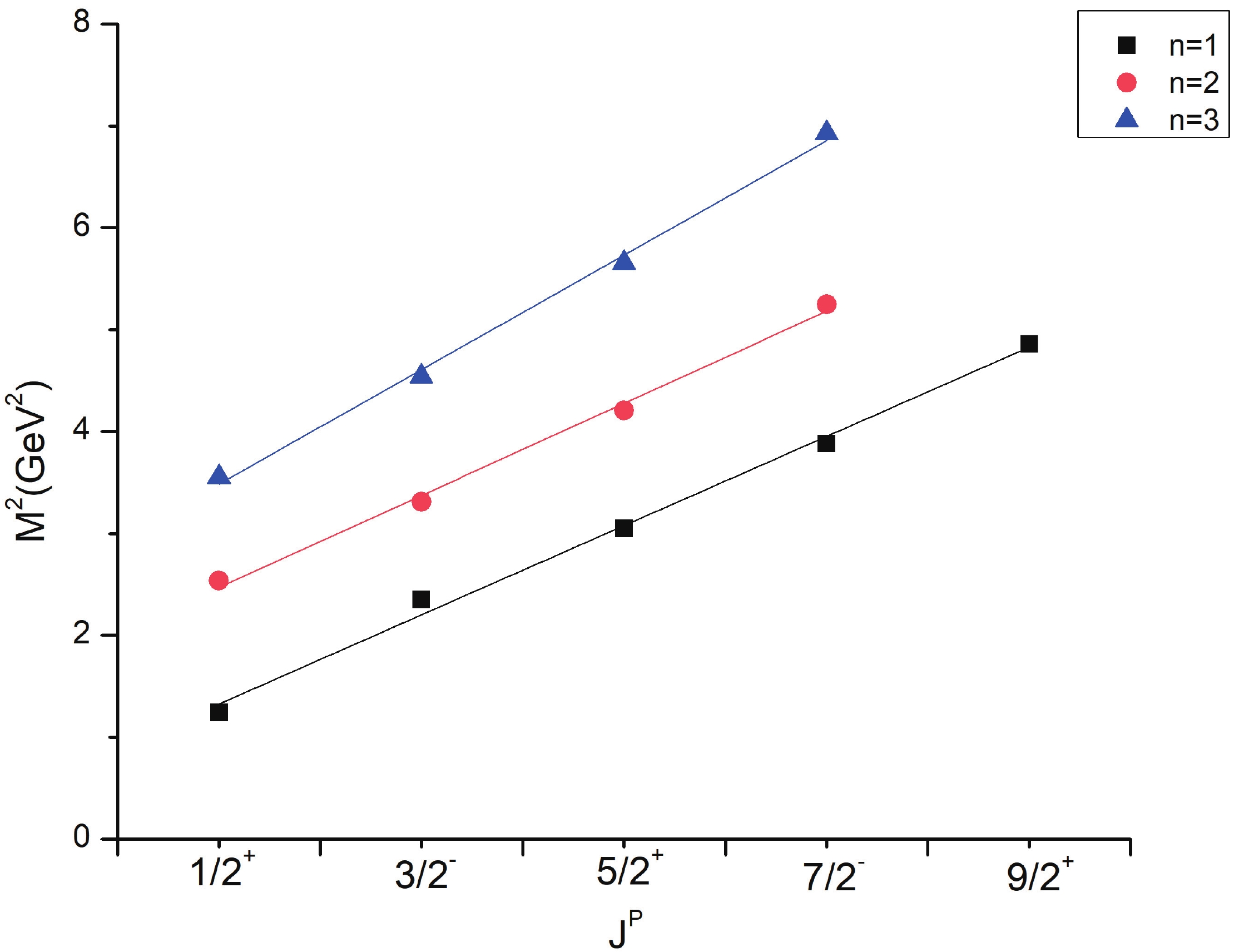
Figure 8. (color online) Regge trajectory
$ \Lambda $ for$ J^{P} \rightarrow M^{2} $ -
The study of electromagnetic properties of baryons is an active area for theoretical as well as experimental work. This intrinsic property helps reveal the shape and other dynamics of transition in decay modes. In the case of cascade
$ \Xi $ and$ \Sigma $ baryon, the magnetic moment is to be determined for both spin configurations based on the respective spin-flavor wave-function. The generalized form of the magnetic moment is$ \mu_{B} = \sum\limits_{q} \left\langle \phi_{\rm sf} \vert \mu_{qz}\vert \phi_{\rm sf} \right\rangle, $

(11) where
$ \phi_{\rm sf} $ is the spin-flavor wave function. The contribution from an individual quark appears as$ \mu_{qz} = \dfrac{e_{q}}{2m_{q}^{\rm eff}}\sigma_{qz}, $

(12) $ e_{q} $ being the quark charge,$ \sigma_{qz} $ being the spin orientation, and$ m_{q}^{\rm eff} $ is the effective mass, which may vary from model-based quark mass due to the interactions. Here, is it noteworthy that a magnetic moment shall have contributions from many other effects within the baryon such as the sea quark, valence quark, and orbital. Various models have contributed to obtaining the magnetic moment of the octet and decuplet baryons. The order of quarks in spin-flavor will not affect the magnetic moment calculation. The final spin-flavor wave function along with the calculated ground state magnetic moment in terms of the nuclear magneton ($ \mu_{N} $ ) are mentioned in Table 21.Spin Baryon $\sigma_{qz}$ 

Mass/MeV $\mu$ (

$\mu_{N}$ )

$\dfrac{1}{2}$ 

$\Xi^{0}$ (uss)

$\dfrac{1}{3}(4\mu_{s}-\mu_{u})$ 

1322 −1.50 $\dfrac{1}{2}$ 

$\Xi^{-}$ (dss)

$\dfrac{1}{3}(4\mu_{s}-\mu_{d})$ 

1322 −0.46 $\dfrac{3}{2}$ 

$\Xi^{*0}$ (uss)

$(2\mu_{s}+\mu_{u})$ 

1531 0.766 $\dfrac{3}{2}$ 

$\Xi^{*-}$ (dss)

$(2\mu_{s}+\mu_{d})$ 

1531 −1.962 $\dfrac{1}{2}$ 

$\Sigma^{+}$ (uus)

$\dfrac{1}{3}(4\mu_{u}-\mu_{s})$ 

1193 2.79 $\dfrac{1}{2}$ 

$\Sigma^{0}$ (uds)

$\dfrac{1}{3}(2\mu_{u}+2\mu_{d}-\mu_{s})$ 

1193 0.839 $\dfrac{1}{2}$ 

$\Sigma^{-}$ (dds)

$\dfrac{1}{3}(4\mu_{d}-\mu_{s})$ 

1193 −1.113 $\dfrac{3}{2}$ 

$\Sigma^{*+}$ (uus)

$(2\mu_{u}+\mu_{s})$ 

1384 2.877 $\dfrac{3}{2}$ 

$\Sigma^{*0}$ (uds)

$(\mu_{u}+\mu_{d}+\mu_{s})$ 

1384 0.353 $\dfrac{3}{2}$ 

$\Sigma^{*-}$ (dds)

$(2\mu_{d}+\mu_{s})$ 

1384 −2.171 $\dfrac{1}{2}$ 

$\Lambda^{0}$ (uds)

$\mu_{s}$ 

1115 −0.606 Table 21. Magnetic moment for ground states.
Table 22 provides a comparison of present magnetic moments with those of different approaches. H. Dahiya et al. presented octet and decuplet baryon magnetic moments in a chiral quark model with configuration mixing and generalizing the Cheng-Li mechanism. Effective mass and a screened charge scheme have been employed in Refs. [62], and both results appear in the table. Light-cone sum rules [63] and lattice QCD [64] have also been employed for octet and decuplet magnetic moments. A recent study focused on the hyperonic medium at a finite temperature using the chiral mean field approach [65]. Our results are under-predicted compared to the experimental values of PDG by 0.5 and 0.4 for
$ \Xi $ octet baryons; however, there are large variations in the case of decuplet considering all the approaches. It is expected that experimental decuplet values shall be the deciding factor. In the case of$ \Lambda^{0} $ , the magnetic moment is nearly the same as those obtained in [1], [58], and [64]. For$ \Sigma^{+} $ and$ \Sigma^{-} $ , the results are within a 0.5$ \mu_{N} $ variation for all the approaches.Baryon $\mu_{\rm cal}$ 

Exp [1] [58] [58] [59] [60, 61] [62] [62] [63] [64] [65] [66] $\Xi^{0}$ 

−1.50 −1.25 −1.41 −1.39 −1.3 −1.25 −1.37 $\Xi^{-}$ 

−0.46 −0.651 −0.50 −0.50 −0.7 −1.07 −0.82 $\Xi^{*0}$ 

0.766 0.60 0.49 0.49 0.69 0.48 0.32 0.44 0.16 0.508 0.65 $\Xi^{*-}$ 

−1.962 −2.11 −2.43 −2.27 −1.18 −1.9 −2.05 −2.27 −0.62 −1.805 −2.30 $\Sigma^{+}$ 

2.79 2.458 2.61 2.64 2.46 2.87 $\Sigma^{0}$ 

0.839 0.11 0.65 0.76 $\Sigma^{-}$ 

−1.113 −1.16 −1.01 −1.28 −1.13 −1.16 −1.48 $\Sigma^{*+}$ 

2.877 3.02 3.07 2.85 2.56 2.54 2.63 1.27 3.028 $\Sigma^{*0}$ 

0.353 0.30 0.08 0.09 0.23 0.14 0.08 0.33 0.188 $\Sigma^{*-}$ 

−2.171 −2.41 −2.92 −2.66 −2.10 −2.19 −2.43 −1.88 −2.015 $\Lambda^{0}$ 

−0.606 −0.613 −0.59 −0.60 −0.11 −0.51 −0.70 Table 22. Comparison of calculated magnetic moments with various models (All data in units of
$\mu_{N}$ ).Here, an effort has been made to determine the magnetic moment of the low-lying negative parity state of
$ \Xi $ , which was inspired by studies based on N(1535). The hyperfine interactions between the constituent quarks induce linear combinations of two states with the same angular momentum value. The magnetic moment will now have contribution from spin as well as orbital angular momentum as [67]$ \mu = \mu^{S} + \mu^{L} = \sum \dfrac{Q_{q}}{m_{q}}S_{q} + \sum \dfrac{Q_{q}}{2m_{q}}l_{q}. $

(13) The
$ J^{P} = \dfrac{1}{2}^{-} $ , L = 1 for$ S = \dfrac{1}{2} $ and$ S = \dfrac{3}{2} $ , and calculated resonance masses are 1886 and 1894 MeV, respectively. These states are not experimentally established; however, 1690 MeV is tentatively assigned by many predictions to this state. The physical eigenvalues will be$ |\Xi(1886)\rangle = {\rm cos}\theta |^{2}P_{1/2}\rangle - {\rm sin}\theta |^{4}P_{1/2}\rangle, $

(14) $ |\Xi(1894)\rangle = {\rm sin}\theta |^{2}P_{1/2}\rangle + {\rm cos}\theta |^{4}P_{1/2}\rangle. $

(15) From the approach of NCQM described in Ref. [68], we directly write the final wave-function with mixing for
$ \Xi^{0}(uss) $ as$ \left(\dfrac{2}{9}\mu_{s} + \dfrac{1}{9}\mu_{u}\right){\rm cos}^{2}\theta + \left(\mu_{s} + \dfrac{1}{3}\mu_{u}\right){\rm sin}^{2}\theta - \left(\dfrac{8}{9}\mu_{s} - \dfrac{8}{9}\mu_{u}\right){\rm cos}\theta {\rm sin}\theta. $

(16) The mixing angle is taken as
$ \theta = -31.7 $ . The magnetic moment for$ \Xi^{0}(1886) $ is obtained to be -0.695$ \mu_{N} $ , which is -0.99$ \mu_{N} $ by [68]. Similarly, for$ \Xi^{-}(1886) $ , the magnetic moment is obtained as -0.193$ \mu_{N} $ as compared to -0.315$ \mu_{N} $ [68]. The variation relies on the fact that resonance mass is model dependent and the effective mass used in the calculation ultimately depends on resonance mass. -
The transition magnetic moment as well as the radiative decay width are important in the understanding of the internal structure of baryon in addition to the magnetic and electric transitions. Many approaches have been used for the study of radiative decay over the years including some recent ones [69]. Here,
$ \Xi^{*0} \rightarrow \Xi^{0}\gamma $ and$ \Sigma^{*} \rightarrow \Sigma\gamma $ have been studied using the effective mass obtained with the hCQM approach. The generalized form for the transition magnetic moment is [70],$ \mu(B_{\frac{3}{2}^+} \rightarrow B_{\frac{1}{2}^+}) = \langle B_{\frac{1}{2}^+}, S_{z} = \dfrac{1}{2}|\mu_{z}| B_{\frac{3}{2}^+}, S_{z} = \dfrac{1}{2} \rangle. $

(17) The spin-flavor wave function is obtained similar to the above for decuplet and octet
$ \Xi $ as$ \dfrac{2\sqrt{2}}{3}(\mu_{u}^{\rm eff}-\mu_{s}^{\rm eff}). $

(18) The effective mass here is a geometric mean of those for spin
$ \dfrac{1}{2} $ and$ \dfrac{3}{2} $ . Our result comes out to be 2.378$ \mu_{N} $ , which is in good agreement with various models implemented in [62, 70]. The radiative decay width is obtained as [71]$ \Gamma_{R} = \dfrac{q^{3}}{m_{p}^{2}}\dfrac{2}{2J+1}\dfrac{e^{2}}{4\pi}\big|\mu_{\frac{3}{2}^+ \rightarrow \frac{1}{2}^+}\big|^{2}, $

(19) where q is the photon energy,
$ m_{p} $ is the proton mass, and J is the initial angular momentum giving$ \Gamma_{R} $ = 0.214 MeV. The total decay width available from the experiment is 9.1 MeV. Thus, the branching ratio$ \dfrac{\Gamma_{R}}{\Gamma_{\rm total}} $ is 2.35%, where the PDG data suggests$ <3.7 $ %. Thus, it is in accordance with other results as well as the experimental data. The radiative decay of$ \Sigma $ baryons with transition magnetic moments are summarized in Table 23. The obtained results are consistent with experimental data from PDG as well as a few other theoretical approaches.Decay Wave-function Transition moment(in $\mu_{N}$ )

$\Gamma_{R}$ (in MeV)

$\Sigma^{*0} \rightarrow \Lambda^{0}\gamma$ 

$\dfrac{\sqrt{2}}{\sqrt{3}}(\mu_{u}-\mu_{d})$ 

2.296 0.4256 $\Sigma^{*0} \rightarrow \Sigma^{0}\gamma$ 

$\dfrac{\sqrt{2}}{3}(\mu_{u}+\mu_{d}-2\mu_{s})$ 

0.923 0.0246 $\Sigma^{*+} \rightarrow \Sigma^{+}\gamma$ 

$\dfrac{2\sqrt{2}}{3}(\mu_{u}-\mu_{s})$ 

2.204 0.1404 $\Sigma^{*-} \rightarrow \Sigma^{-}\gamma$ 

$\dfrac{2\sqrt{2}}{3}(\mu_{d}-\mu_{s})$ 

−0.359 0.0037 Table 23.
$\Sigma^{*} $ Radiative decays. -
The present work aimed at studying the strangeness of -1
$ \Lambda $ and$ \Sigma $ and -2$ \Xi $ light baryon owing to the limited data on these. The non-relativistic hypercentral constituent quark model (hCQM) has been a tool for obtaining a large number of resonance masses with a linear term. The results have been compared for cases with and without first order correction terms as well, where there is a difference of a few MeV for low-lying states and up to 30 MeV for higher excited states for$ \Xi $ . The octet and decuplet states have not been exclusively distinguished due to a lack of required data.The mass-range has been compared to various theoretical approaches listed in Sec. 3. The state-wise comparison is not possible because no approach has established spin-parity assignments. The overview of Tables 6 and 7 shows that the low-lying resonance masses are in good agreement among each other especially the four star states of PDG. For higher excited states, present work overestimates the results compared to other models. The
$ \Xi $ (1820) differs by 48 MeV from the PDG mass. The$ \Xi(2030) $ state with$ J = \dfrac{5}{2} $ could find a place with either positive or negative parity as both have masses in that range.$ \Xi $ (1620) and$ \Xi $ (1690) are not obtained in present results. However,$ \Xi $ (1690), which is likely$ \dfrac{1}{2}^{-} $ as found by BABAR Collaboration, is calculated as 1886 MeV in this work. A few differences in results exist owing to the model dependent factors. As for$ \Lambda $ (1405), hCQM could not establish the mass but predicts the other negative parity state with good agreement. The four star states for$ \Sigma $ and$ \Lambda $ also agree with many approaches to a good extent.The Regge trajectories based on some resonance mass are plotted. The principal quantum number n against the square of mass
$ M^{2} $ shows a linear nature but the fitted lines are not exactly parallel. The angular momentum J versus the square of mass$ M^{2} $ plots also depict the linearity of data points, which validates our spin-parity assignments to a particular state and may be helpful in new experimental states.The magnetic moments for spin
$ \dfrac{1}{2} $ as well as$ \Xi^{0} $ and$ \Xi^{-} $ vary by 0.25$ \mu_{N} $ and 0.19$ \mu_{N} $ , respectively, from those of PDG as well as other results. For spin$ \dfrac{3}{2} $ as well as$ \Xi^{*0} $ and$ \Xi^{*-} $ , our results vary from nearly 0.2$ \mu_{N} $ to 0.4$ \mu_{N} $ compared to all approaches. The transition magnetic moment is obtained for$ \Xi^{0} $ 1886 MeV of our spectra, which differs by 0.30$ \mu_{N} $ , and$ \Xi^{-} $ differs by 0.12$ \mu_{N} $ from that in Ref. [68]. However, the difference in magnetic moment follows due to the difference in resonance masses used for the calculation. Similarly for$ \Sigma^{+} $ ,$ \Sigma^{-} $ , and$ \Lambda^{0} $ , the results are in good accordance with other approaches and PDG.The transition magnetic moment was obtained as 2.378
$ \mu_{N} $ , which agrees with other models. Moreover, the radiative decay width branching fraction was found to be 2.35% in our case, which was well within the PDG range of$ <3.7 $ %. The transition magnetic moment and radiative decay width for$ \Sigma $ were similar to other results.Thus, with some agreements and discrepancies, this work with a large number of predicted resonances along with important properties, may be helpful for upcoming experimental facilities like PANDA, which is expected to intensively study the light strange baryons [10-13, 15, 16].
-
Ms. Chandni Menapara would like to acknowledge the support from the Department of Science and Technology (DST) under the INSPIRE-FELLOWSHIP scheme for pursuing this work.
Spectroscopic investigation of light strange S = −1 Λ and Σ and S = −2 Ξ baryons
- Received Date: 2021-02-10
- Available Online: 2021-06-15
Abstract: The present study is dedicated to light-strange


 DownLoad: