


 Abstract
 HTML
HTML Reference
 Related
 PDF
PDF


-
Despite the discovery of the Higgs boson, the standard model (SM) is generally considered a low-energy effective theory of a more fundamental one, because SM cannot elucidate the matter-antimatter asymmetry in the universe, it is not a dark matter candidate, and it does not explain its own gauge group structure. Therefore, one of the most important tasks in the particle physics community is searching for new physics (NP) beyond SM, which can be examined by probing for NP signals directly at higher energy colliders or determining the discrepancy between SM predictions and the precise data at high intensity machines indirectly. Regarding the indirect approaches, the flavor-changing neutral-current (FCNC) processes are generally considered to be an ideal plate in the determination of NP, because FCNC only occurs by loops in SM, and the corresponding branching fractions can be enhanced by new particles. However, recently, a few unexpected anomalies have been discovered in the semi-leptonic B decays induced by the charged currents
$ b\to c\ell\bar\nu_\ell $ ($ \ell = e, \mu, \tau $ ), relative to the corresponding SM predictions at the$ (2-3)\sigma $ level (see e.g. [1-5]). It exceeds our expectations to find such large deviations from SM in these processes that occur at the tree level. It should be emphasized that some anomalies might imply that the lepton flavour universality (LFU) is violated, which is hints on the existence of NP, because LFU is not considered in SM. If these measurements can be further confirmed in future experiments, they would be regarded as the distinct signals of NP. Therefore, several NP models involving new particles have been proposed to elucidate such tensions, such as$ W^\prime $ models [6-8], leptoquark models [9-12], and models with charged Higgs [13-16].Because these anomalies were initially determined in B decays, it is natural for us to investigate whether the similar discrepancy can appear in charmed meson decays induced by charged currents
$ c\to (s,d)\ell^+\nu_\ell $ ($ \ell = e, \mu, \tau $ ), and whether the newly introduced particles in the proposed models can affect the observables in D meson decays [17-19]. Although significant efforts have been devoted to determine the contributions of NP in the charm sector in the past few years [20-23], a similar anomaly has not been observed in experiments to date [24]. In the theoretical calculations, the most important inputs are the heavy-to-light form factors, which are nonpertubative and can only be calculated in some nonpertubative approaches, such as approaches based on quark models, QCD sum rules, and lattice QCD (LQCD). In particular, the predictions from LQCD are more preferred, as LQCD is based on the first principles. Recently, the SM predictions of the semileptonic decays based on LQCD [25] are in agreement with the world average experimental measurements [26] with large uncertainties from the CKM matrix elements. These consistencies can be harnessed to constrain the parameter spaces of NP [27] or test NP models. In addition, except for the absolute branching fractions, most of the other observables such as the differential widths, forward-backward asymmetries, and longitudinal polarizations of the final state vector mesons, as well as the helicity asymmetries of leptons, have not been measured until now. In this study, we attempt to fit the parameters of NP with existing experimental data under a single operator assumption and further verify whether these fitted parameters contribute to the above mentioned observables. The comparisons between our results and future experimental data would be helpful in probing the effects of NP.To achieve the above purposes, we shall analyze all D meson decays induced by
$ c\to (s,d)\ell^+\nu_\ell $ in the model-independence manner, including the leptonic and semi-leptonic decays. Based on the general framework of the four-fermion effective theory, we will perform a least$ \chi^2 $ fit of the Wilson coefficient for each operator to the latest experimental data. With these obtained Wilson coefficients, we will present the predictions of other observables. For the pure leptonic D decays, we will also study LFU with existing experimental data.This paper is organized as follows. In Sec. II, the framework of this work is presented, including the effective Hamiltonian, form factors, and helicity amplitudes. We present the parameters in Sec. III. In Sec. IV, we investigate the numerical analysis of leptonic decays. The results and discussions on the semi-leptonic decays of D mesons are presented in Sec. V, and the predictions of the physical observables are also provided in this section. Finally, we conclude this work in Sec. VI.
-
In particular, the energy scale of NP is supposed to be significantly higher than the electroweak scale; thus, the operator product expansion (OPE) is often adopted in separating the long- and short-distance interactions. In OPE, the heavier degrees of freedom can be integrated out, resulting in an effective Lagrangian where all high energy physics effects are absorbed into Wilson coefficients, and the low energy physics is elucidated by the effective operators. Accordingly, considering all possible Lorentz structures and assuming neutrinos to be left-handed, we express the effective Lagrangian for the decay
$ c \to q \ell^+\nu_\ell $ (with$ q = d, s $ and$ \ell = e,\mu, \tau $ ) as [28,29]$ \begin{aligned}[b] {\cal L}_{\rm eff} =& -\frac{4G_{F}}{\sqrt{2}}V_{cq}^*\Big[(1+C^{\ell}_{VL})O^{\ell}_{VL}+C^{\ell}_{VR}O^{\ell}_{VR} +C^{\ell}_{SL}O^{\ell}_{SL} \\&+C^{\ell}_{SR}O^{\ell}_{SR}+C^{\ell}_{T}O^{\ell}_{T}\Big]+{\rm h.c.}, \end{aligned} $

(1) where
$ G_{F} $ and$ V_{cq} $ represent the Fermi constant and CKM matrix element, respectively. The four-fermion operators can be defined as$ \begin{aligned}[b] O^{\ell}_{VL} =& (\bar q\gamma^{\mu}P_{L}c)(\bar \nu_{\ell}\gamma_{\mu}P_{L}\ell), \,\, O^{\ell}_{VR} = (\bar q\gamma^{\mu}P_{R}c)(\bar \nu_{\ell}\gamma_{\mu}P_{L}\ell),\\ O^{\ell}_{SL} =& (\bar qP_{L}c)(\bar \nu_{\ell} P_{R}\ell), \,\, O^{\ell}_{SR} = (\bar qP_{R}c)(\bar \nu_{\ell} P_{R}\ell),\\ O^{\ell}_{T} =& (\bar q\sigma^{\mu\nu}P_{L}c)(\bar \nu_{\ell}\sigma_{\mu\nu}P_{L}\ell), \end{aligned} $

(2) where
$ P_{L(R)} = (1\mp\gamma^{5})/2 $ and$ C^{\ell}_{i} $ ($ i = VL,VR,SL,SR, $ and T) denote the corresponding Wilson coefficients at the scale$ \mu = m_c $ , with$ C_{i} ^{\ell} = 0 $ in SM. It should be noted that all Wilson coefficients are assumed to be real (except where specially noted) for simplicity. In other words, the NP effects do not involve new sources of CP violation. In general, the difference between$ C^\ell_{d,i} $ and$ C^\ell_{s,i} $ should be discussed. However, we paid significant attention to the violation of lepton flavour universality in this work; therefore, we neglected the difference between s and d quarks to reduce the number of new parameters as possible, namely$ C_{d,i}^\ell = C_{s,i}^\ell $ . -
In our calculations, the hadronic transitions are parameterized by the heavy-to-light form factors, which are nonperturbative and universal. For the hadronic matrix elements of
$ D\to P $ transitions, with P denoting the pseudoscalar meson, they can be defined as$ \begin{aligned}[b] \langle P(p_{2})|\bar q\gamma^{\mu}c|D(p_{1})\rangle =& f_+(q^2)\Bigg[(p_{1}+p_{2})^{\mu}-\frac{m_{D}^{2}-m_{P}^{2}}{q^{2}}q^{\mu}\Bigg] \\&+f_{0}(q^2)\frac{m_{D}^{2}-m_{P}^{2}}{q^{2}}q^{\mu}, \end{aligned} $

(3) $ \begin{aligned}[b] \langle P(p_{2})|\bar qc|D(p_{1})\rangle =& \frac{q_{\mu}}{m_{c}-m_{q}}\langle P(p_{2})|\bar q\gamma^{\mu}c|D(p_{1})\rangle \\=& \frac{m_{D}^{2}-m_{P}^{2}}{m_{c}-m_{q}}f_{0}(q^2), \end{aligned} $

(4) $ \langle P(p_{2})|\bar q \sigma^{\mu\nu} c|D(p_{1})\rangle = -{\rm i}(p^{\mu}_{1}p^{\nu}_{2}-p^{\nu}_{1}p^{\mu}_{2})\frac{2f_{T}(q^2)}{m_{D}+m_{P}}, $

(5) where
$ q^{\mu} = (p_{1}-p_{2})^{\mu} $ and the two QCD form factors,$ f_{+}(q^2) $ and$ f_{0}(q^2),$ encode the strong-interaction dynamics and satisfy$ f_{+}(0) = f_{0}(0) $ . In addition,$ m_{q} $ represents the running quark mass. Regarding the various form factors in the$ D\to K $ transitions, we adopt the latest results from the LQCD [30,31], and each form factor can be expressed as$ f_+^{D\to K}(q^{2}) = \frac{f^{D\to K}(0)+c_+^{D\to K}(z-z_{0})\left(1+\dfrac{z+z_{0}}{2}\right)}{1-q^{2}/M_{D_{s}^{*}}}^2, $

(6) $ f_{0}^{D\to K}(q^{2}) = f^{D\to K}(0)+c_{0}^{D\to K}(z-z_{0})\left(1+\frac{z+z_{0}}{2}\right), $

(7) $ f_{T}^{D\to K}(q^{2}) = \frac{f_{T}^{D\to K}(0)+c_{T}^{D\to K}(z-z_{0})\left(1+\dfrac{z+z_{0}}{2}\right)}{1-P_{T}^{D\to K}q^{2}}, $

(8) where z is defined as
$ z = \frac{\sqrt{t_+-q^{2}}-\sqrt{t_+-t_{0}}}{\sqrt{t_+-q^{2}}+\sqrt{t_+-t_{0}}}, $

(9) with
$ t_{+} $ and$ t_0 $ given by$ \begin{array}{l} t_+ = (m_{D}+m_{K})^{2},\,\,\,t_{0} = (m_{D}+m_{K})(\sqrt{m_{D}}-\sqrt{m_{K}})^{2}, \end{array} $

(10) and
$ z_0 = z(q^2 = 0) $ . For the$ D\to \pi $ transition, the scalar, vector, and tensor form factors are also parameterized as [30,31]$ f_+^{D\to \pi}(q^{2}) = \frac{f^{D\to \pi}(0)+c_+^{D\to \pi}(z-z_{0})\left(1+\dfrac{z+z_{0}}{2}\right)}{1-P_Vq^{2}}, $

(11) $ f_{0}^{D\to \pi}(q^{2}) = \frac{f^{D\to \pi}(0)+c_+^{D\to \pi}(z-z_{0})\left(1+\dfrac{z+z_{0}}{2}\right)}{1-P_Sq^{2}}, $

(12) $ f_{T}^{D\to \pi}(q^{2}) = \frac{f_{T}^{D\to \pi}(0)+c_{T}^{D\to \pi}(z-z_{0})\left(1+\dfrac{z+z_{0}}{2}\right)}{1-P_{T}^{D\to \pi}q^{2}}. $

(13) The values of all parameters are presented in Tables 1 and 2.
Decay $ f(0) $ 

$ c_+ $ 

$ P_V $ /GeV

$ ^{-2} $ 

$ c_0 $ 

$ P_S $ /GeV

$ ^{-2} $ 

$ D\rightarrow \pi $ 

0.6117 (354) −1.985 (347) 0.1314 (127) −1.188 (256) 0.0342 (122) $ D\rightarrow K $ 

0.7647 (308) −0.066 (333) − −2.084 (283) − Table 1. Parameters for
$ f_0 $ ,$ f_+ $ in the z-series expansion [30].Decay $ f_T(0) $ 

$ c_T $ 

$ P_T $ /GeV

$ ^{-2} $ 

$ D\rightarrow \pi $ 

0.5063 (786) −1.10 (1.03) 0.1461 (681) $ D\rightarrow K $ 

0.6871 (542) −2.86 (1.46) 0.0854 (671) Table 2. Parameters for
$ f_T $ in the z-series expansion [31].However, for the form factors of
$ D_s\to K $ ,$ D \to \eta^{(\prime)},$ and$ D_s\to \eta^{(\prime)} $ , LQCD results are still unavailable till now, and we have to employ the results obtained from other approaches. In this work, we adopted the results from Ref. [32], based on the light-cone sum rules. To describe the behavior of the form factors in the entire kinematically accessible region, we adopted the double-pole parametrization:$ F^i(q^{2}) = \frac{F^i(0)}{1-a\dfrac{q^{2}}{m_{D}^{2}}+b\left(\dfrac{q^{2}}{m_{D}^{2}}\right)^2}, $

(14) where
$ F^i(q^{2}) $ can be any of the form factors$ f_i $ ($ i = +,0,T $ ). For$ \eta $ and$ \eta^\prime $ , we considered mixing the light and s-quark components. The quark components are given as$ \left ( \begin{array}{cc} \eta \\ \eta^\prime \\ \end{array} \right ) = \left ( \begin{array}{cc} \sin \theta_p & \cos \theta_p \\ -\cos \theta_p & \sin \theta_p \\ \end{array} \right ) \left ( \begin{array}{cc} q\bar q \\ s\bar s \\ \end{array} \right ),\,\,\,\, q\bar q = \frac{ u\bar u + d\bar d }{\sqrt 2}. $

(15) We adopted the value
$ \theta = (39.3\pm1.0)^\circ $ from Ref. [33], and the possible gluonic contribution was neglected. The explicit values of these form factors are presented in Table 3.Decay $ F(0) $ 

$ a_F $ 

$ b_F $ 

$ D_s \rightarrow K $ 

$ f_+ $ 

$ 0.82^{+0.08}_{-0.07} $ 

$ 1.11^{-0.04}_{+0.07} $ 

$ 0.49^{-0.05}_{+0.06} $ 

$ f_0 $ 

$ 0.82^{+0.08}_{-0.07} $ 

$ 0.53^{-0.03}_{+0.04} $ 

$ -0.07^{-0.04}_{+0.04} $ 

$ D \rightarrow \eta_q $ 

$ f_+ $ 

$ 0.56^{+0.06}_{-0.05} $ 

$ 1.25^{-0.04}_{+0.05} $ 

$ 0.42^{-0.06}_{+0.05} $ 

$ f_0 $ 

$ 0.56^{+0.06}_{-0.05} $ 

$ 0.65^{-0.01}_{+0.02} $ 

$ -0.22^{-0.03}_{+0.02} $ 

$ D_s \rightarrow \eta_s $ 

$ f_+ $ 

$ 0.61^{+0.06}_{-0.05} $ 

$ 1.20^{-0.02}_{+0.03} $ 

$ 0.38^{-0.01}_{+0.01} $ 

$ f_0 $ 

$ 0.61^{+0.06}_{-0.05} $ 

$ 0.64^{-0.01}_{+0.02} $ 

$ -0.18^{+0.04}_{-0.03} $ 

Table 3. Form factors of
$ D_s\to K $ ,$ D\to \eta_q $ and$ D\to \eta_s $ [32].The hadronic matrix elements of the vector, scalar, and tensor currents between D and V (
$ V = K^{*} $ ,$ \phi $ ,$ \rho $ and$ \omega $ ) can also be parameterized into eight form factors, respectively,$ \langle V(p_{2},\varepsilon^*)|\bar q\gamma^{\mu}c|D (p_{1})\rangle = \frac{-2iV(q^2)}{m_{D}+m_{V}}\epsilon^{\mu\nu\alpha\beta}\varepsilon^*_{\nu}p_{1 \alpha}p_{2 \beta}, $

(16) $ \begin{aligned}[b] \langle V(p_{2},\varepsilon^*)|\bar q\gamma^{\mu}\gamma_{5} c|D(p_{1})\rangle =& -(m_{D}+m_{V})\varepsilon^{*\mu}A_{1}(q^2)\\&+\frac{\varepsilon^{*}\cdot q}{m_{D }+m_{V}}(p_{1}+p_{2})^{\mu}A_{2}(q^2)\\ & +2m_{V}\frac{\varepsilon^{*}\cdot q}{q^{2}}q^{\mu}\left(A_{3}(q^2)-A_{0}(q^2)\right), \end{aligned} $

(17) $ \begin{aligned}[b] \langle V(p_{2},\varepsilon^*)|\bar q\sigma^{\mu\nu}c|D (p_{1})\rangle =& \epsilon^{\mu\nu\rho\sigma}\Bigg[\varepsilon_{\rho}^{*}(p_{1}+p_{2})_{\sigma}T_{1}(q^2)\\&+ \varepsilon_{\rho}^{*}q_{\sigma}\frac{m_{D}^{2}-m_{V}^{2}}{q^{2}}(T_{2}(q^2)-T_{1}(q^2))\\ & +2\frac{\varepsilon^{*}\cdot q}{q^{2}}p_{1\rho}p_{2\sigma}(T_{2}(q^2)\\&-T_{1}(q^2)+\frac{q^{2}}{m_{D}^{2}-m_{V}^{2}}T_{3}(q^2))\Bigg], \end{aligned} $

(18) where
$ A_{0} $ is defined as$ \begin{aligned}[b] A_{0}(q^2) =& \frac{1}{2m_{V}}\Big[(m_{D}+m_{V})A_{1}(q^2)\\&-(m_{D}-m_{V})A_{2}(q^2) -\frac{q^2}{m_{D}+m_{V}}A_{3}(q^2)\Big]. \end{aligned} $

(19) For the form factors of
$ D \to V $ , there are several studies in literature based on different approaches, such as QCD sum rules [34], light-cone sum rules (LCSR) [32,35,36], quark models [37-43], covariant light-front quark models [44,45], and LQCD [46,47]. The results of$ D \to K^*, \rho $ from LQCD had been released in as early as 1995 [46]; however, the predicted branching fraction of$ D^+ \to K^{*+}\mu \nu_\mu $ is significantly larger than the upper limits of experimental result [48]. The recent undated results from LQCD remain absent to date. In 2013, the HPQCD collaboration calculated the complete set of axial and vector form factors of$ D_s^+ \to \phi $ [47]; however, the ratios at the maximum recoil of$ A_2(0)/A_1(0) $ and$ V(0)/A_1(0) $ are smaller than the experimental data [38]. The form factors$ D_s^+ \to K^{*} $ and$ D \to \omega $ have not been explored in LQCD till now. Although most results [44] of the covariant light-front quark model agree well with the experimental data [26] with certain uncertainties, the predicted branching fraction of$ D \to K^*\mu^+\nu_\mu $ is also significantly larger than the experimental data, which reduces its prediction power. Regarding other results based on quark models, a comprehensive study involving all$ D \to V $ processes of all possible currents does not exist, to the best of our knowledge. For consistency, we adopted the results with the LCSR calculation of Ref. [32], which is based on the framework of the heavy quark effective field theory. Although this work dates back to 2006, a few recent determinations exist [35,36]. In our calculations, the double-pole parametrization expressed in Eq. (14) was also selected to interpolate the calculated values of the form factors, and here,$ F^i $ was any of the form factors$ A_1 $ ,$ A_2 $ ,$ A_3,$ and V. The values of the parameters are presented in Table 4. In the heavy quark effective theory, the tensor form factors of$ D \to V $ are related to the vector and scalar form factors$ A_1 $ ,$ A_2 $ ,$ A_3,$ and V, and their relationships are given as$ \hspace{1.15cm}F\hspace{1.15cm} $ 

$ \hspace{1.15cm}a\hspace{1.15cm} $ 

$ \hspace{1.15cm}b\hspace{1.15cm} $ 

$ A_{1}^{D \to K^{*}} $ 

$ 0.571^{+0.020}_{-0.022} $ 

$ 0.65^{-0.06}_{+0.10} $ 

$ 0.66^{-0.18}_{+0.21} $ 

$ A_{2}^{D \to K^{*}} $ 

$ 0.345^{+0.034}_{-0.037} $ 

$ 1.86^{+0.05}_{-0.22} $ 

$ -0.91^{+0.48}_{-0.97} $ 

$ A_{3}^{D \to K^{*}} $ 

$ -0.723^{+0.065}_{-0.077} $ 

$ 1.32^{+0.14}_{-0.09} $ 

$ 1.28^{+0.22}_{-0.21} $ 

$ V^{D \to K^{*}} $ 

$ 0.791^{+0.024}_{-0.026} $ 

$ 1.04^{-0.17}_{+0.25} $ 

$ 2.21^{-0.12}_{+0.37} $ 

$ A_{1}^{D_{s} \to K^{*}} $ 

$ 0.589^{+0.040}_{-0.042} $ 

$ 0.56^{-0.02}_{+0.02} $ 

$ -0.12^{+0.03}_{-0.02} $ 

$ A_{2}^{D_{s} \to K^{*}} $ 

$ 0.315^{+0.024}_{-0.018} $ 

$ 0.15^{+0.22}_{-0.14} $ 

$ 0.24^{-0.94}_{+0.83} $ 

$ A_{3}^{D_{s} \to K^{*}} $ 

$ -0.675^{+0.027}_{-0.037} $ 

$ 0.48^{-0.11}_{+0.13} $ 

$ -0.14^{+0.18}_{-0.17} $ 

$ V^{D_{s} \to K^{*}} $ 

$ 0.771^{+0.049}_{-0.049} $ 

$ 1.08^{-0.02}_{+0.02} $ 

$ 0.13^{-0.03}_{-0.02} $ 

$ A_{1}^{D_{s} \to \phi} $ 

$ 0.569^{+0.046}_{-0.049} $ 

$ 0.84^{-0.05}_{+0.06} $ 

$ 0.16^{-0.01}_{+0.01} $ 

$ A_{2}^{D_{s} \to \phi} $ 

$ 0.304^{+0.021}_{-0.017} $ 

$ 0.24^{+0.18}_{-0.05} $ 

$ 1.25^{-1.08}_{+1.02} $ 

$ A_{3}^{D_{s} \to \phi} $ 

$ -0.757^{+0.029}_{-0.039} $ 

$ 0.60^{-0.02}_{+0.07} $ 

$ 0.60^{+0.31}_{-0.33} $ 

$ V^{D_{s} \to \phi} $ 

$ 0.778^{+0.057}_{-0.062} $ 

$ 1.37^{-0.05}_{+0.04} $ 

$ 0.52^{+0.04}_{-0.06} $ 

$ A_{1}^{D\to \rho} $ 

$ 0.599^{+0.035}_{-0.030} $ 

$ 0.44^{-0.06}_{+0.10} $ 

$ 0.58^{-0.04}_{+0.23} $ 

$ A_{2}^{D\to \rho} $ 

$ 0.372^{+0.026}_{-0.031} $ 

$ 1.64^{-0.16}_{+0.10} $ 

$ 0.56^{-0.28}_{+0.04} $ 

$ A_{3}^{D\to \rho} $ 

$ -0.719^{+0.055}_{-0.066} $ 

$ 1.05^{+0.15}_{-0.15} $ 

$ 1.77^{-0.11}_{+0.20} $ 

$ V^{ D\to \rho} $ 

$ 0.801^{+0.044}_{-0.036} $ 

$ 0.78^{-0.20}_{+0.24} $ 

$ 2.61^{+0.29}_{-0.04} $ 

$ A_{1}^{D\to \omega } $ 

$ 0.556^{+0.033}_{-0.028} $ 

$ 0.45^{-0.05}_{+0.09} $ 

$ 0.54^{-0.10}_{+0.17} $ 

$ A_{2}^{D\to \omega } $ 

$ 0.333^{+0.026}_{-0.030} $ 

$ 1.67^{-0.15}_{+0.09} $ 

$ 0.44^{-0.29}_{+0.05} $ 

$ A_{3}^{D\to \omega } $ 

$ -0.657^{+0.053}_{-0.063} $ 

$ 1.07^{+0.17}_{-0.14} $ 

$ 1.77^{+0.14}_{+0.07} $ 

$ V^{ D\to \omega } $ 

$ 0.742^{+0.041}_{-0.034} $ 

$ 0.79^{-0.20}_{+0.22} $ 

$ 2.52^{+0.28}_{-0.13} $ 

Table 4. Form factor of
$ D(D_{s})\to V $ transitions obtained in the LCSR [32].$ T_1(q^2) = \frac{m_D^2 - m_V^2 + q^2}{2 m_D} \frac{V(q^2)}{m_D + m_V} + \frac{m_D + m_V}{2 m_D} A_1(q^2) , $

(20) $ \begin{aligned}[b] T_2(q^2) =& \frac{2}{m_D^2 - m_V^2} \Bigg[ \frac{(m_D - y)(m_D + m_V)}{2} A_1(q^2)\\&+ \frac{m_D (y^2 - m_V^2)}{m_D + m_V} V(q^2) \Bigg] , \end{aligned} $

(21) $ \begin{aligned}[b] T_3(q^2) =& -\frac{m_D + m_V}{2 m_D} A_1(q^2) + \frac{m_D - m_V}{2 m_D} \big[ A_2(q^2) - A_3(q^2)\big]\\& + \frac{m_D^2 + 3 m_V^2 - q^2}{2 m_D (m_D + m_V)} V(q^2), \end{aligned} $

(22) where the energy y of the final vector meson is given by
$ y = \frac{m_D^2 + m_V^2 - q^2}{2 m_D}. $

(23) -
In SM, the transitions
$ c\to s\ell^+ \nu_\ell $ can be viewed as subsequent processes$ c\to sW^{*+} $ and$ W^{*+}\to \ell^+ \nu_\ell $ . It is well known that the off-shell$ W^{*+} $ has four helicities, including$ \lambda_{W} = \pm1,0 $ ($ J = 1 $ ) and$ \lambda_{W} = 0 $ ($ J = 0 $ ), and only the$ W^{*+} $ boson has a timelike polarization, with$ J = 1,0 $ , thus denoting the two angular momenta in the rest frame of the$ W^{*} $ boson. To distinguish the two$ \lambda_{W} = 0 $ states, we set$ \lambda_{W} = 0 $ for$ J = 1 $ and$ \lambda_{W} = t $ for$ J = 0 $ . In the D meson rest frame, we set the z-axis to be along the moving direction of$ W^{*+} $ , and its polarization vectors are expressed as$ \begin{aligned}[b] \epsilon^{\mu}(\pm) =& \frac{1}{2}(0,1,\mp i,0),\\\epsilon^{\mu}(0) =& -\frac{1}{\sqrt{q^{2}}}(q_{3},0,0,q_{0}),\\\epsilon^{\mu}(t) =& -\frac{q^{\mu}}{\sqrt{q^{2}}}, \end{aligned} $

(24) where
$ q^{\mu} $ is the four-momentum of the$ W^{*+} $ . The polarization vectors of the virtual$ W^{*+} $ satisfy the orthogonality and completeness relationship:$ \begin{array}{l} \epsilon^{*\mu}(m)\epsilon_{\mu}(n) = g_{mn},\,\,\,\sum_{m,n}\epsilon^{*\mu}(m)\epsilon^{\nu}(n)g_{mn} = g^{\mu\nu}, \end{array} $

(25) where
$ g_{mn} $ is diag ($ +,-,-,- $ ) for$ m,n = t,\pm,0 $ .In the calculations, the total matrix element can be factorized into leptonic and hadronic parts, both of which are not the Lorentz invariant. Both parts become Lorentz invariant after contracting with the polarization vector of
$ W^{*+} $ , which allows us to select the coordinate system arbitrarily. Thereby, the hadron side can be analyzed in the initial state D meson rest frame, and the lepton side will be analyzed in the virtual$ W^{*+} $ rest frame. We then calculate the helicity amplitudes of the$ D\to PW^{*+} $ transition as$ H^{PV}_{\lambda_{W}}(q^{2}) = \epsilon^{*}_{\mu}(\lambda_{W})\langle P(p_{2})|\bar q\gamma^{\mu}c|D(p_{1})\rangle, $

(26) $ H^{PS}(q^{2}) = \langle P(p_{2})|\bar qc|D(p_{1})\rangle, $

(27) $ H^{PT}_{\lambda_{W},\lambda_{W}^{\prime}}(q^{2}) = \epsilon^{*}_{\mu}(\lambda_{W})\epsilon^{*}_{\nu}(\lambda_{W}^{\prime}) \langle P(p_{2})|\bar q\sigma^{\mu\nu}c|D(p_{1})\rangle. $

(28) Similarly, the helicity amplitudes of the
$ D\to VW^{*+} $ transition are given as$ \begin{aligned}[b] H^{VAL(VAR)}_{\lambda_{W},\varepsilon_{V}}(q^{2}) =& \epsilon^{*}_{\mu}(\lambda_{W}) \langle V(p_{2},\varepsilon^*)|\bar q\gamma^{\mu}(1\pm\gamma^{5})c|D_{(s)}(p_{1})\rangle,\\ H^{SPL(SPR)}_{\varepsilon_{V}}(q^{2}) =& \langle V(p_{2},\varepsilon^*)|\bar q\gamma^{\mu}(1\pm\gamma^{5})c|D_{(s)}(p_{1})\rangle,\\ H^{T}_{\lambda_{W},\lambda_{W}^{'},\varepsilon_{V}}(q^{2}) =& \epsilon^{*}_{\mu}(\lambda_{W}) \epsilon^{*}_{\nu}(\lambda_{W}^{'})\langle V(p_{2},\varepsilon^*)\\&\times |\bar q\sigma^{\mu\nu} (1-\gamma^{5})c|D_{(s)}(p_{1})\rangle. \end{aligned} $

(29) For an arbitrary decay
$ D\to F \ell^+\nu_\ell $ ($ F = P,V $ ), owing to the conservation of helicity,$ -\varepsilon_{F} + \lambda_{W^*} = 0 $ is satisfied,$ \varepsilon_{F} $ being the polarization of the final state F. Therefore, only five helicity amplitudes contribute to$ D\to P\ell^+\nu_\ell $ decays, which are given as$ \begin{aligned}[b]& H^{PV}_{0} = \frac{f_+\sqrt{Q_+Q_-}}{\sqrt{q^2}}\,, H^{PV}_{t} = \frac{f_{0}M_+M_-}{\sqrt{q^2}}\,, H^{PS} = \frac{f_{0}M_+M_-}{m_{c}-m_{q}}\,,\\& H^{PT}_{0,t} = -\frac{f_{T}\sqrt{Q_+Q_-}}{M_+}\,, H^{PT}_{1,-1} = -\frac{f_{T}\sqrt{Q_+Q_-}}{M_+}\,. \end{aligned} $

(30) Because the vector meson is polarized, the helicity amplitudes that contribute to the
$ D \to V\ell^+\nu_\ell $ decay are presented as$ \begin{aligned}[b] H^{V}_{1}\equiv & H^{VAL}_{1,1} = -H^{VAR}_{-1,-1} = A_{1}M_+-\frac{\sqrt{Q_+Q_-}V}{M_+}\,,\\ H^{V}_{-1}\equiv& H^{VAL}_{-1,-1} = -H^{VAR}_{1,1} = A_{1}M_++\frac{\sqrt{Q_+Q_-}V}{M_+}\,,\\ H^{V}_{0}\equiv& H^{VAL}_{0,0} = -H^{VAR}_{0,0} = -\frac{A_{1}M_+^{2}(M_+M_--q^{2})-A_{2}Q_+Q_-}{2m_{F}M_+\sqrt{q^2}}\,, \\ H^{V}_{t}\equiv& H^{VAL}_{t,0} = -H^{VAR}_{t,0} = -A_{0}\sqrt{\frac{Q_+Q_-}{q^{2}}}\,, \end{aligned} $

$ \begin{aligned}[b] H^{S}\equiv& H^{SPL}_{0} = -H^{SPR}_{0} = \frac{A_{0}\sqrt{Q_+Q_-}}{m_{c}+m_{q}}\,,\\ H^{T}_+\equiv& H^{T}_{1,t,1} = H^{T}_{1,0,1} = \frac{\sqrt{Q_+Q_-}T_{1}+M_+M_-T_{2}}{\sqrt{q^2}}\,,\\ H^{T}_-\equiv& -H^{T}_{-1,t,-1} = H^{T}_{-1,0,-1} = \frac{\sqrt{Q_+Q_-}T_{1}-M_+M_-T_{2}}{\sqrt{q^2}}\,,\\ H^{T}_{0}\equiv& H^{T}_{1,-1,0} = H^{T}_{0,t,0} = \frac{-M_+M_-(m_{D}^{2}\!+\!3m_{F}^{2}\!-\!q^{2})T_{2}\!+\!Q_+Q_-T_{3}}{2M_+M_-m_{F}}\,, \end{aligned} $

(31) where
$ M_{\pm} = m_{D}\pm m_{F} $ and$ Q_{\pm} = M_{\pm}^{2}-q^{2} $ , respectively. In the above equations,$ m_{F} $ represents the mass of the final state meson. Owing to the absence of the complicated QCD, the leptonic amplitudes can be calculated directly, and the explicit results can be found in [49]. -
With the hadronic helicity and leptonic amplitudes, we then write down the two-fold differential angular decay distribution of
$ D\to P\ell^+\nu_\ell $ decay as$ \frac{{\rm d}^2\Gamma(D\to P\ell^+\nu_\ell)}{{\rm d}q^2\,{\rm d}\cos\theta_\ell} = \frac{G_F^2|V_{cq}|^2\sqrt{Q_+Q_-}}{256\pi^3m_{D}^3}\left(1-\frac{m_\ell^2}{q^2}\right)^2\left[q^2A_1^{P} +\sqrt{q^2}m_{l}A_{2}^{P} +m_{l}^{2}A_3^{P}\right]\,, $

(32) with
$ \begin{aligned}[b] A_1^{P} =& |C_{SL}+C_{SR}|^2|H^{PS}|^{2}+{\rm Re}\Big[(C_{SL}+C_{SR})\,C_{T}^{*}\Big]H^{PS}(H^{PT}_{0,t}+H^{PT}_{0,-1})\cos\theta_\ell +4|C_{T}|^2|H^{PT}_{0,t}+H^{PT}_{1,-1}|^{2}\cos^{2}\theta_\ell\\&+|1+C_{VL}+C_{VR}|^2|H^{PV}_{0}|^{2}\sin^{2}\theta_\ell\,, \end{aligned} $

(33) $ \begin{aligned}[b] A_{2}^{P} =& 2\Big\{{\rm Re}\Big[(C_{SL}+C_{SR})\,(1+C_{VL}+C_{VR})^{*}\Big]H^{PS}H^{PV}_{t} -2{\rm Re}\Big[C_{T}\,(1+C_{VL}+C_{VR})^{*}\Big]H^{PV}_{0}(H^{PT}_{0,t}+H^{PT}_{1,-1})\Big\} \\ & -2\Big\{{\rm Re}\Big[(C_{SL}+C_{SR})\,(1+C_{VL}+C_{VR})^{*}\Big]H^{PS}H^{PV}_{0} -2{\rm Re}\Big[C_{T}\,(1+C_{VL}+C_{VR})^{*}\Big]H^{PV}_{t}(H^{PT}_{0,t}+H^{PT}_{1,-1})\Big\}\cos\theta_\ell, \end{aligned} $

(34) $ A_3^{P} = 4|C_{T}|^{2}|H^{PT}_{0,t}+H^{PT}_{1,-1}|^{2}\sin^{2}\theta_\ell +|1+C_{VL}+C_{VR}|^{2}(|H^{PV}_{0}|^{2}\cos^{2}\theta_\ell-2H^{PV}_{0}H^{PV}_{T}\cos\theta_\ell+|H^{PV}_{t}|^{2})\,, $

(35) with
$ \theta_\ell $ being the angle between the charged lepton and the opposite direction of the final meson motion in the virtual$ W^{*+} $ rest frame.For
$ D \to V\ell^+\nu_\ell $ decay, we also have the similar result$ \frac{{\rm d}^2\Gamma(D\to V\ell^+\nu_\ell)}{{\rm d}q^2\,{\rm d}\cos\theta_\ell} = \frac{G_F^2|V_{cq}|^2\sqrt{Q_+Q_-}}{512\pi^3m_{D}^3}\left(1-\frac{m_\ell^2}{q^2}\right)^2 \left[q^2A_1^{V}+4\sqrt{q^2}m_{l}A_2^{V}+m_{l}^{2}A_3^{V}\right]\,, $

(36) with
$ \begin{aligned}[b] A_1^{V} =& |1+C_{VL}|^2\Big[(1+\cos\theta_\ell)^{2}|H^{V}_{-1}|^{2}+2\sin^{2}\theta_\ell |H^{V}_{0}|^{2}+(1-\cos\theta_\ell)^{2}|H^{V}_{1}|^{2}\Big] +|C_{VR}|^2\Big[(1-\cos\theta_\ell)^{2}|H^{V}_{-1}|^{2}+2\sin^{2}\theta_\ell |H^{V}_{0}|^{2}\\&+(1+\cos\theta_\ell)^{2}|H^{V}_{1}|^{2}\Big] +16|C_{T}|^2\Big[\sin^{2}\theta_\ell |H^{T}_{-1}|^{2}+|H^{T}_{1}|^{2}+\cos^{2}\theta_\ell(2|H^{T}_{0}|^{2}-|H^{T}_{1}|^{2})\Big] +2|C_{SL}-C_{SR}|^2|H^{S}|^{2}\\&+16{\rm Re}\Big[(C_{SL}-C_{SR})C_{T}^{*}\Big]\cos\theta_\ell H^{S}H^{T}_{0} -4{\rm Re}\Big[C_{VL}C_{VR}^{*}\Big]\Big[\sin^{2}\theta_\ell |H^{V}_{0}|^{2}+(1+\cos^{2}\theta_\ell)H^{V}_{-1}H^{V}_{1}\Big]\,, \end{aligned} $

(37) $ \begin{aligned}[b] A_{2}^{V} = &{\rm Re}\Big[(1+C_{VL}-C_{VR})(C_{SL}-C_{SR})^{*}\Big](H^{V}_{t}H^{S}-H^{V}_{0}H^{S}\cos\theta_\ell) -4{\rm Re}\Big[C_{T}C_{VR}^{*}\Big]\Big[(\cos\theta_\ell-1)H^{T}_{1}H^{V}_{-1}-H^{T}_{0}H^{V}_{0} \\&+(\cos\theta_\ell+1)H^{T}_{-1}H^{V}_{1}+\cos\theta_\ell H^{T}_{0}H^{V}_{t}\Big] +4{\rm Re}\Big[C_{T}(1+C_{VL})^{*}\Big]\Big[(\cos\theta_\ell+1)H^{T}_{-1}H^{V}_{-1}-H^{T}_{0}H^{V}_{0} \\&+(\cos\theta_\ell-1)H^{T}_{1}H^{V}_{1}+\cos\theta_\ell H^{T}_{0}H^{V}_{t}\Big], \end{aligned} $

(38) $ \begin{aligned}[b] A_3^{V} =& 16|C_{T}|^{2}\Big[(1+\cos\theta_\ell)^{2}|H^{T}_{-1}|^{2}+2\sin^{2}\theta_\ell|H^{T}_{0}|^{2} +(1-\cos\theta_\ell)^{2}|H^{T}_{1}|^{2}\Big] +(|1+C_{VL}|^{2}+|C_{VR}|^{2})\Big[(1-\cos^{2}\theta_\ell)(|H^{V}_{-1}|^{2}+|H^{V}_{1}|^{2})\Big] \\& +|1+C_{VL}-C_{VR}|^{2}\Big[\cos^{2}\theta_\ell|H^{V}_{0}|^{2}+|H^{V}_{t}|^{2}-2\cos\theta_\ell H^{V}_{0}H^{V}_{t}\Big] -4{\rm Re}\Big[(1+C_{VL})C_{VR}^{*}\Big]\sin^{2}\theta_\ell H^{V}_{1}H^{V}_{-1}\,. \end{aligned} $

(39) After integrating out
$ \cos\theta_\ell $ in Eqs. (32) and (36), we obtain the differential decay rate${\rm d}\Gamma(D\to F\ell^+\nu_\ell)/{\rm d}q^{2}$ . Then, the total branching fraction can be given as$ {\cal{B}}(D\to F\ell^+\nu_\ell) = \tau_{D}\int^{M^{2}_-}_{m^{2}_{l}}{\rm d}q^{2}\frac{{\rm d}\Gamma(D\to F\ell^+\nu_\ell)}{{\rm d}q^{2}}, $

(40) with
$ \tau_{D} $ being the lifetime of the D meson.In addition to the branching fractions, the forward-backward asymmetry in the lepton-side is defined as
$ A_{FB}(q^{2}) = \frac{\displaystyle\int^{1}_{0} {\rm d} \cos\theta_\ell \dfrac{{\rm d}^2\Gamma}{{\rm d}q^2 {\rm d}\cos\theta_\ell}-\displaystyle\int^{0}_{-1}{\rm d}\cos\theta_\ell \dfrac{{\rm d}^2\Gamma}{{\rm d}q^2{\rm d}\cos\theta_\ell}} {\displaystyle\int^{1}_{0} {\rm d} \cos\theta_\ell \dfrac{{\rm d}^2\Gamma}{{\rm d}q^2 {\rm d}\cos\theta_\ell}+\displaystyle\int^{0}_{-1}{\rm d}\cos\theta_\ell \dfrac{{\rm d}^2\Gamma}{{\rm d}q^2{\rm d}\cos\theta_\ell}}. $

(41) Similar to
$ B \to D^{*}\ell \bar \nu_{\ell} $ [50], the$ q^{2} $ -dependent longitudinal polarization of the vector meson can be defined as$ P_L^{V}(q^2) = \frac{{\rm d}\Gamma (\epsilon_V = 0)/{\rm d}q^2}{{\rm d}\Gamma/{\rm d}q^2}, $

(42) and the helicity asymmetry of lepton is given as
$ P_F^{\ell}(q^2) = \frac{\dfrac{{\rm d}\Gamma(\lambda_{\ell} = 1/2)}{{\rm d}q^2}- \dfrac{{\rm d}\Gamma(\lambda_{\ell} = -1/2)}{{\rm d}q^2}}{\dfrac{{\rm d}\Gamma(\lambda_{\ell} = 1/2)}{{\rm d}q^2}+ \dfrac{{\rm d}\Gamma(\lambda_{\ell} = -1/2)}{{{\rm d}q^2}}}, $

(43) where
$ \lambda_\ell $ denotes the lepton helicity in the rest frame of the leptonic system. -
When determining the effects of NP in D decays, we should pay critical attention to the values of the CKM matrix elements
$ |V_{cd}| $ and$ |V_{cs}| $ . In general, these two CKM matrix elements could be extracted from leptonic or semileptonic D decays, assuming that SM is correct, similar to the discussions in [25]. In the current work, it is paradoxical to adopt CKM matrix elements extracted from the above experiments when investigating these decays in the presence of NP contributions. To avoid such a contradiction, we adopt the values as presented in [48] as$ \begin{array}{l} |V_{cd}| = 0.2242\pm0.0005, |V_{cs}| = 0.9736\pm0.0001, \end{array} $

(44) which are obtained by using the unitary property of CKM matrix elements and combining the measurements of B decays and neutral B-meson mixing. The strategy was comprehensively presented in Ref. [48]. Similarly, the decay constants
$ f_D $ are usually determined within the pure leptonic decays of D mesons. To prevent the similar paradox, we directly adopt the results from the LQCD [51], which are given as$ \begin{array}{l} f_{D^+} = (209.0 \pm 2.4) \text{ MeV},\;\; f_{D^+_s} = (248.0 \pm 1.6) \text{ MeV}. \end{array} $

(45) Other parameters, such as the Fermi constant and lifetimes of D mesons, are obtained from the PDG [26]
-
Besides the semi-leptonic decays, the effective Lagrangian also controls the pure leptonic decay
$ D \to \ell^+\nu_\ell $ ($ \ell = e, \mu, \tau $ ), and the branching fraction is given by$ \begin{aligned}[b] {\cal B}(D^+ \to \ell^+\nu_\ell) =& \tau_{D} \frac{G_F^2}{ 8\pi} |V_{cq}|^2f_{D}^2m_{D} m_\ell^2 \left( 1 -\frac{m_\ell^2}{ m_{D}^2} \right)^2 \\& \times \Bigg| 1+C^\ell_{VL}-C^\ell_{VR} + \frac{m_{D}^2}{m_\ell(m_c+m_q)}\\&\times (C^\ell_{SR}-C^\ell_{SL}) \Bigg|^2 (1+\delta^{\ell}_{em}) \,. \end{aligned} $

(46) Because the tensor operator
$ O_T $ is antisymmetric to the$ \mu $ and$ \nu $ indices, it cannot contribute to Eq. (46).$ \delta^{\ell}_{em}\sim (0-3) \% $ represents electromagnetic corrections, which are obtained from the long distance soft photon corrections and the universal short distance electroweak corrections [52]. Because the comprehensive study on electromagnetic effects is out of the scope of this study, we reference [52,53] for the detailed analysis regarding the$ B\to \ell \nu_\ell \gamma $ process and comparison with the$ D\to \ell \nu_\ell \gamma $ case. It should be emphasized that the pure leptonic decays of D mesons should be helicity suppressed, which is reflected by the proportionality of the branching fractions to$ m_\ell^2 $ . Consequently, the branching fractions of decay modes involving the electron are too small to be measured to date.In Table 5, we present the numerical results of SM and the corresponding experimental results, which are same as the results in [48]. In our calculations, the major uncertainties are from the decay constants of D mesons, and the electromagnetic corrections have not been included here. From this table, it seems that the center theoretical values of
$ {\cal{B}}(D^+ \to \tau^+ \nu_{\tau}) $ and$ {\cal{B}}(D_s^+ \to \tau^+ \nu_{\tau}) $ are slightly smaller than experimental results, which implies that there is room for NP to survive. If NP influences the transition$ c\to q \tau^+ \nu_\tau $ , we can constrain the Wilson coefficients with the experimental data. Assuming the Wilson coefficients are complex temporarily, we present the permissible parameter spaces of$ |C_{VL}^\tau-C_{VR}^\tau| $ and$ |C_{SR}^\tau-C_{SL}^\tau| $ in Fig. 1, where the major constraint can be determined from the decay$ D_s^+ \to \tau^+ \nu_{\tau} $ . In Fig. 2, we assume that the Wilson coefficients are real and demonstrate the dependencies of$ {\cal{B}}(D^+ \to \tau^+ \nu_{\tau}) $ and$ {\cal{B}}(D_s^+ \to \tau^+ \nu_{\tau}) $ on$ |C_{VL}^\tau-C_{VR}^\tau| $ and$ |C_{SR}^\tau-C_{SL}^\tau| $ , respectively. Furthermore, the current experimental results are also demonstrated in these two plots. From$ {\cal{B}}(D_s^+ \to \tau^+ \nu_{\tau}) = (5.48 \pm 0.23)\times 10^{-2} $ , we obtain$ |1+C_{VL}^\tau- C_{VR}^\tau| = 1.03\pm0.02 $ , whereas$ |1+C_{VL}^\tau-C_{VR}^\tau| = 1.07\pm0.12 $ is obtained from$ {\cal{B}}(D^+ \to \tau^+ \nu_{\tau}) = (1.20 \pm 0.27)\times 10^{-3} $ . These possible allowed ranges can be used to constrain the model in which the new particles can contribute the operators$ O_{VL} $ or$ O_{VR} $ , such as the leptoquark models, R-parity violation supersymmetry models, and models with$ W^\prime $ or$ W_R $ . In addition, we obtain$ C_{SR}^\tau-C_{SL}^\tau = -1.19\pm0.02 $ or$ 0.02\pm0.01 $ , which are beneficial in constraining the models with charged scalars, such as Two-Higgs doublet models, the left-right models, and some scalar-like leptoquark models. For decay modes with final states$ \mu^+\nu_\mu $ , the theoretical prediction of$ {\cal{B}}(D_s^+ \to \mu^+\nu_\mu) $ is slightly smaller than the center value of experimental data while the situation is reversed for decay$ D^+ \to \mu^+\nu_\mu $ . Therefore, as illustrated in Fig. 3, there are still allowed parameter regions left for both$ |C_{VL}^\mu-C_{VR}^\mu| $ and$ |C_{SR}^\mu-C_{SL}^\mu| $ at a$ 1 \sigma $ confidence level.Decay SM Experiment $ {\cal{B}}(D^+ \rightarrow e^+ \nu_{e}) $ 

$ (9.17 \pm 0.22) \times 10^{-9} $ 

$< 8.8 \times 10^{-6} $ 

[26] $ {\cal{B}}(D^+ \rightarrow \mu^+ \nu_{\mu}) $ 

$ (3.89 \pm 0.09) \times 10^{-4} $ 

$ (3.74 \pm 0.17) \times 10^{-4} $ 

[26] $ {\cal{B}}(D^+ \rightarrow \tau^+ \nu_{\tau}) $ 

$ (1.04 \pm 0.03) \times 10^{-3} $ 

$ (1.20 \pm 0.27)\times 10^{-3} $ 

[54] $ {\cal{B}}(D_s^+ \rightarrow e^+ \nu_{e}) $ 

$ (1.24 \pm 0.02) \times 10^{-7} $ 

$< 8.3 \times 10^{-5} $ 

[26] $ {\cal{B}}(D_s^+ \rightarrow \mu^+ \nu_{\mu}) $ 

$ (5.28 \pm 0.08) \times 10^{-3} $ 

$ (5.50 \pm 0.23) \times 10^{-3} $ 

[26] $ {\cal{B}}(D_s^+ \rightarrow \tau^+ \nu_{\tau}) $ 

$ (5.14 \pm 0.08) \times 10^{-2} $ 

$ (5.48 \pm 0.23)\times 10^{-2} $ 

[26] Table 5. Branching ratios of leptonic
$ D_{s}^+ $ decays calculated in the SM and comparison with the currently available experimental values.
Figure 1. (color online) Allowed regions of the effective couplings
$C_{VL}^\tau-C_{VR}^\tau$ (left panel) and$C_{SR}^\tau-C_{SL}^\tau$ (right panel) extracted from the branching fractions of the decay modes${\cal{B}}(D^+ \to \tau^+ \nu_{\tau})$ (green) and${\cal{B}}(D_s^+ \to \tau^+ \nu_{\tau}) $ (blue), respectively.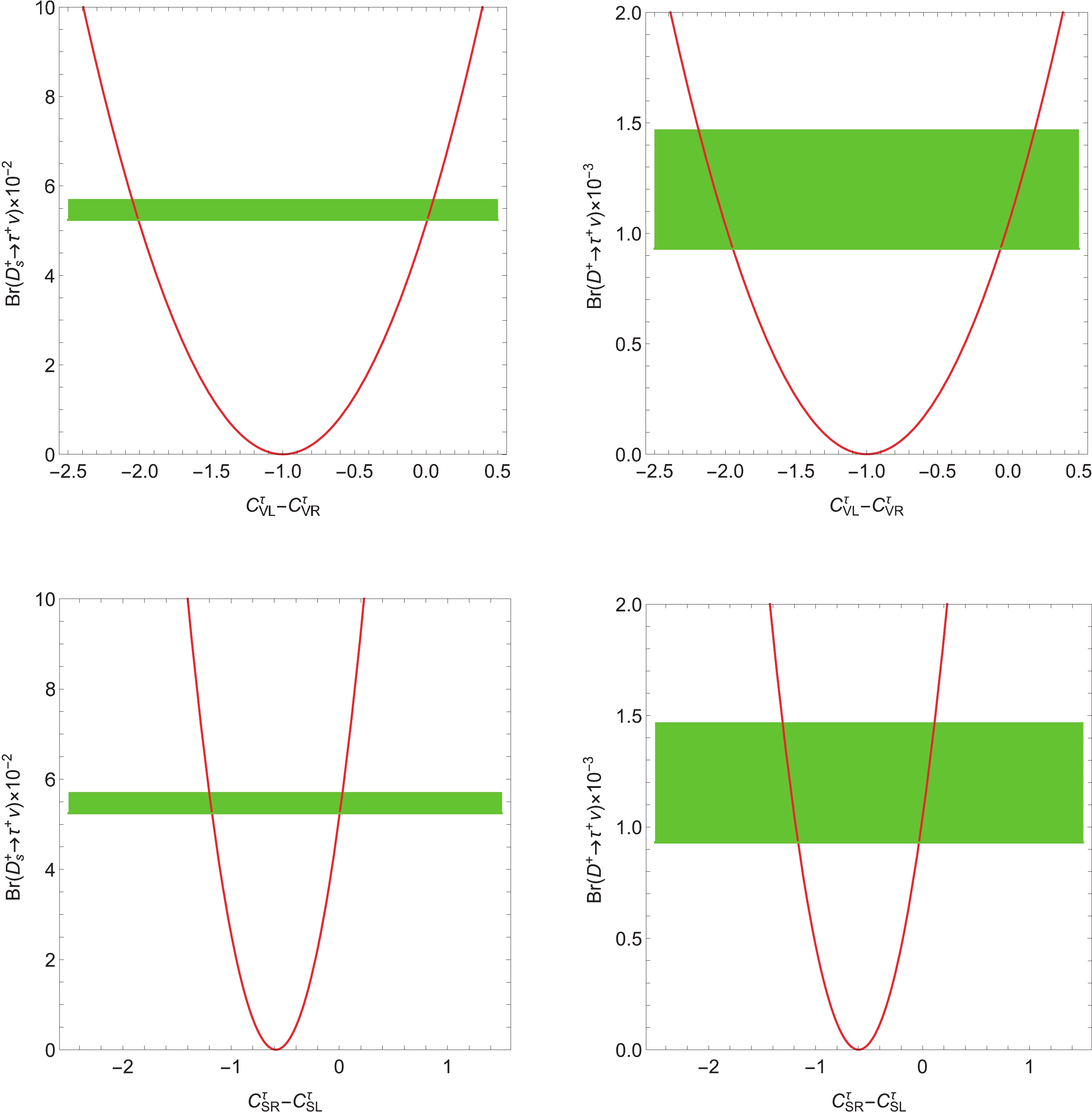
Figure 2. (color online) Dependence of
$\mathcal{B}(D^+ \to \tau^+ \nu_{\tau})$ and$\mathcal{B}(D_s^+ \to \tau^+ \nu_{\tau}) $ on$C_{VL}^\tau-C_{VR}^\tau$ and$C_{SR}^\tau-C_{SL}^\tau$ , respectively. The green bands represent the experimental data.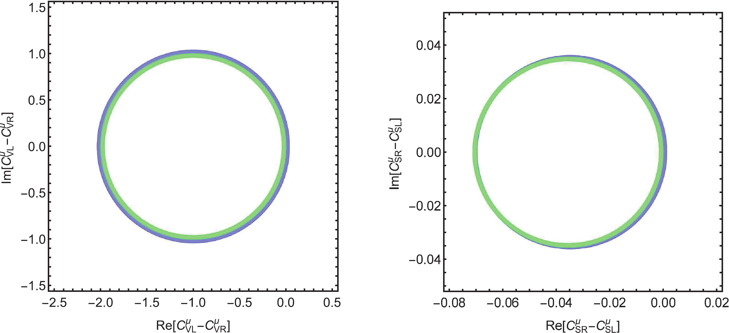
Figure 3. (color online) Allowed regions of the effective couplings
$C_{VL}^\mu-C_{VR}^\mu$ (left panel) and$C_{SR}^\mu-C_{SL}^\mu$ (right panel) extracted from the branching fractions of the decay modes$\mathcal{B}(D^+ \to \mu^+ \nu_{\mu})$ (green) and$\mathcal{B}(D_s^+ \to \mu^+ \nu_{\mu}) $ (blue), respectively.To test the lepton flavor universality, the ratio of two leptonic decays can be defined as [48]:
$ {\cal R}_{\ell_2}^{\ell_1} = \frac{{\cal{B}}(D_{(s)}^+ \rightarrow \ell_1^+ \nu_{\ell_1})}{{\cal{B}}(D_{(s)}^+ \rightarrow \ell_2^+ \nu_{\ell_2})}. $

(47) This observable is theoretically clean, as both uncertainties from the decay constants and the CKM matrix elements have been cancelled out by each other. Within the available experimental data, the constraints on each coefficient have been comprehensively discussed in Ref. [48]. Taking the
$ ({\cal R}^{\tau}_{\mu})^D $ as an example, we present the allowed parameter regions in Fig. 4. It can be determined that the SM predictions agree well with the current data and the allowed regions for NP are relatively limited.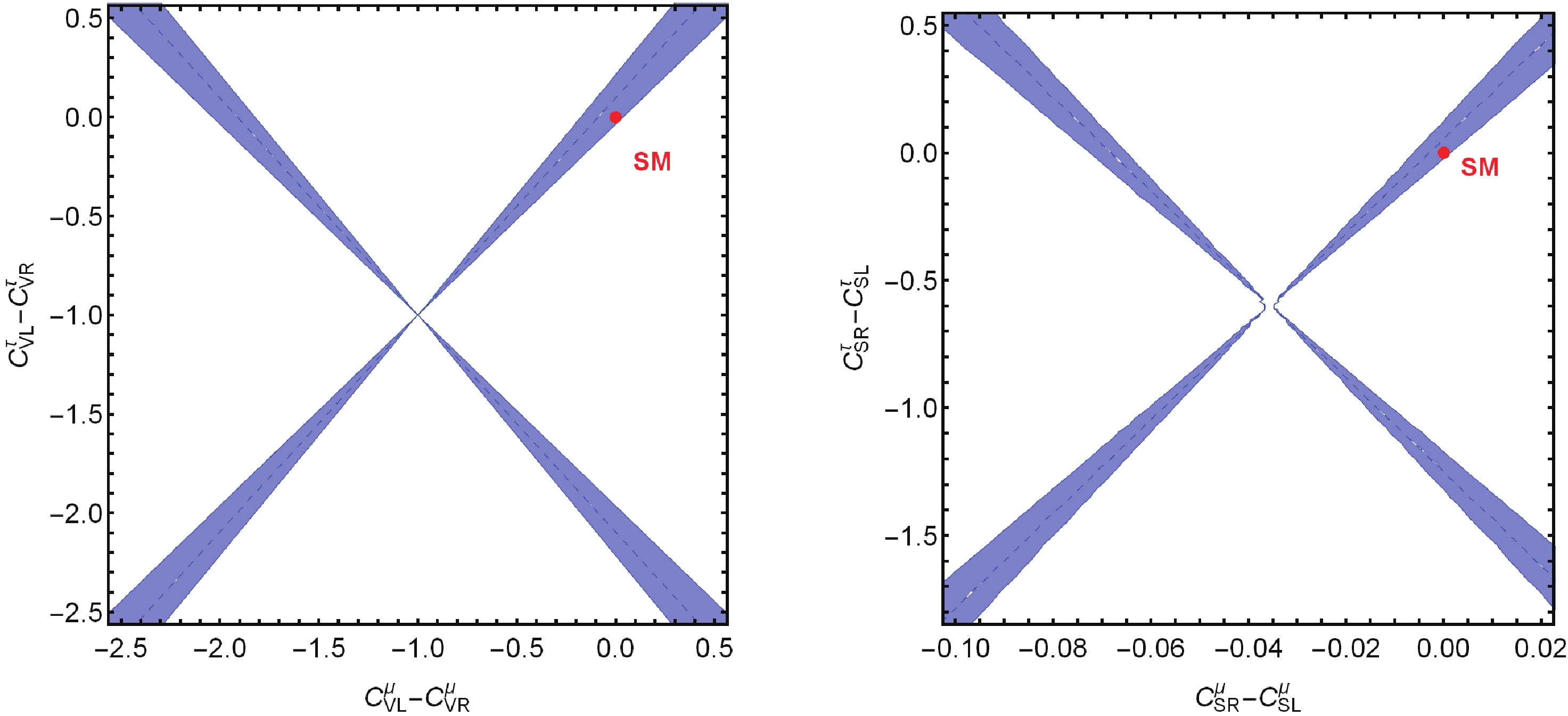
Figure 4. (color online) The allowed regions in the (
$C_{VL}^\mu-C_{VR}^\mu$ )-($C_{VL}^\tau-C_{VR}^\tau$ ) (left) and ($C_{SL}^\mu-C_{SR}^\mu$ )-($C_{SL}^\tau-C_{SR}^\tau$ ) (right) planes based on the ratio$({\cal R}^{\tau}_{\mu})^D$ , respectively. The red dots indicate the SM predictions. -
Due to the large mass of the
$ \tau $ lepton, the semileptonic D decays involving$ \tau $ lepton are kinematically forbidden. All decays can be divided into four categories according to the different currents:$ c\to s e^+\nu_e $ ,$ c\to s \mu^+\nu_\mu $ ,$ c\to d e^+\nu_e $ , and$ c\to d \mu^+\nu_\mu $ . In Table 6, we present the branching fractions of all semileptonic D decays in SM, where the only uncertainties arise from the form factors. The current experimental results [26] are also provided for comparison.Current Mode SM Experiment $ c\to s e^+\nu_e $ 

$ D^0\to K^-e^+\nu_e $ 

$ (3.49\pm0.23)\times 10^{-2} $ 

$ (3.542\pm 0.0035)\times 10^{-2} $ 

$ D^+\to \overline{K}^0e^+\nu_e $ 

$ (8.92\pm0.59)\times 10^{-2} $ 

$ (8.73\pm0.10)\times 10^{-2} $ 

$ D^0\to K^{*-}e^+\nu_e $ 

$ (1.92\pm0.17)\times 10^{-2} $ 

$ (2.15\pm0.16)\times 10^{-2} $ 

$ D^+\to \overline{K}^{*0}e^+\nu_e $ 

$ (4.98\pm0.45)\times 10^{-2} $ 

$ (5.40\pm0.10)\times 10^{-2} $ 

$ D_s^+\to \phi e^+\nu_e $ 

$ (2.46\pm0.42)\times 10^{-2} $ 

$ (2.39\pm0.16)\times 10^{-2} $ 

$ D_s^+\to \eta e^+\nu_e $ 

$ (1.55\pm0.33)\times 10^{-2} $ 

$ (2.29\pm0.19)\times 10^{-2} $ 

$ D_s^+\to \eta^\prime e^+\nu_e $ 

$ (5.91\pm1.26)\times 10^{-3} $ 

$ (7.4\pm1.4)\times 10^{-3} $ 

$ c\to s \mu^+\nu_\mu $ 

$ D^0\to K^-\mu^+\nu_\mu $ 

$ (3.40\pm0.22)\times 10^{-2} $ 

$ (3.41\pm 0.04)\times 10^{-2} $ 

$ D^+\to \overline{K}^0\mu^+\nu_\mu $ 

$ (8.69\pm0.57)\times 10^{-2} $ 

$ (8.76\pm0.19)\times 10^{-2} $ 

$ D^0\to K^{*-}\mu^+\nu_\mu $ 

$ (1.81\pm0.16)\times 10^{-2} $ 

$ (1.89\pm0.24)\times 10^{-2} $ 

$ D^+\to \overline{K}^{*0}\mu^+\nu_\mu $ 

$ (4.71\pm0.42)\times 10^{-2} $ 

$ (5.27\pm0.15)\times 10^{-2} $ 

$ D_s^+\to \phi\mu^+\nu_\mu $ 

$ (2.33\pm0.40)\times 10^{-2} $ 

$ (1.90\pm0.50)\times 10^{-2} $ 

$ D_s^+\to \eta\mu^+\nu_\mu $ 

$ (1.52\pm0.31)\times 10^{-2} $ 

$ (2.4\pm0.5)\times 10^{-2} $ 

$ D_s^+\to \eta^\prime \mu^+\nu_\mu $ 

$ (5.64\pm1.10)\times 10^{-3} $ 

$ (11.0\pm5.0)\times 10^{-3} $ 

$ c\to d e^+\nu_e $ 

$ D^0\to \pi^-e^+\nu_e $ 

$ (2.63\pm0.32)\times 10^{-3} $ 

$ (2.91\pm 0.04)\times 10^{-3} $ 

$ D^+\to \pi^0e^+\nu_e $ 

$ (3.41\pm0.41)\times 10^{-3} $ 

$ (3.72\pm0.17)\times 10^{-3} $ 

$ D^0\to \rho^-e^+\nu_e $ 

$ (1.74\pm0.25)\times 10^{-3} $ 

$ (1.77\pm0.16)\times 10^{-3} $ 

$ D^+\to \rho^0 e^+\nu_e $ 

$ (2.25\pm0.32)\times 10^{-3} $ 

$ (2.18^{+0.17}_{-0.25})\times 10^{-3} $ 

$ D^+\to \omega^0e^+\nu_e $ 

$ (1.91\pm0.27)\times 10^{-3} $ 

$ (1.69\pm0.11)\times 10^{-3} $ 

$ D^+\to \eta e^+\nu_e $ 

$ (0.76\pm0.16)\times 10^{-3} $ 

$ (1.11\pm0.07)\times 10^{-3} $ 

$ D^+\to \eta^\prime e^+\nu_e $ 

$ (1.12\pm0.24)\times 10^{-4} $ 

$ (2.0\pm0.4)\times 10^{-4} $ 

$ D_s^+\to K^0 e^+\nu_e $ 

$ (3.93\pm0.82)\times 10^{-3} $ 

$ (3.9\pm0.9)\times 10^{-3} $ 

$ D_s^+\to K^{*0} e^+\nu_e $ 

$ (2.33\pm0.34)\times 10^{-3} $ 

$ (1.8\pm0.4)\times 10^{-3} $ 

$ c\to d \mu^+\nu_\mu $ 

$ D^0\to \pi^-\mu^+\nu_\mu $ 

$ (2.60\pm0.31)\times 10^{-3} $ 

$ (2.67\pm 0.12)\times 10^{-3} $ 

$ D^+\to \pi^0\mu^+\nu_\mu $ 

$ (3.37\pm0.40)\times 10^{-3} $ 

$ (3.50\pm0.15)\times 10^{-3} $ 

$ D^0\to \rho^-\mu^+\nu_\mu $ 

$ (1.65\pm0.23)\times 10^{-3} $ 

$ -- $ 

$ D^+\to \rho^0 \mu^+\nu_\mu $ 

$ (2.14\pm0.30)\times 10^{-3} $ 

$ (2.4\pm0.4)\times 10^{-3} $ 

$ D^+\to \omega^0 \mu^+\nu_\mu $ 

$ (1.82\pm0.26)\times 10^{-3} $ 

$ -- $ 

$ D^+\to \eta\mu^+\nu_\mu $ 

$ (0.75\pm0.15)\times 10^{-3} $ 

$ -- $ 

$ D^+\to \eta^\prime\mu^+\nu_\mu $ 

$ (1.06\pm0.20)\times 10^{-4} $ 

$ -- $ 

$ D_s^+\to K^0\mu^+\nu_\mu $ 

$ (3.85\pm0.76)\times 10^{-3} $ 

$ -- $ 

$ D_s^+\to K^{*0}\mu^+\nu_\mu $ 

$ (2.23\pm0.32)\times 10^{-3} $ 

$ -- $ 

From this table, it can be observed that all theoretical predictions agree with the current experimental results at the
$ 1\sigma $ confidence level. Considering this table closely, we observe that for the$ D\to P \ell^+\nu_\ell $ , the differences between the theoretical predictions and the experimental data are very small, except the channels with$ \eta $ and$ \eta^\prime $ . As mentioned above,$ \eta $ and$ \eta^\prime $ are mixing states of$ \eta_1 $ ,$ \eta_8 $ , and a possible gluonic content. The mixing angles have not been determined yet, which creates significant theoretical uncertainties. Although some studies [56,57] indicated that the effects of mixing$ \rho^0-\phi-\omega $ may be important, for simplicity, we will not discuss these contributions. The branching fraction of the decay,$ D_s^+\to K^0 \mu^+\nu_\mu $ , has not been measured till now, and the order of magnitude is close to the corner in the BESIII experiment. For the$ D \to V \ell^+\nu_\ell $ decays, the predicted branching fractions of$ D^0\to K^{*-} e^+\nu_e $ ,$ D^0\to K^{*-} \mu^+\nu_\mu $ ,$ D^0\to \rho^{-} e^+\nu_e,$ and$ D^+\to \rho^{0} e^+\nu_e $ in SM agree well with experimental data, even for center values. However, for the decays,$ D^+\to \overline{K}^{*0}e^+\nu_e $ and$ D^+\to \overline{K}^{*0} \mu^+\nu_\mu $ , the SM results are slightly smaller than the data with more significant theoretical uncertainties. In contrast, the predicted branching fractions of$ D_s^+\to \phi \mu^+\nu_\mu $ and$ D_s^+\to \overline{K}^{*0}e^+\nu_e $ are larger than the experimental data, although there are larger uncertainties on both theoretical and experimental sides. We also note that for the form factors of$ D \to K^* $ transition, there are large differences between results calculated within different approaches, which triggers significant theoretical uncertainties. For example, for the decays$ D^+\to \overline{K}^{*0}e^+\nu_e $ and$ D^+\to \overline{K}^{*0} \mu^+\nu_\mu $ , the branching fractions based on LQCD [46] are larger than those based on LCSR [32] by 25%. Because many form factors of$ D \to V $ of LQCD are presently absent, we adopt the results of LCSR to maintain consistency. Based on this, the reliable calculations of$ D \to V $ are needed, especially from LQCD, to match the more precise experimental data. -
As already mentioned, all decays are induced by
$ c\to s e^+\nu_e $ ,$ c\to s \mu^+\nu_\mu $ ,$ c\to d e^+\nu_e,$ and$ c\to d \mu^+\nu_\mu $ currents. To study the contributions of new physics, we discuss two cases. For Case-I, we maintain the LFU and assume that the Wilson coefficients of new physics operators are the same for the muon and electron. However, for Case-II, we assume that NP violates LFU and contributes differently to the electron and muon sectors. Differences between$ c\to d \ell^+\nu_\ell $ and$ c\to s \ell^+\nu_\ell $ were not further discussed.Considering all existing data, including those of leptonic and semileptonic decays, we can constrain the Wilson coefficients of each new physics operator under a single operator scenario. In the calculation, we perform the least
$ \chi^2 $ fit of the Wilson coefficients at the$ 1\sigma $ C.L. of the experiment and theory. In our methodology of the least$ \chi^2 $ fit, the$ \chi^2,$ as a function of the Wilson coefficient$ C_{X}^\ell,$ is defined as [58]$ \chi^2(C_{X}) = \sum\limits_{m = 1}^{\rm data}\frac{[O^{\rm th}_{m}(C_{X}^\ell)-O^{\rm exp}_{m}]^{2}}{\sigma^{2}_{O^{\rm th}_{m}}+\sigma^{2}_{O^{\rm exp}_{m}}}, $

(48) where
$O^{\rm th}_{m}(C_{X}^\ell)$ represents the theoretical predictions for different branching fractions, and$O^{\rm exp}_{m}$ represents the corresponding experimental measurements, which are all presented in Tables 5 and 6.$\sigma_{O^{\rm th}_{m}}$ and$\sigma_{O^{\rm exp}_{m}}$ represent the theoretical and experimental errors, respectively. In addition, because of the significant theoretical uncertainties in the form factors of$ D\to \eta^{(\prime)} $ , we will not adopt the$ D\to \eta^{(\prime)}\ell \nu_\ell $ data in the fitting.In Table 7, we present the fitted Wilson coefficients for two different cases with a single operator. For the operators
$ O_{VL} $ and$ O_{VR} $ , the related Wilson coefficients$ C_{VL} $ and$ C_{VR} $ , respectively, are in the order of$ {\cal O}(10^{-3}) $ in both cases. The results of Case-II indicate the violation of LFU for the operator$ O_{VL} $ ; however, such small effects are buried in the theoretical and experimental uncertainties. For the operators$ O_{SL} $ and$ O_{SR} $ in Case-I, their Wilson coefficients are also in the order of$ {\cal O}(10^{-3}) $ , and the effects of this phenomenon cannot be determined in the current experiments. In fact, the most stringent constraints originate from the pure leptonic decays. Therefore, in Case-II,$ C_{SL}^\mu $ and$ C_{SR}^\mu $ are in the order of$ {\cal O}(10^{-2}) $ and have relatively small uncertainties. However, for the decays$ D\to e^+\nu_e $ , only the upper limits are available, the fitted$ C_{SL}^e $ and$ C_{SR}^e $ are in the order of$ {\cal O}(10^{-4}) $ , with very significant uncertainties. Regarding the Wilson coefficients of the tensor operators that are only constrained by the semi-leptonic D decays,$ C_{T}^\ell $ can be in the order of$ {\cal O}(10^{-2}) $ . From these results, all new Wilson coefficients are less than 8%, which poses stringent constraints on new physics models,$ W^\prime $ models [6,7], leptoquark models [9-11], and models with charged Higgs [13-15]. Moreover, we note that LFU might be violated by the operators,$ O_{SL}^\ell $ and$ O_{SR}^\ell $ , which can be investigated further in other observables. We acknowledge that our analyses depend on the$ D\to V $ form factors, and that more precise form factors in future will help us to improve our results.Case Wilson Coefficient Fitted Results $ \chi^{2}_{1\sigma}/{\rm d.o.f} $ 

Case-I $ C_{VL}^\ell $ 

$ (4.3\pm 9.6)\times 10^{-3} $ 

$ 10.1/21 $ 

$ C_{VR}^\ell $ 

$ (2.7\pm 9.8)\times 10^{-3} $ 

$ 10.2/21 $ 

$ C_{SL}^\ell $ 

$ (0.3\pm 0.6)\times 10^{-3} $ 

$ 10.0/21 $ 

$ C_{SR}^\ell $ 

$ (-0.3\pm 0.6)\times 10^{-3} $ 

$ 10.0/21 $ 

$ C_{T}^\ell $ 

$ (-31.0\pm 30.0)\times 10^{-3} $ 

$ 6.3/19 $ 

Case-II $ C_{VL}^e $ 

$ (9.9\pm 16.2)\times 10^{-3} $ 

$ 4.4/11 $ 

$ C_{VR}^e $ 

$ (2.6\pm 16.9)\times 10^{-3} $ 

$ 4.8/11 $ 

$ C_{SL}^e $ 

$ (0.4\pm 0.6)\times 10^{-3} $ 

$ 4.8/11 $ 

$ C_{SR}^e $ 

$ (-0.4\pm 0.6)\times 10^{-3} $ 

$ 4.8/11 $ 

$ C_{T}^e $ 

$ (-43\pm 42)\times 10^{-3} $ 

$ 4.5/11 $ 

$ C_{VL}^\mu $ 

$ (1.4\pm 11.9)\times 10^{-3} $ 

$ 5.5/9 $ 

$ C_{VR}^\mu $ 

$ (2.7\pm 12.0)\times 10^{-3} $ 

$ 5.4/9 $ 

$ C_{SL}^\mu $ 

$ (70.2\pm 90.0)\times 10^{-3} $ 

$ 3.1/9 $ 

$ C_{SR}^\mu $ 

$ (-70.2\pm 90.0)\times 10^{-3} $ 

$ 3.1/9 $ 

$ C_{T}^\mu $ 

$ (-28.2\pm 25.3)\times 10^{-3} $ 

$ 1.7/7 $ 

Table 7. Fitted values of the Wilson coefficients for different cases.
-
First, we study the pure leptonic D decays with the electron final state. As expressed in Eq. (46), the branching fractions are very sensitive to the
$ O^e_{SL} $ and$ O^e_{SR} $ operators because their contributions are related to$ 1/m_e $ . With the contributions from interactions with the$ O^e_{SL} $ or$ O^e_{SR} $ operator, the branching fractions of these pure leptonic D decays are predicted to be$ {\cal{B}}(D^+ \rightarrow e^+ \nu_{e}) = (1.6^{+19.6}_{-0.7})\times 10^{-8}; $

(49) $ \begin{array}{l} {\cal{B}}(D_s^+ \rightarrow e^+ \nu_{e}) = (2.4^{+27.6}_{-1.2})\times 10^{-7}, \end{array} $

(50) where the uncertainties solely originate from the fitted Wilson coefficients. Compared to the SM results in Table 5, the current branching fractions are approximately twice as large as the SM predictions with relatively significant uncertainties. According to Eq. (47), the ratios can be calculated as
$ ({\cal R}_{\mu}^e)^{D^+} = \frac{{\cal{B}}(D^+ \rightarrow e^+ \nu_{e})}{{\cal{B}}(D^+ \rightarrow \mu^+ \nu_{\mu})_{\rm Ex}} = (4.3^{+52.4}_{-2.0})\times 10^{-5}, $

(51) $ ({\cal R}_{\mu}^e)^{D_s^+} = \frac{{\cal{B}}(D_{s}^+ \rightarrow e^+ \nu_{e})}{{\cal{B}}(D_{s}^+ \rightarrow \mu^+ \nu_{\mu})_{\rm Ex}} = (4.4^{+50.7}_{-2.1})\times 10^{-5}; $

(52) which are larger than the SM predictions:
$ \begin{array}{l} ({\cal R}_{\mu}^e)^{D^+}\simeq ({\cal R}_{\mu}^e)^{D_s^+} = 2.3\times 10^{-5}. \end{array} $

(53) However, the orders of these magnitudes are too small to be measured now. We hope that future high intensity experiments can evaluate the above results.
Secondly, we study the effects of NP in semileptonic D decays. From Table 7, it is observed that for the decays with electron final state, the Wilson coefficients,
$ C_{VL,VR}^e $ and$ C_{SL,SR}^e $ , are too small in both cases to affect the branching fractions and other observables, such as the differential widths, forward-backward asymmetries, longitudinal polarizations of the final state vector mesons, and helicity asymmetries of electrons. Regarding$ C_T^e $ , its influence is substantially similar to the decays with the muon final state that will be discussed later. On the experimental perspective, all the absolute branching fractions have been measured, and the results obtained agree well with the SM predictions with uncertainties, as presented in Table 6. However, the$ q^2 $ -dependencies of the differential branching fractions, forward-backward asymmetries, and longitudinal polarizations of final vector mesons have not yet been completely measured to date. In Fig. 5, we consider the decays$ D^0 \to K^-e^+\nu_e $ ,$ D^0 \to K^{*-}e^+\nu_e $ ,$ D_s^+ \to \phi e^+\nu_e $ ,$ D^0 \to $ $ \pi^-e^+\nu_e $ ,$ D^0 \to \rho^-e^+\nu_e $ ,$ D_s^+ \to K^0e^+\nu_e $ and$ D_s^+ \to K^{*0}e^+\nu_e $ as examples, and plot the$ q^2 $ -dependencies of the above mentioned observables. Because the mass of the electron is negligible, the electron helicity asymmetries are approximately$ -1 $ , such that any significant deviation from -1 would be a signal of NP. We expect these predictions to be well tested in BESIII, Belle II, and other future high luminosity experiments.
Figure 5. (color online) The
$q^2$ -dependence of the branching fractions${\rm d}B/{\rm d} q^2$ , forward-backward asymmetries of the leptonic side$A_{FB}(q^2)$ , and longitudinal polarization components of the vector mesons in SM.Finally, we investigate the NP effects in the semileptonic D decays with muon final state. Again, it is observed from Table 7 that the Wilson coefficients
$ C^\mu_{SL(R)} $ and$ C_T^\mu $ are in the order of$ 10^{-2} $ . Although such Wilson coefficients are not sufficient to significantly alter the branching fractions, they may affect other observables. To verify their effects, we consider the decays$ D^0 \to K^-\mu^+\nu_\mu $ ,$ D^0 \to K^{*-}\mu^+\nu_\mu $ ,$ D_s^+ \to \phi \mu^+\nu_\mu $ ,$ D^0 \to $ $ \pi^-\mu^+\nu_\mu $ ,$ D^0 \to \rho^- \mu^+ \nu_\mu $ ,$ D_s^+ \to K^0\mu^+\nu_\mu $ and$ D_s^+ \to K^{*0}\mu^+\nu_\mu $ as examples, and investigate their contributions to the$ q^2 $ -dependencies of the differential widths, forward-backward asymmetries, longitudinal polarizations of final vector mesons, and helicity asymmetries of the muon; the obtained results are presented in Figs. 6, 7, 8, and 9, respectively. From these figures, it can be observed that for the decays$ D \to V \ell^+\nu_\ell $ , the Wilson coefficient of the tensor operator affects these observables without altering their shapes, and the Wilson coefficients of other operators barely affect these observables. Therefore, if significant deviations were measured in the future, interactions with tensor operator would be preferable.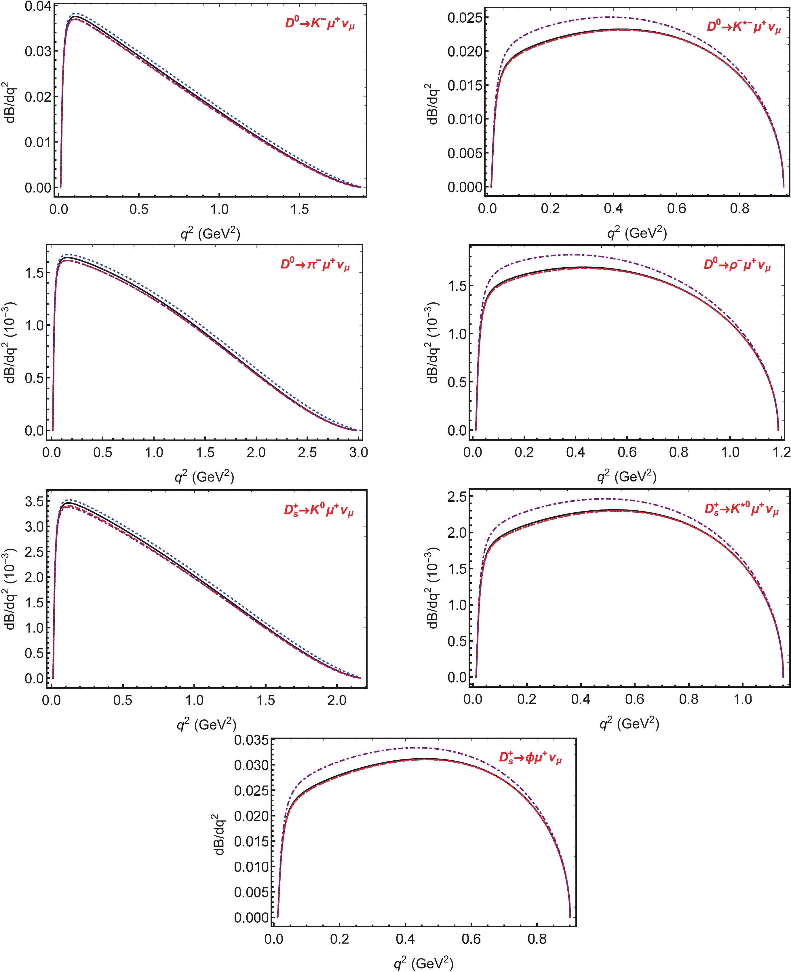
Figure 6. (color online) The
$q^2$ -dependence of the differential branching fractions${\rm d} B/{\rm d} q^2$ of$D^0 \to K^-\mu^+\nu_\mu$ ,$D^0 \to K^{*-}\mu^+\nu_\mu$ ,$D^0 \to \pi^-\mu^+\nu_\mu$ ,$D^0 \to \rho^-\mu^+\nu_\mu$ ,$D_s^+ \to K^0\mu^+\nu_\mu$ ,$D_s^+ \to K^{*0}\mu^+\nu_\mu$ and$D_s^+ \to \phi \mu^+\nu_\mu$ with fitted values for decays. The solid (black) lines depict the predictions of SM, whereas the dotted (blue), dashed (red), and dot-dashed (purple) lines denote NP predictions corresponding to the best-fit Wilson coefficients of${\cal O}_{SL}$ ,${\cal O}_{SR}$ , and${\cal O}_{T}$ , respectively.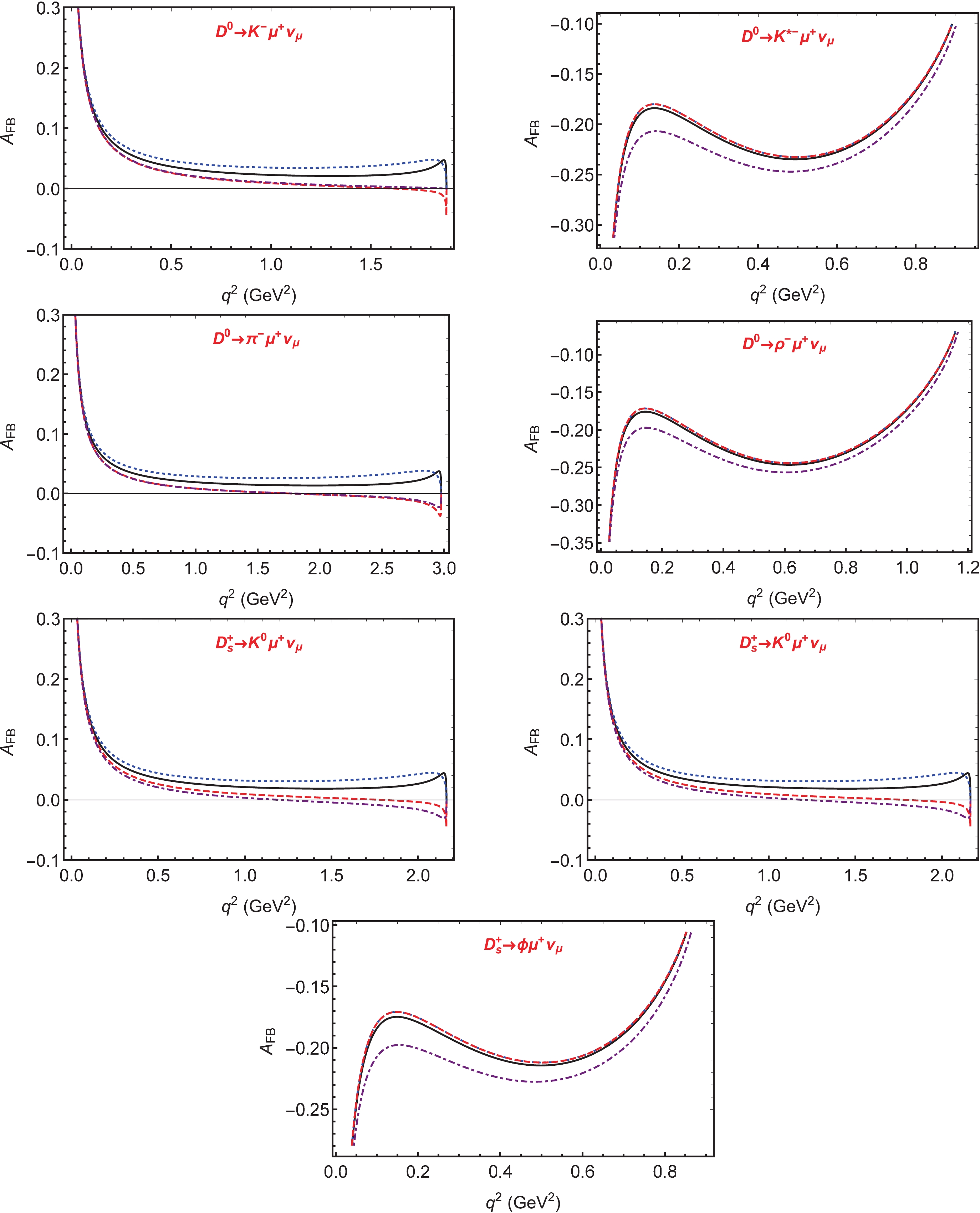
Figure 7. (color online) Predicted
$q^2$ -dependence of the forward-backward asymmetries of$D^0 \to K^-\mu^+\nu_\mu$ ,$D^0 \to K^{*-}\mu^+\nu_\mu$ ,$D^0 \to \pi^-\mu^+\nu_\mu$ ,$D^0 \to \rho^-\mu^+\nu_\mu$ ,$D_s^+ \to K^0\mu^+\nu_\mu$ ,$D_s^+ \to K^{*0}\mu^+\nu_\mu$ and$D_s^+ \to \phi \mu^+\nu_\mu$ with fitted values for decays. The solid (black) lines depict the predictions of SM, whereas the dotted (blue), dashed (red), and dot-dashed (purple) lines denote NP predictions corresponding to the best-fit Wilson coefficients of${\cal O}_{SL}$ ,${\cal O}_{SR}$ , and${\cal O}_{T}$ , respectively.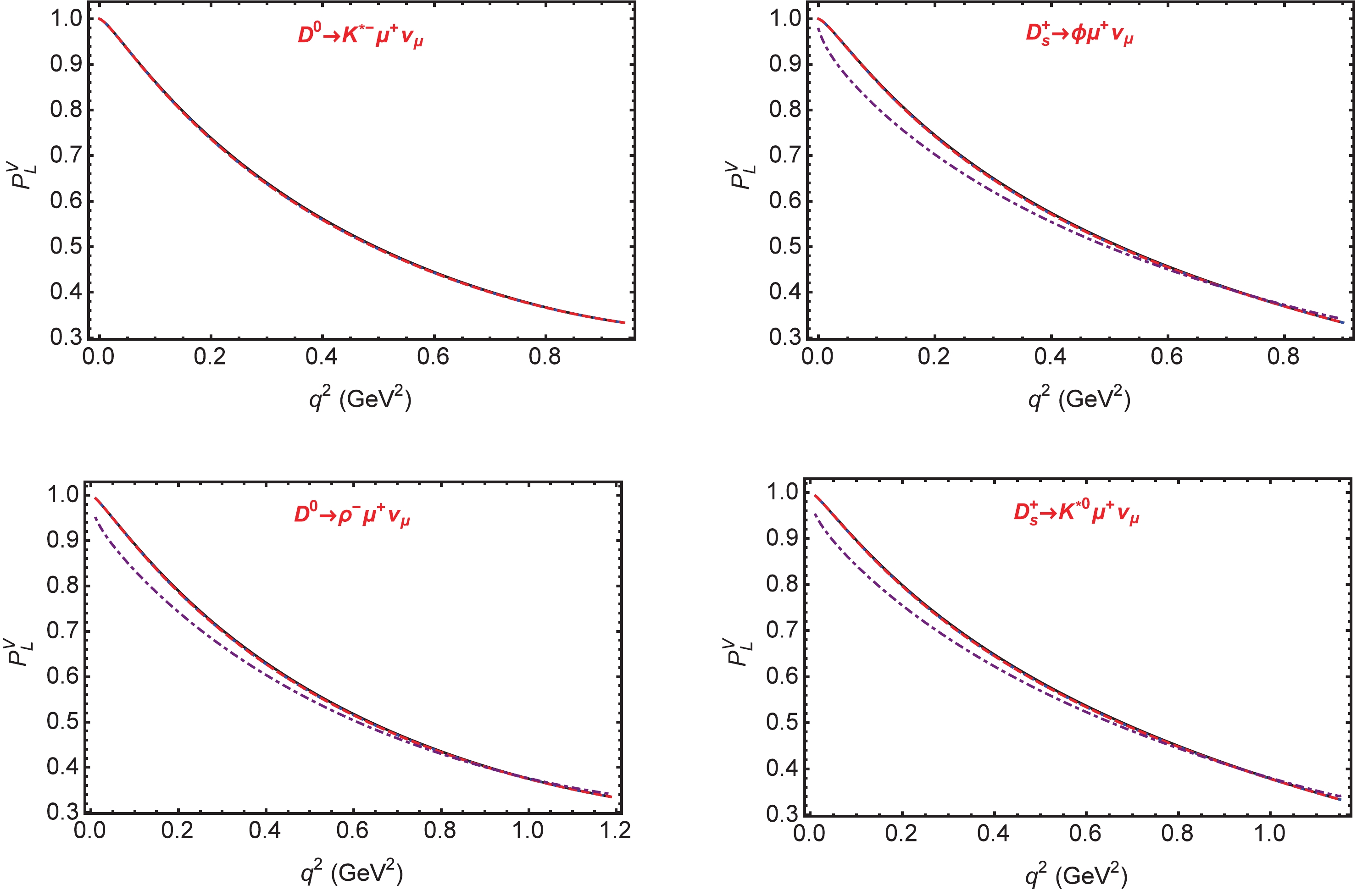
Figure 8. (color online) Predicted
$q^2$ -dependence of the longitudinal polarization of the final vector mesons of$D^0 \to K^{*-}\mu^+\nu_\mu$ ,$D_s^+ \to \phi \mu^+\nu_\mu$ ,$D^0 \to \rho^-\mu^+\nu_\mu$ and$D_s^+ \to K^{*0}\mu^+\nu_\mu$ with fitted values for decays. The solid (black) lines denote the predictions of SM, while the dotted (blue), dashed (red) and dotdashed (purple) lines represent NP predictions corresponding to the best-fit Wilson coefficients of${\cal O}_{SL}$ ,${\cal O}_{SR}$ , and${\cal O}_{T}$ , respectively.
Figure 9. (color online) Predicted
$q^2$ -dependence of the lepton helicity asymmetries of$D^0 \to K^-\mu^+\nu_\mu$ ,$D^0 \to K^{*-}\mu^+\nu_\mu$ ,$D^0 \to \pi^-\mu^+\nu_\mu$ ,$D^0 \to \rho^-\mu^+\nu_\mu$ ,$D_s^+ \to K^0\mu^+\nu_\mu$ ,$D_s^+ \to K^{*0}\mu^+\nu_\mu$ and$D_s^+ \to \phi \mu^+\nu_\mu$ with fitted values for decays. The solid (black) lines denote the predictions of SM, while the dotted (blue), dashed (red) and dotdashed (purple) lines represent NP predictions corresponding to the best-fit Wilson coefficients of${\cal O}_{SL}$ ,${\cal O}_{SR}$ , and${\cal O}_{T}$ , respectively.Regarding the
$ D \to P \ell^+\nu_\ell $ decays, the differential widths are also not sensitive to the fitted Wilson coefficients of NP operators. In contrast, the forward-backward asymmetries$ A_{FB}(q^2) $ and muon helicity asymmetries$ P_F^\ell(q^2) $ are very sensitive to the fitted Wilson coefficients, especially to those of the scalar and tensor operators, as illustrated in Figs. 7 and 9. We consider the decay$ D^0 \to K^-\mu^+\nu_\mu $ induced by$ c\to s \mu^+ \nu_\mu $ as an example for illustration. For the forward-backward asymmetry$ A_{FB}(q^2) $ , it is always positive in SM. In the decay distribution expressed in Eq. (32),$ A_3^P $ is dominant in the low$ q^2 $ region. Because$ A_3^P $ is not related to the NP operators, their contributions are not significant. However, in the large$ q^2 $ region,$ A_1^P $ becomes significant. Because$ A_1^P $ depends on$ |C_{SL}+C_{SR}|^2 $ and$ |C_T|^2 $ , the large deviation from the SM prediction in the large$ q^2 $ region is logical. Furthermore, it is determined that with the fitted$ C_{SR}^\mu $ , the forward-backward asymmetries of decays$ D^0 \to K^-\mu^+\nu_\mu $ ,$ D^0 \to \pi^-\mu^+\nu_\mu,$ and$ D_s^+ \to K^0\mu^+\nu_\mu $ cross the zero points, when$ q^2 = 1.57\; {\rm GeV}^2 $ ,$ 1.71\; {\rm GeV}^2,$ and$ 1.76\; {\rm GeV}^2 $ , respectively. This unique behavior can be used to probe the right-handed scalar current. Similarly, for the$ D^0 \to K^-\mu^+\nu_\mu $ ,$ D^0 \to \pi^-\mu^+\nu_\mu,$ and$ D_s^+ \to K^0\mu^+\nu_\mu $ decays, when$ q^2>0.5\; {\rm GeV}^2 $ , the contributions of scalar operators become significant and can influence the helicity asymmetries of the muon$ P_F^\mu $ , as illustrated in Fig. 9. In addition, both$ A_{FB} $ and$ P_F^\ell $ of$ D\to P\ell\nu $ decays are proportional to the dynamic factor$ \sqrt{Q_+Q_-} $ , which implies that these two asymmetries are equal to zero when$ q^2 = (m_D-m_P)^2 $ , as illustrated in Figs. 7 and 9. However, the proportion does not hold in the corresponding observables of$ D\to V\ell\nu $ decays. Consequently, this behavior disappears in the panels of$ D\to V\ell\nu $ decays. Because all the above observables have not been measured, we suggest that our experimental colleagues measure these parameters, to determine the possible contributions of NP. -
Recent
$ B \to D^{(*)}\ell^- \bar\nu_\ell $ anomalies imply that NP may appear in the charged current$ b\to c \ell^- \bar\nu_\ell $ ; hence, it is natural to raise questions about such phenomena in the D decays induced by$ c\to (s,d)\ell^+\nu_\ell $ transitions. However, current experimental measurements on the charm meson decay observables are consistent with the SM predictions. Such consistency enables us to constrain the parameter spaces of NP and to further test NP models. In this work, we extended the SM by assuming general effective Lagrangian describing the$ c\to (s,d)\ell^+\nu_\ell $ transitions, which consists of the full set of the four-fermion operators. With the latest experimental data, we performed the least$ \chi^2 $ fit of the Wilson coefficient corresponding to each operator in two different cases. We determined that the Wilson coefficients of scalar and tensor operators can be in the order of$ {\cal O}(10^{-2}) $ , whereas those of the vector operators are in the order of$ {\cal O}(10^{-3}) $ . With the fitted Wilson coefficients, we calculated the differential branching fractions, forward-backward asymmetries, longitudinal polarizations of the final state vector mesons, and lepton helicity asymmetries of leptons. The pure leptonic decays that are very sensitive to the interactions with scalar operators can be adopted to constrain the scalar Wilson coefficients and test models with charged Higgs. For the semileptonic decays with the electron final state, the effects of NP are negligible, and any deviation from SM predictions would create significant challenges for the SM and its extensions. Regarding the semileptonic decays with the muon final state, the interactions with scalar or tensor operators influence the forward-backward asymmetries and muon helicity asymmetries of$ D \to P\mu^+ \nu_\mu $ . Future measurements on the studied observables in the BESIII and Belle II experiments will help us investigate the effects of NP. -
We thank Dr. Ivan Nisandzic and Prof. Hai-Long Ma for their valuable discussions.
Investigation on effects of new physics in ${ { c}\to{{ (s,d)}}\ell^+\nu_\ell} $ transitions
- Received Date: 2021-02-21
- Available Online: 2021-06-15
Abstract: Anomalies in decays induced by


 DownLoad: