


 Abstract
 HTML
HTML Reference
 Related
 PDF
PDF


-
The nucleus-nucleus interaction potential, which includes the short-range attractive and absorptive nuclear potential and long-range repulsive Coulomb potential, has always been a major issue in nuclear physics. The Coulomb interaction between two nuclei is well known, but the nuclear component is much more difficult to describe. Over the last decades, the optical model potential (OMP) has been widely used to describe the nuclear component, and several different potential forms have been proposed to reproduce a large volume of nuclear reaction data [1-3]. In addition to the nuclear reactions induced by light particles, the nuclear reactions between heavy ions can also be described by the optical model [3-6].
Elastic scattering, the simplest nuclear reaction process, is often used to understand more complicated reaction channels [7]. The optical potential parameters extracted by fitting elastic scattering data can be used to obtain information from the nucleus. A large number of systematic optical parameters have been presented as reliable optical potential parameters for reactions of different systems and different incident energies [3]. In this way, one can acquire the optical potential parameters directly without fitting elastic scattering data. Most of these works focus on the reactions induced by light particles such as protons, neutrons, deuterons, and helium-4 [8-11]. Because of the strong Coulomb interaction between heavy-ions, systematic research on the optical potential between heavy ions is substantially more difficult and scarce than research on reactions induced by light particles. However, considerable progress has been made in recent years. Based on the double folding potential and Pauli nonlocality, Chamon et al. [12] proposed the well-known S
$ \tilde{a} $ o Paulo potential (SPP). The work provides a systematic description of the realistic nucleus-nucleus interaction, and it can be applied to various reaction systems including stable and unstable particles. A modified Woods-Saxon potential based on the Skyrme energy-density functional approach was proposed by Wang et al. [13, 14] to provide a global description of nucleus-nucleus interactions. Not only elastic scattering but also the fusion barrier and fission barrier of fusion-fission reactions can be described using this potential. By analyzing the angular distributions of$ ^{6,7}{\rm{Li}} $ elastic scattering from heavy-ions, Xu and Pang proposed a systematic single-folding potential. These systematics can provide a reasonable account of both the elastic scattering and total reaction cross sections [15]. We propose a systematic six-parameter Woods-Saxon potential with fixed imaginary parameters based on the elastic scattering angular distributions induced by 12C [16]. It is not satisfactory for some elastic scattering at energies around the Coulomb barriers or higher than 300 MeV, which may be attributable to the fixed imaginary potential parameters.In the present work, the Woods-Saxon shape is adopted for both the real and imaginary parts, and the imaginary parameters are also studied as variables. Experimental elastic scattering angular distributions of 11B, 12C, and 16O + heavy-ions are used to extract the optical potential parameters.
-
The Woods-Saxon model potential was proposed by Woods and Saxon to approximate the shape of the nuclear component of nucleus-nucleus interactions [17]. Although it is a phenomenological approximation, reactions of different incident energies and different projectile-target combinations can be well reproduced with the six parameters used in the calculations [7].
The six-parameter Woods-Saxon potential contains a real component and an imaginary component and is expressed as
$ V_n(r) = -\frac{V}{1+{\rm e}^{(r-R_V)/a_V}}-\frac{{\rm i}W}{1+{\rm e}^{(r-R_W)/a_W}}, $

(1) where V and W are potential depth parameters for the real and imaginary potentials, respectively;
$ R_i $ =$ r_i(A_1^{1/3}+ $ $ A_2^{1/3}) $ , in which$ i = V, \;W $ , denotes the real and imaginary radius parameters;$ a_V $ and$ a_W $ respectively refer to the real and imaginary diffuseness; and$ A_{1} $ and$ A_{2} $ are the mass numbers of the projectile and target nuclei.The Coulomb potential is always expressed as
$ V_{\rm C}(r) = \left\{ \begin{array}{l} \dfrac{Z_1Z_2e^2}{2R_{\rm C}}\left(3-\dfrac{r^2}{R_{\rm C}^2}\right) \quad r < R_{\rm C}, \\ \dfrac{Z_1Z_2e^2}{r} \quad r > R_{\rm C}, \\ \end{array}\right. $

(2) where
$ R_{\rm C} = r_{\rm C}(A_1^{1/3}+A_2^{1/3}) $ is the radius parameter. It has been proved that theoretical angular distributions are not sensitive to changes in the Coulomb radius [18]. Therefore, a fixed$ r_{\rm C} $ equal to 1.0 fm is used throughout the following processes.In the present work, 27 sets of elastic scattering angular distribution data are adopted to extract the Woods-Saxon potential parameters. The targets range from 12C to 209Bi, and the incident energies range from 25 to 420 MeV. Most of the data are from the National Nuclear Data Center, while the angular distributions of 12C elastic scattering from 90Zr, 91Zr, 96Zr , and 116Sn were measured at the China Institute of Atomic Energy (CIAE), Beijing. Because the optical potential parameters have large ambiguities, several different sets of parameter combinations can reproduce the experimental data well [19]. It has been confirmed that when fitting two or more optical potential parameters at the same time, we easily fall into a minimum trap. In order to study the intrinsic relationship between these parameters, we define more than 1 million sets of parameter combinations of W,
$ R_V $ ,$ R_W $ ,$ a_V $ , and$ a_W $ in advance and then use each of them to fit V for all the data. W varies in the range of 10 - 300 MeV by steps of 2 MeV. The geometric parameters of the real and imaginary components are set to the same value, i.e.,$ r_V $ =$ r_W $ , and vary between 0.5 and 1.5 fm in increments of 0.01 fm. Finally,$ a_V $ =$ a_W $ vary between 0.3 and 1.0 fm in increments of 0.01 fm. The analysis process can be divided into four steps:1) Use all the parameter combinations to fit each elastic scattering dataset with the nuclear reaction code PTOLEMY [20]. In this way, the output V and corresponding
$ \chi^2 $ are obtained for every calculation.2) Analyze the correlation of
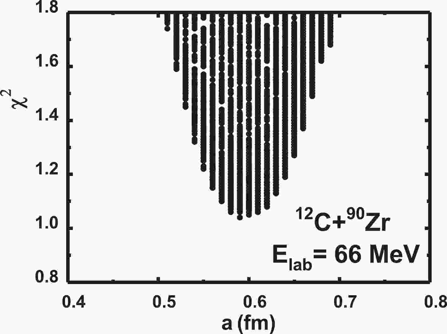
$ \chi^2 $ with the depth, radius, and diffuseness parameters. We find that, for each system, there exists a suitable value of the diffuseness parameter that gives the minimum$ \chi^2 $ . As a typical result, Figure 1 shows$ \chi^2 $ versus the diffuseness parameter for 12C + 90Zr elastic scattering. However, the depth and radius parameters cannot be extracted in the same way as the diffuseness parameter because there are no best fit values for these parameters. We list the extracted diffuseness for each interaction system in Table 1. The analysis of the diffuseness uncertainties employs the$ \chi^2 $ envelope method proposed in Ref. [21]. A linear formula for the diffuseness parameter a versus$ A_1^{1/3}+A_2^{1/3} $ is summarized in Eq. (3) and shown in Fig. 2; the uncertainties of the slope and intercept are 0.011 and 0.063 fm, respectively. The slope is negative, indicating that as the mass of the system increases, the diffuseness parameter tends to decrease.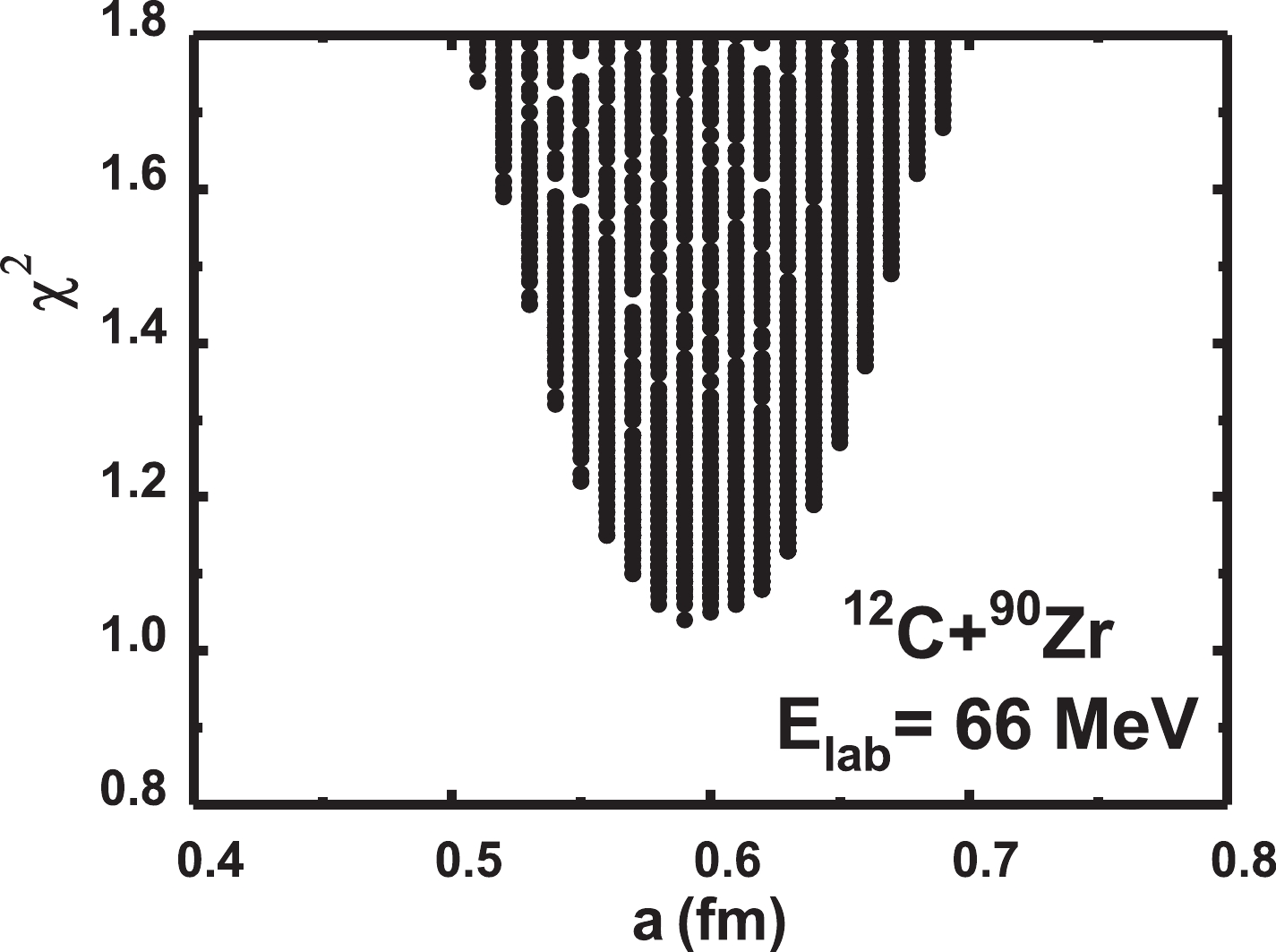
Figure 1.
$\chi^2$ versus the diffuseness parameter for 12C + 90Zr at 66 MeV. Each dot represents a parameter set. It is found that a = 0.59 fm corresponds to the minimum$\chi^2$ .Reaction $E_{\rm lab}$ /MeV

a/fm $\Delta a$ /fm

11B+58Ni 25 0.64 0.03 11B+58Ni 35 0.54 0.03 12C+12C 158 0.72 0.02 12C+12C 360 0.75 0.03 12C+13C 127.2 0.74 0.03 12C+16O 76.8 0.61 0.02 12C+19F 40.3 0.67 0.02 12C+19F 50 0.76 0.02 12C+19F 60 0.73 0.02 12C+40Ca 180 0.69 0.03 12C+40Ca 300 0.69 0.04 12C+40Ca 420 0.74 0.03 12C+64Ni 48 0.59 0.06 12C+90Zr 66 0.59 0.03 12C+90Zr 120 0.71 0.04 12C+90Zr 180 0.68 0.04 12C+90Zr 300 0.66 0.07 12C+90Zr 420 0.71 0.06 12C+91Zr 66 0.64 0.03 12C+96Zr 66 0.58 0.08 12C+116Sn 66 0.51 0.06 12C+169Tm 84 0.44 0.04 12C+208Pb 58.9 0.40 0.07 12C+209Bi 87.4 0.54 0.04 16O+64Zn 48 0.66 0.07 16O+68Zn 52 0.56 0.08 16O+209Bi 90 0.46 0.05 Table 1. The most suitable diffuseness parameters extracted in the analysis.
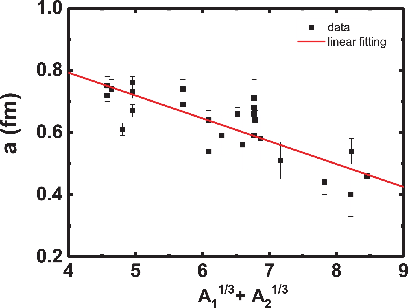
Figure 2. (color online) The diffusion parameter as a function of
$A_1^{1/3}+A_2^{1/3}$ .$ a_V = a_W = -0.0736(A_1^{1/3}+A_2^{1/3})+1.087\ \ {\rm{(fm)}}. $

(3) 3) When the diffuseness parameters are fixed as in Eq. (3), we find a correlation between the depth and radius parameters with the real and imaginary parts, respectively. As an example,
$ \chi^2 $ versus the depth parameters of 12C + 90Zr elastic scattering at 66 MeV is shown in Fig. 3. It is obvious that the curve for V is much steeper than that for W, which indicates that$ \chi^2 $ is more sensitive to V than to W. Each curve corresponds to a specific radius parameter value, and the correlations of the depth and radius parameter combinations of best fit are as follows: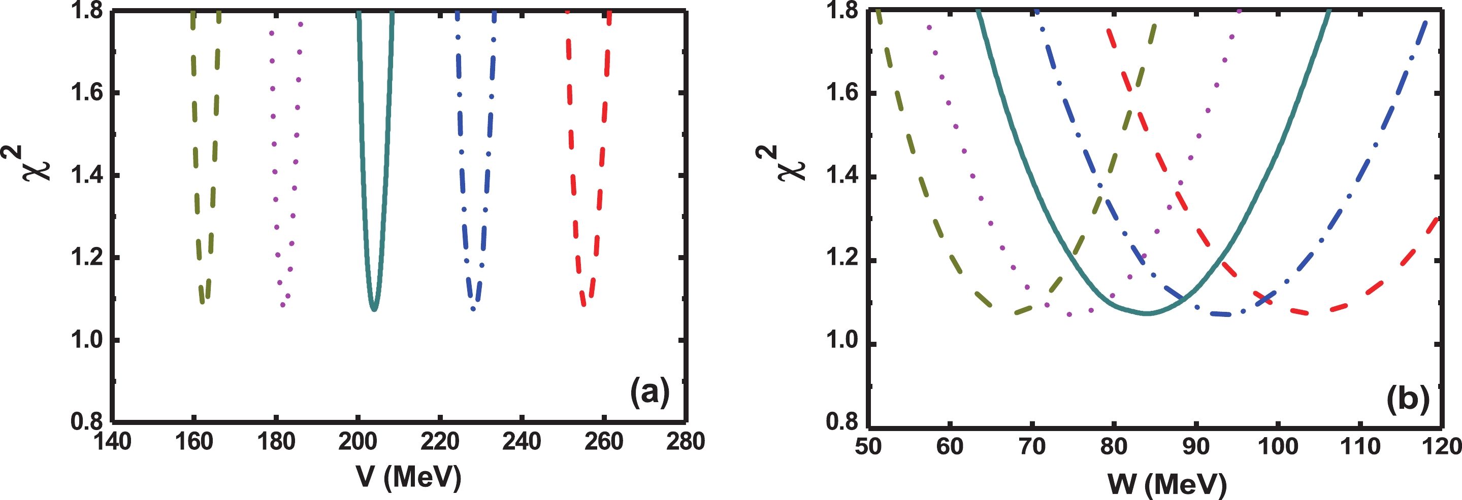
Figure 3. (color online)
$\chi^2$ versus V (a) and W (b) for 12C + 90Zr at 66 MeV. Each curve corresponds to a different radius parameter; the valleys give almost the same$\chi^2$ . The radius parameters for each curve from left to right are 1.07 to 1.03 fm, by steps of 0.01 fm. Observe that the curves for V (a) are much steeper than those for W (b).$ \begin{split} &V\times {\rm exp}(R_V/a_V) = const1,\\ &W\times {\rm exp}(R_W/a_W) = const2. \end{split} $

(4) The values of
$ const1 $ and$ const2 $ are listed in Table 2. The errors stem from the uncertainties of the diffuseness parameters. Since the radius parameter and diffuseness parameter are the same for the real and imaginary components, the ratio of W to V is equal to the ratio of$ const2 $ to$ const1 $ .Reaction $E_{\rm lab}{\rm{ /MeV}}$ 

${{Vol} } {\rm{/(MeV} }\cdot\;{\rm{fm} }^3)$ 

$const1{\rm{ /MeV} }$ 

$const2{\rm{ /MeV}}$ 

V/MeV R/fm 11B+58Ni 25 418.5 3.02 $\times 10^6 \pm$ 1.16

$\times 10^6$ 

5.79 $\times 10^5 \pm$ 2.40

$\times 10^5$ 

266.1 $\pm$ 34.8

6.00 $\pm$ 0.30

11B+58Ni 35 415.6 2.66 $\times 10^6 \pm$ 9.88

$\times 10^5$ 

1.29 $\times 10^6 \pm$ 5.59

$\times 10^5$ 

277.0 $\pm$ 36.0

5.89 $\pm$ 0.29

12C+12C 158 416.7 2.54 $\times 10^4 \pm$ 8.88

$\times 10^3$ 

1.90 $\times 10^4 \pm$ 7.43

$\times 10^3$ 

221.5 $\pm$ 54.2

3.56 $\pm$ 0.43

12C+12C 360 365.4 1.86 $\times 10^4 \pm$ 1.39

$\times 10^4$ 

1.37 $\times 10^4 \pm$ 9.93

$\times 10^3$ 

234.4 $\pm$ 97.7

3.28 $\pm$ 0.82

12C+13C 127.2 422.6 2.58 $\times 10^4 \pm$ 1.03

$\times 10^4$ 

1.89 $\times 10^4 \pm$ 7.56

$\times 10^3$ 

254.5 $\pm$ 70.0

3.49 $\pm$ 0.50

12C+16O 76.8 431.4 5.41 $\times 10^4 \pm$ 3.74

$\times 10^4$ 

1.76 $\times 10^4 \pm$ 1.14

$\times 10^4$ 

240.0 $\pm$ 79.9

3.95 $\pm$ 0.68

12C+19F 40.3 436.9 6.66 $\times 10^4 \pm$ 4.00

$\times 10^4$ 

4.86 $\times 10^4 \pm$ 3.55

$\times 10^3$ 

306.8 $\pm$ 95.2

3.87 $\pm$ 0.60

12C+19F 50 434.1 7.71 $\times 10^4 \pm$ 4.99

$\times 10^4$ 

4.38 $\times 10^4 \pm$ 3.22

$\times 10^4$ 

267.8 $\pm$ 81.5

4.07 $\pm$ 0.62

12C+19F 60 431.3 7.79 $\times 10^4 \pm$ 277

$\times 10^4$ 

5.05 $\times 10^4 \pm$ 1.42

$\times 10^4$ 

263.3 $\pm$ 54.8

4.09 $\pm$ 0.39

12C+40Ca 180 384.4 5.90 $\times 10^5 \pm$ 260

$\times 10^5$ 

5.70 $\times 10^5 \pm$ 2.21

$\times 10^5$ 

283.9 $\pm$ 51.3

5.10 $\pm$ 0.38

12C+40Ca 300 356.3 4.63 $\times 10^5 \pm$ 2.00

$\times 10^5$ 

4.88 $\times 10^5 \pm$ 2.05

$\times 10^5$ 

336.1 $\pm$ 64.9

4.83 $\pm$ 0.38

12C+40Ca 420 330.4 5.53 $\times 10^5 \pm$ 2.23

$\times 10^5$ 

5.58 $\times 10^5 \pm$ 2.07

$\times 10^5$ 

234.5 $\pm$ 37.7

5.18 $\pm$ 0.34

12C+64Ni 48 409.6 7.69 $\times 10^6 \pm$ 4.97

$\times 10^6$ 

2.96 $\times 10^6 \pm$ 1.50

$\times 10^6$ 

258.9 $\pm$ 44.1

6.43 $\pm$ 0.43

12C+90Zr 66 400.9 4.85 $\times 10^7 \pm$ 1.21

$\times 10^7$ 

1.88 $\times 10^7 \pm$ 6.17

$\times 10^6$ 

266.3 $\pm$ 16.8

7.13 $\pm$ 0.17

12C+90Zr 120 387.5 3.83 $\times 10^7 \pm$ 2.60

$\times 10^7$ 

1.85 $\times 10^7 \pm$ 1.15

$\times 10^7$ 

274.4 $\pm$ 40.8

6.97 $\pm$ 0.40

12C+90Zr 180 376.1 2.63 $\times 10^7 \pm$ 1.74

$\times 10^7$ 

1.32 $\times 10^7 \pm$ 8.29

$\times 10^6$ 

298.6 $\pm$ 43.9

6.70 $\pm$ 0.39

12C+90Zr 300 349.1 2.96 $\times 10^7 \pm$ 2.01

$\times 10^7$ 

3.05 $\times 10^7 \pm$ 2.02

$\times 10^7$ 

260.8 $\pm$ 38.9

6.85 $\pm$ 0.40

12C+90Zr 420 324.2 2.06 $\times 10^7 \pm$ 1.32

$\times 10^7$ 

1.66 $\times 10^7 \pm$ 1.08

$\times 10^7$ 

264.5 $\pm$ 38.9

6.63 $\pm$ 0.39

12C+91Zr 66 400.4 5.14 $\times 10^7 \pm$ 3.53

$\times 10^7$ 

1.80 $\times 10^7 \pm$ 1.12

$\times 10^7$ 

267.6 $\pm$ 36.8

7.15 $\pm$ 0.39

12C+96Zr 66 402 8.90 $\times 10^7 \pm$ 6.26

$\times 10^7$ 

2.73 $\times 10^7 \pm$ 1.71

$\times 10^7$ 

253.7 $\pm$ 35.9

7.42 $\pm$ 0.40

12C+116Sn 66 397 2.85 $\times 10^8 \pm$ 2.09

$\times 10^8$ 

8.03 $\times 10^7 \pm$ 5.31

$\times 10^7$ 

273.3 $\pm$ 36.1

7.75 $\pm$ 0.39

12C+169Tm 84 396.3 1.08 $\times 10^{10} \pm$ 7.86

$\times 10^9$ 

6.78 $\times 10^9 \pm$ 4.88

$\times 10^9$ 

254.3 $\pm$ 26.2

8.98 $\pm$ 0.34

12C+208Pb 58.9 402.2 8.95 $\times 10^{10} \pm$ 7.71

$\times 10^{10}$ 

5.40 $\times 10^{10} \pm$ 4.68

$\times 10^{10}$ 

275.6 $\pm$ 29.0

9.45 $\pm$ 0.35

12C+209Bi 87.4 395.2 1.14 $\times 10^{11} \pm$ 9.85

$\times 10^{10}$ 

3.73 $\times 10^{10} \pm$ 3.03

$\times 10^{10}$ 

262.0 $\pm$ 14.5

9.56 $\pm$ 0.35

16O+64Zn 48 409.3 1.98 $\times 10^7 \pm$ 1.09

$\times 10^7$ 

8.12 $\times 10^6 \pm$ 4.36

$\times 10^6$ 

303.8 $\pm$ 42.4

6.73 $\pm$ 0.36

16O+68Zn 48 408.6 3.96 $\times 10^7 \pm$ 2.31

$\times 10^7$ 

2.39 $\times 10^7 \pm$ 1.33

$\times 10^7$ 

270.6 $\pm$ 36.2

7.15 $\pm$ 0.36

16O+209Bi 90 394.9 1.15 $\times 10^{12} \pm$ 1.04

$\times 10^{12}$ 

1.40 $\times 10^7 \pm$ 1.25

$\times 10^12$ 

284.6 $\pm$ 28.0

10.28 $\pm$ 0.35

Table 2. Volume integrals (Vol) calculated with SPP,
$const1$ , and$const2$ in Eq. (4); the real depth (V) and radius (R) parameters are determined by the Volume integrals and$const1$ .For most of the nuclear reactions analyzed here, because the incident energies are around or below the Coulomb barrier, the energy dispersion relation between the real and imaginary potentials [22-25] cannot be ignored. Due to the scarcity of energy points around the Coulomb barrier for each system analyzed in the present work, we cannot conduct a detailed study of the energy dispersion relation. We instead propose a rough method to analyze the relationship between the real and imaginary parts near the Coulomb barrier. As the Coulomb barrier is proportional to
$ Z_1Z_2/ (A_1^{1/3}+A_2^{1/3}) $ , we adopt${{E}} _{\rm{lab}}\times (A_1^{1/3}+ A_2^{1/3})/ $ $ Z_1Z_2 $ as the energy dispersion relation parameter ($ EDRP $ ) to study the energy dependence of the ratio of W to V, as shown in Fig. 4. The trend of$ W/V $ versus$ EDRP $ has a turning point near$ EDRP = $ 10. When$ EDRP < $ 10, the value of$ W/V $ decreases rapidly as$ EDRP $ decreases. When$ EDRP \geqslant $ 10, the value of$ W/V $ remains relatively stable. We thus determine the expression of$ W/V $ as$ W/V = $ $ (0.0416\pm 0.0220)\times EDRP+(0.4124\pm 0.0879),\ EDRP<10; $ $ W/V = (0.8284\pm 0.1321),\ EDRP\geqslant 10 $ .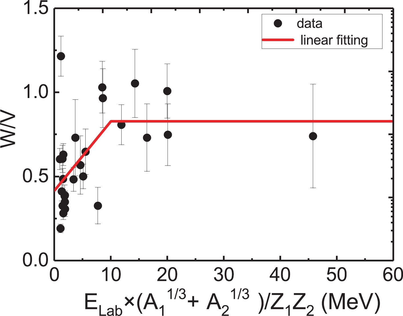
Figure 4. (color online) Value of
$W/V$ versus${{E}}_{\rm{lab}}\times(A_1^{1/3}+A_2^{1/3})/Z_1Z_2$ . The dots represent the value for each system.$W/V$ decreases sharply when${{E}}_{\rm{lab}}\times(A_1^{1/3}+A_2^{1/3})/Z_1Z_2$ $<$ 10 and remains relatively stable when${{E}}_{\rm{lab}}\times(A_1^{1/3}+A_2^{1/3})/Z_1Z_2$ $\geqslant$ 10. The red line is a simple linear fit to describe the behavior of$W/V$ .4) The volume integral is considered to be a reliable physical quantity for describing the total strength of a potential [26, 27]; it is expressed as
$ J_V = \frac{4\pi}{A_1\ A_2} \int V_n(r)r^2\ {\rm d}r. $

(5) The SPP can describe the realistic potential successfully [12, 28], and it is adopted to calculate the volume integrals for every system in this work. The depth and radius parameters are determined by requiring that they satisfy Eq. (4) [with a determined by Eq. (3)] and their corresponding
$ J_V $ -values are the same as those given by the SPP systematics. The calculated volume integrals and depth and radius parameters are shown in Table 2 and in Figs. 5, 6, and 7, respectively.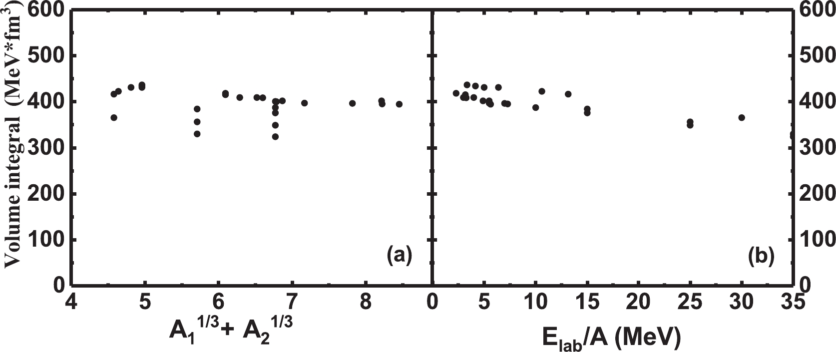
Figure 5. Volume integrals versus
$(A_1^{1/3}+A_2^{1/3})$ (a) and incident energy (b). The volume integrals of the different systems are similar, and they decrease slightly as the incident energy increases.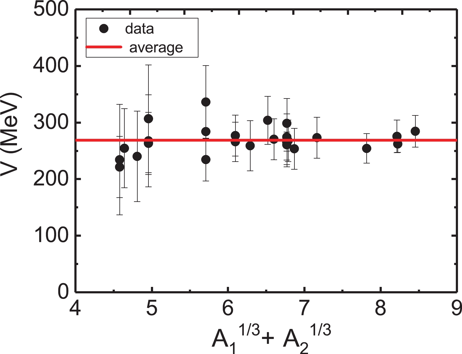
Figure 6. (color online) Depth of the real part determined by
$const1$ and the volume integral. The values show system independence.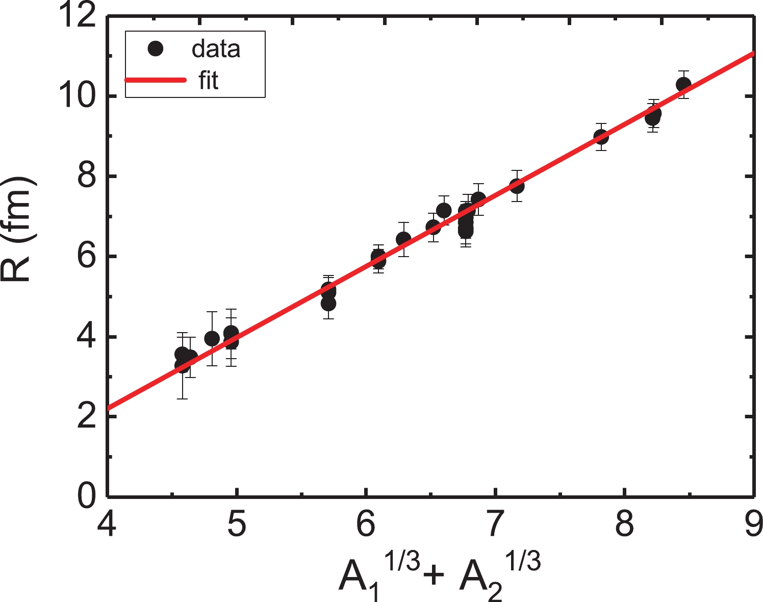
Figure 7. (color online) Radius parameters determined by
$const1$ and the volume integral. There is a strong linear relationship between the radius parameter and$(A_1^{1/3}+A_2^{1/3})$ .In Fig. 5, it is evident that the volume integrals of the various systems are relatively close and that they decrease slightly as the incident energy increases. The depth of the real part of each system exhibits system independence and an insignificant energy dependence. The variations in the real depth induced by the incident energy are less than 10 MeV for all systems, and the theoretical angular distributions rarely change. An average value of 268.7
$ \pm $ 24.1 MeV is thus adopted for the depth, as shown in Fig. 6. The analysis of the radius parameters is shown in Fig. 7, where we find that the linear expression with$ A_1^{1/3}+A_2^{1/3} $ describes the trend of the radius parameter very well. The expressions of the depth and radius parameters are shown in Eq. (6). Using the expressions for the optical potential parameters in Eq. (3) and Eq. (6),$ const1 $ and$ const2 $ can be calculated for all systems, the results of which are plotted in Fig. 8.
Figure 8. (color online) Values of
$const1$ (a) and$const2$ (b) in Eq. (4) versus$A_1^{1/3}+A_2^{1/3}$ for each reaction. The values of$const1$ and$const2$ increase sharply as$A_1^{1/3}+A_2^{1/3}$ increases. The dots with error bars represent the data, and the red triangles denote the results calculated by adopting the formulas in Eqs. (3) and (6). The theoretical points are connected by the red curves to describe the trend of$const1$ and$const2.$ $ \begin{aligned}[b] V =& (268.7 \pm 24.1) \ \ {({\rm{MeV}}),}\\ W/V =& \left\{ \begin{array}{l} 0.0416\times EDRP+0.4124 \ \ \ EDRP<10, \\ 0.8284\ \ \ \ \ \ EDRP\geqslant10, \\ \end{array}\right.\\ R_V =& R_W = (1.772\pm 0.039)\times (A_1^{1/3}+A_2^{1/3})\\ &\ \ \ \ \ \ \ \ \ \ \ \ -(4.881\pm 0.256)\ \ {\rm{(fm),}}\\ EDRP =& E_{\rm{lab}}\times(A_1^{1/3}+A_2^{1/3})/Z_1Z_2. \end{aligned} $

(6) -
The systematics of the Woods-Saxon parameters extracted in the present work are checked using various elastic scattering data. The systematics derived by Wang et al. [13, 14] and Xu et al. [15] are also employed to calculate angular distributions for comparison. The results can be seen in Figs. 9-13.
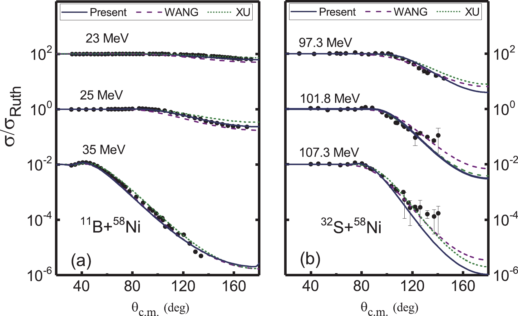
Figure 9. (color online) Comparison of the differential cross sections from the experimental data and theoretical calculations. The solid curves are calculated with the systematics summarized in this work. The results of Xu et al. [15] (dashed line) and Wang et al. [13, 14] (short dashed line) are also shown. The different data sets are offset by factors of 104. The experimental data are from Refs. [29-33].

The current systematic potential parameters can reproduce the experimental data very well, not only for the elastic scattering induced by 11B, 12C , and 16O but also for other systems, such as 28Si, 32S, and 40Ca + nucleus. For most of the systems, our results yield a description similar to those of Xu et al. [15] and Wang et al. [13, 14]. For some scattering systems, especially for relatively light systems, such as 12C + 12C at 158.8 MeV and 360 MeV (Fig. 9), 12C + 13C at 127.2 MeV (Fig. 9), and 11B + 58Ni at 25 MeV (Fig. 13), the present systematic results are even better.
-
The elastic scattering angular distributions of 11B, 12C, and 16O + heavy-ions at incident energies between 2.3 and 35 A MeV were fitted with the six-parameter Woods-Saxon potential. We obtained
$ \chi^{2} $ for each calculation to find the best-fit parameter combinations. The diffuseness parameter was determined first, followed by the relationship with$ A_1^{1/3}+A_2^{1/3} $ . Using the formula for the diffuseness parameter, the ratio of the imaginary depth to the real depth was obtained, and the correlation between the depth and radius parameters was found. With the limitation of the volume integrals calculated using SPP, the values of the depth and radius parameters of various systems were determined. Because the real depth exhibits system independence and ignorable energy dependence, the average value was adopted for all systems. The values of$ W/V $ show strong energy dependence when the incident energy is below or around the Coulomb barrier. The radius parameters have a strong linear relationship with$ A_1^{1/3}+A_2^{1/3} $ , and the expression was fitted. The systematic potential parameters summarized in the present work reproduce various interaction systems induced by 11B, 12C, and 16O well and can also reproduce elastic scattering induced by other heavy ions, such as 28Si, 32S, and 40Ca + nucleus.Nevertheless, the present work is not fully satisfactory. For some heavy systems, such as 40Ca+96Zr at incident energies of 152 MeV [52], our result is not quite satisfactory. More detailed studies are needed to analyze the relevant parameters, such as isospin.
It is difficult to directly extract the optical potential between some heavy ions, especially those between unstable nuclei. Nonetheless, the systematic study of optical potential parameters in these situations is particularly important. Although there have been some studies on the nuclear-nuclear interaction potential between heavy ions, these works have system limitations; that is, some systems are reproduced well, while others are not. Therefore, further research in this area is still needed.
Systematic study of the Woods-Saxon potential parametersbetween heavy-ions
- Received Date: 2020-06-30
- Available Online: 2021-05-15
Abstract: Experimental elastic scattering angular distributions of 11B, 12C, and 16O + heavy-ions are used to study the Woods-Saxon potential parameters. Best fitted values of the diffuseness parameters are found for each system, and a linear relationship is expressed between the diffuseness parameters and


 DownLoad: