


 Abstract
 HTML
HTML Reference
 Related
 PDF
PDF


-
Since the flavor changing neutral current process (FCNC)
$ b\to s\gamma $ originates only from loop diagrams, it is very sensitive to new physics beyond the Standard Model (SM). The updated average branching ratio for inclusive$ \bar{B}\rightarrow X_s\gamma $ is [1]$ \begin{array}{l} BR(\bar{B}\rightarrow X_s\gamma)_{\rm exp} = (3.32\pm0.15)\times10^{-4}, \end{array} $

(1) and the SM prediction at next-next-to-leading order (NNLO) is [2-4]
$ \begin{array}{l} BR(\bar{B}\rightarrow X_s\gamma)_{\rm SM} = (3.40\pm0.17)\times10^{-4}. \end{array} $

(2) Though the deviation of the SM prediction from experimental results has been almost eliminated in the past few years, it is helpful to constrain parameters of new physics.
The discovery of the Higgs boson at the Large Hadron Collider (LHC) has made the SM the most successful theory in particle physics to date. However, because of the hierarchy problem and the missing gravitational interaction, it is believed that the SM is just an effective approximation of a more fundamental theory at a higher scale. Among the various proposed extensions of the SM, supersymmetric models have been studied for decades.
As the simplest extension, the Minimal Supersymmetric Standard Model (MSSM) [5-7] solves the hierarchy problem as well as the instability of the Higgs boson by introducing a superpartner for each SM particle. The lightest supersymmetric particle (LSP) within this framework also provides candidates for dark matter as weakly interacting massive particles (WIMPs). However, the MSSM cannot naturally generate the tiny neutrino mass which is needed to explain the observation of neutrino oscillation. To acquire neutrino masses, heavy Majorana neutrinos are introduced in the seesaw mechanism, which implies that the lepton numbers are broken. Besides, the baryon numbers are also expected to be broken because of the matter-antimatter asymmetry in the universe. The authors of Refs. [8, 9] have presented the so-called BLMSSM model, in which the baryon and lepton number are locally gauged and spontaneously broken at TeV scale. The experimental bounds on proton decay lifetime are the main motivation of the great desert hypothesis. In the BLMSSM, proton decay can be avoided with discrete symmetries called matter parity and R-parity [10]
To describe the symmetries of baryon and lepton numbers, the gauge group is enlarged to
$ SU(3)_C \otimes SU(2)_L \otimes $ $ U(1)_Y \otimes U(1)_B \otimes U(1)_L $ . Corrections to various observations can then be induced from new gauge boson and exotic fields within this scenario. In Ref. [11], corrections to the anomalous magnetic moment from one-loop diagrams and two-loop Barr-Zee type diagrams are investigated with an effective Lagrangian method. One-loop contributions to the$ c(t) $ electric dipole moment in the CP-violating BLMSSM are presented in Ref. [12]. To account for the experimental data on the Higgs boson, the authors of Ref. [13] have studied the signals of$ h\to\gamma\gamma $ and$ h\to VV^*(V = Z,W) $ with a 125 GeV Higgs. In this work, we use the branching ratio to constrain the parameters. Furthermore, we present the corrections to CP-violation of$ b\to s\gamma $ due to new parameters introduced in this model.This paper is organized as follows. In Section II, we briefly introduce the construction of the BLMSSM and the interactions we need for our caculation. After that, we present the one-loop corrections to the branching ratio and CP-violation with the effective Lagrangian method in Section III. Numerical results are discussed in Section IV and the conclusions are given in Section V.
-
The BLMSSM is based on the gauge symmetry
$ SU(3)_C \otimes SU(2)_L \otimes U(1)_Y \otimes U(1)_B \otimes U(1)_L $ . In order to cancel the anomalies of baryon number (B), the exotic quarks$ \hat{Q}_4 \sim (3 , 2 , 1/6 , B_4 , 0),\; \hat{U}^c_4 \sim (\bar{3} , 1 , -2/3, - B_4, 0 ), \; \hat{D}^c_4 \sim (\bar{3} , 1 , 1/3 , $ $ -B_4 , 0 ), \; \hat{Q}_5^c \sim (\bar{3} , 2 , -1/6, -(1+B_4), 0 ),\; \hat{U}_5 \sim (3, 1 , 2/3 , 1 + B_4, 0 ),$ $ \hat{D}_5 \sim (3, 1 , -1/3 , 1 + B_4, 0) $ are introduced. Baryon number is broken spontaneously after the Higgs superfields$ \hat{\Phi}_B \sim $ $ ( 1 , 1 , 0 , 1 , 0 ), \hat{\varphi}_B \sim ( 1 , 1 , 0 , -1 , 0 ) $ acquire nonzero vacuum expectation values (VEVs). To deal with the anomalies of lepton number (L), the exotic leptons$ \hat{L}_4 \sim ( 1 , 2 , -1/2 , $ $ 0 , L_4),\; \hat{E}^c_4 \sim ( 1 , 1 , 1 , 0 , -L_4), \;\hat{N}^c_4 \sim ( 1 , 1 , 0 , 0 , -L_4),\; \hat{L}_5^c \sim ( 1 , 2 , 1/2 , $ $ 0 , -(3 + L_4)),\; \hat{E}_5 \sim ( 1 , 1 , -1 , 0 , 3 + L_4), \; \hat{N}_5 \sim ( 1 , 1 , 0 , 0 , 3 + L_4) $ are introduced, and$ \hat{\Phi}_L \sim ( 1 , 1 , 0 , 0 , -2 ), \hat{\varphi}_L \sim ( 1 , 1 , 0 , 0 , 2) $ are responsible for the breaking of lepton number [9]. The superfields$ \hat{X} \sim ( 1 , 1 , 0 ,2/3 + B_4, 0 ), \hat{X'} \sim ( 1 , 1 , 0 , -(2/3 + $ $ B_4), 0) $ , which mediate the decay of exotic quarks, are added in this model to avoid their stability.Given the superfields above, one can construct the superpotential as
$ \begin{array}{l} {\cal W}_{{\rm BLMSSM}} = {\cal W}_{{\rm MSSM}}+{\cal W}_{B}+{\cal W}_{L}+{\cal W}_{X}, \end{array} $

(3) where
$ {\cal W}_{{\rm MSSM}} $ indicates the superpotential of MSSM, and$ \begin{aligned}[b] {\cal W}_{B}=& \lambda_{Q}\hat{Q}_{4}\hat{Q}_{5}^c\hat{\Phi}_{B}+\lambda_{U}\hat{U}_{4}^c\hat{U}_{5} \hat{\varphi}_{B}+\lambda_{_D}\hat{D}_{4}^c\hat{D}_{5}\hat{\varphi}_{B}+\mu_{B}\hat{\Phi}_{B}\hat{\varphi}_{B} \\ & +Y_{{u_4}}\hat{Q}_{4}\hat{H}_{u}\hat{U}_{4}^c+Y_{{d_4}}\hat{Q}_{4}\hat{H}_{d}\hat{D}_{4}^c+Y_{{u_5}}\hat{Q}_{5}^c\hat{H}_{d}\hat{U}_{5}+Y_{{d_5}}\hat{Q}_{5}^c\hat{H}_{u}\hat{D}_{5}, \\ {\cal W}_{L}=& Y_{{e_4}}\hat{L}_{4}\hat{H}_{d}\hat{E}_{4}^c+Y_{{\nu_4}}\hat{L}_{4}\hat{H}_{u}\hat{N}_{4}^c +Y_{{e_5}}\hat{L}_{5}^c\hat{H}_{u}\hat{E}_{5}+Y_{{\nu_5}}\hat{L}_{5}^c\hat{H}_{d}\hat{N}_{5} \\ & +Y_{\nu}\hat{L}\hat{H}_{u}\hat{N}^c+\lambda_{{N^c}}\hat{N}^c\hat{N}^c\hat{\varphi}_{L} +\mu_{L}\hat{\Phi}_{L}\hat{\varphi}_{L}\;, \\ {\cal W}_{X}=& \lambda_1\hat{Q}\hat{Q}_{5}^c\hat{X}+\lambda_2\hat{U}^c\hat{U}_{5}\hat{X}^\prime +\lambda_3\hat{D}^c\hat{D}_{5}\hat{X}^\prime+\mu_{X}\hat{X}\hat{X}^\prime\;. \end{aligned} $

(4) The soft breaking terms are given by
$ \begin{aligned}[b] {\cal L}_{{\rm soft}} =& {\cal L}_{{\rm soft}}^{\rm MSSM}-(m_{\tilde{N}^c}^2)_{{IJ}}\tilde{N}_I^{c*}\tilde{N}_J^c -m_{{\tilde{Q}_4}}^2\tilde{Q}_{4}^\dagger \tilde{Q}_{4}-m_{{\tilde{U}_4}}^2\tilde{U}_{4}^{c*}\tilde{U}_{4}^c -m_{{\tilde{D}_4}}^2\tilde{D}_{4}^{c*}\tilde{D}_{4}^c -m_{{\tilde{Q}_5}}^2\tilde{Q}_{5}^{c\dagger}\tilde{Q}_{5}^c -m_{{\tilde{U}_5}}^2\tilde{U}_{5}^*\tilde{U}_{5} -m_{{\tilde{D}_5}}^2\tilde{D}_{5}^*\tilde{D}_{5}-m_{{\tilde{L}_4}}^2\tilde{L}_{4}^\dagger \tilde{L}_{4} -M_{{\tilde{\nu}_4}}^2\tilde{\nu}_{4}^{c*}\tilde{\nu}_{4}^c\\ &-m_{{\tilde{E}4}}^2\tilde{e}_{4}^{c*}\tilde{e}_{4}^c -m_{{\tilde{L}_5}}^2\tilde{L}_{5}^{c\dagger}\tilde{L}_{5}^c -M_{{\tilde{\nu}_5}}^2\tilde{\nu}_{5}^*\tilde{\nu}_{5}-m_{{\tilde{E}_5}}^2\tilde{e}_{5}^*\tilde{e}_{5} -m_{{\Phi_{B}}}^2\Phi_{B}^*\Phi_{B}-m_{{\varphi_{B}}}^2\varphi_{B}^*\varphi_{B} -m_{{\Phi_{L}}}^2\Phi_{L}^*\Phi_{L} -m_{{\varphi_{L}}}^2\varphi_{L}^*\varphi_{L}-(m_{B}\lambda_{B}\lambda_{B} +m_{L}\lambda_{L}\lambda_{L}+{\rm h.c.}) \\ & +\Big\{A_{{u_4}}Y_{{u_4}}\tilde{Q}_{4}H_{u}\tilde{U}_{4}^c+A_{{d_4}}Y_{{d_4}}\tilde{Q}_{4}H_{d}\tilde{D}_{4}^c +A_{{u_5}}Y_{{u_5}}\tilde{Q}_{5}^cH_{d}\tilde{U}_{5}+A_{{d_5}}Y_{{d_5}}\tilde{Q}_{5}^cH_{u}\tilde{D}_{5} +A_{{BQ}}\lambda_{Q}\tilde{Q}_{4}\tilde{Q}_{5}^c\Phi_{B}+A_{{BU}}\lambda_{U}\tilde{U}_{4}^c\tilde{U}_{5}\varphi_{B} \\ &+A_{{BD}}\lambda_{D}\tilde{D}_{4}^c\tilde{D}_{5}\varphi_{B} +B_{B}\mu_{B}\Phi_{B}\varphi_{B} +{\rm h.c.}\Big\} +\Big\{A_{e_4}Y_{{e_4}}\tilde{L}_{4}H_{d}\tilde{E}_{4}^c+A_{{N_4}}Y_{{N_4}}\tilde{L}_{4}H_{u}\tilde{N}_{4}^c +A_{{e_5}}Y_{{e_5}}\tilde{L}_{5}^cH_{u}\tilde{E}_{5}+A_{{N_5}}Y_{{\nu_5}}\tilde{L}_{5}^cH_{d}\tilde{N}_{5}\\ & +A_{N}Y_{N}\tilde{L}H_{u}\tilde{N}^c+A_{{N^c}}\lambda_{{N^c}}\tilde{N}^c\tilde{N}^c\varphi_{L} +B_{L}\mu_{L}\Phi_{L}\varphi_{L}+{\rm h.c.}\Big\} +\Big\{A_1\lambda_1\tilde{Q}\tilde{Q}_{5}^cX+A_2\lambda_2\tilde{U}^c\tilde{U}_{5}X^\prime +A_3\lambda_3\tilde{D}^c\tilde{D}_{5}X^\prime+B_{X}\mu_{X}XX^\prime+{\rm h.c.}\Big\}\;. \end{aligned} $ 
(5) The first term
$ {\cal L}_{{\rm soft}}^{\rm MSSM} $ denotes the soft breaking terms of the MSSM. To break the gauge symmetry from$ SU(3)_C \otimes SU(2)_L \otimes U(1)_Y \otimes U(1)_B \otimes U(1)_L $ to electromagnetic symmetry$ U(1)_e $ , nonzero VEVs$ v_u, v_d $ and$ v_B, \bar{v}_B, v_L,\bar{v}_L $ are allocated to the$ SU(2)_L $ doublets$ H_u, H_d $ and$ SU(2)_L $ singlets$ \Phi_B, \varphi_B, \Phi_L, \varphi_L $ :$ \begin{aligned}[b] H_u =& \left(\begin{array}{c} H_u^+\\ (v_u+H_u^0+{\rm i}P_u^0)/\sqrt{2} \end{array}\right),\end{aligned} $

$ \begin{aligned}[b] H_u = &\left(\begin{array}{c} (v_d+H_d^0+{\rm i}P_d^0)/\sqrt{2}\\ H_d^- \end{array}\right),\\ \Phi_B =& (v_B+\Phi_B^0+{\rm i}P_B^0)/\sqrt{2},\\ \varphi_B =& (\bar{v}_B+\varphi_B^0+{\rm i}\bar{P}_B^0)/\sqrt{2},\\ \Phi_L = &(v_L+\Phi_L^0+{\rm i}P_L^0)/\sqrt{2},\\ \varphi_L =& (\bar{v}_L+\varphi_L^0+{\rm i}\bar{P}_L^0)/\sqrt{2}. \end{aligned} $

(6) Here we take the notation
$ \tan\beta = v_u/v_d,\; \tan\beta_B = \bar{v}_B/v_B $ and$ \tan\beta_L = \bar{v}_L/v_L $ . After spontaneous breaking and unitary transformation from interactive eigenstate to mass eigenstate, one can extract the Feynman rules and mass spectra in the BLMSSM. The mass matrices of the particles that mediate the one-loop process$ b\to s\gamma $ can be found in Ref. [14]. The Feynman rules that we need can be extracted from the following terms, where all the repeated indices of generation should be summed over:$ \begin{aligned}[b] {\cal{L}}_{H^\pm du} =& \Bigg(-Y_d^IZ_H^{1i}P_L+Y_u^JZ_H^{2i}P_R\Bigg)K^{JI*}\bar{d}^Iu^JH_i^-,\\ {\cal{L}}_{\tilde{D} \chi^0d} =& \Bigg[\Bigg(\frac{-e}{\sqrt{2}s_Wc_W}Z_D^{Ii} (\frac{1}{3}Z_N^{1j}s_W-Z_N^{2j}c_W)+Y_d^IZ_D^{(I+3)i}Z_N^{3j}\Bigg)P_L\\ & +\Bigg(\frac{-e\sqrt{2}}{3c_W}Z_D^{(I+3)i}Z_N^{1j*}+Y_d^IZ_D^{Ii}Z_N^{3j*} \Bigg)P_R\Bigg] \bar{\chi}^0_jd^I\tilde{D}^+_i,\\ {\cal{L}}_{\tilde{D}\chi_B^0d} =& \frac{\sqrt{2}}{3}g_B\Bigg(Z_{N_B}^{1j}Z_D^{Ii}P_L +Z_{N_B}^{1j*}Z_D^{(I+3)i}P_R\Bigg)\bar{\chi}_{B_j}^0d^I\tilde{D}^+,\\ {\cal{L}}_{\tilde{U}\chi^-d} =& \Bigg[\Bigg(\frac{-e}{s_W}Z_U^{Ji*}Z_+^{1j} +Y_u^JZ_U^{(J+3)i*}Z_+^{2j}\Bigg)P_L-Y_d^IZ_U^{Ji*}Z_-^{2j*}P_R\Bigg]\\&\times K^{JI}\bar{\chi}^-d\tilde{U}^-,\\ {\cal{L}}_{Xb^\prime d} =& \Bigg[\lambda_{1}(W_b^{\dagger})_{j1}(Z_X)_{1k}P_L -\lambda_{3}^*(U_b^{\dagger})_{j2}(Z_X)_{2k}P_R\Bigg]\bar{b}^\prime_jd^IX_k,\\ {\cal {L}}_{\tilde{b}^\prime\tilde{X} d} =& -\Bigg[\lambda_1(W_{\tilde{b}^\prime}^*)_{3\rho}P_L +\lambda_3^*(W_{\tilde{b}^\prime})_{4\rho}P_R\Bigg] \bar{\tilde{X}}d^I\tilde{b}^\prime_\rho,\\ {\cal {L}}_{\tilde{D}\Lambda_G d} = &g_3\sqrt{2}Y_{\alpha\beta}^a \Bigg(-Z_D^{Ii}P_L+Z_D^{(I+3)i}P_R\Bigg)\bar{\Lambda}_G^a d_\beta^I\tilde{D}^+_{i\alpha}. \end{aligned} $

(7) The interactions from the MSSM are collected from Ref. [7] for completeness, and the Feynman gauge is used in our derivation to stay consistent with the MSSM sector.
-
The flavor transition process
$ b\rightarrow s\gamma $ can be described by the effective Hamiltonian at scale$ \mu = O(m_b) $ as follows [15-17]:$ \begin{aligned}[b] {\cal {H}}_{\rm eff}(b\to s\gamma) =& -\frac{4G_F}{\sqrt{2}}V_{ts}^*V_{tb} \Bigg[C_1Q_1^c+C_2Q_2^c\\&+\sum_{i = 3}^6C_iQ_i+\sum_{i = 7}^8(C_iQ_i+\tilde{C}_i\tilde{Q}_i)\Bigg], \end{aligned} $

(8) and the operators are given by Ref. [18-22]:
$ \begin{aligned}[b] {\cal{O}}_1^c =& (\bar{s}_L\gamma_\mu T^ab_L)(\bar{c}_L\gamma^\mu T^ab_L),\\ {\cal{O}}_2^c =& (\bar{s}_L\gamma_\mu b_L)(\bar{c}_L\gamma^\mu T^a b_L),\\ {\cal{O}}_3 =& (\bar{s}_L\gamma_\mu b_L)\sum_q(\bar{q}\gamma^\mu q), \end{aligned} $

$ \begin{aligned}[b]{\cal{O}}_4 =& (\bar{s}_L\gamma_\mu T^ab_L)\sum_q(\bar{q}\gamma^\mu T^a q),\\ {\cal{O}}_5 =& (\bar{s}_L\gamma_\mu \gamma_\nu\gamma_\rho b_L)\sum_q(\bar{q}\gamma^\mu \gamma^\mu \gamma^\nu\gamma^\rho q),\\ {\cal{O}}_6 =& (\bar{s}_L\gamma_\mu \gamma_\nu\gamma_\rho T^a b_L)\sum_q(\bar{q}\gamma^\mu \gamma^\mu \gamma^\nu\gamma^\rho T^a q),\\ {\cal{O}}_7 = & e/g_s^2m_b(\bar{s}_L\sigma_{\mu\nu}b_R)F^{\mu\nu},\\ {\cal{O}}_8 =& 1/g_s^2m_b(\bar{s}_L\sigma_{\mu\nu}T^ab_R)G^{a,\mu\nu},\\ \tilde{{\cal{O}}}_7 =& e/g_s^2m_b(\bar{s}_R\sigma_{\mu\nu}b_L)F^{\mu\nu},\\ \tilde{{\cal{O}}}_8 =& 1/g_s^2m_b(\bar{s}_R\sigma_{\mu\nu}T^ab_L)G^{a,\mu\nu}. \end{aligned} $

(9) The coefficients of these operators can be extracted from Feynman amplitudes that originate from the diagrams considered. Actually only the coefficients of
$ {\cal{O}}_{7,8} $ and$ \tilde{{\cal{O}}}_{7,8} $ are needed if we adopt the branching ratio formula presented in Ref. [15]:$ \begin{aligned}[textbf{}] BR(\bar{B}\rightarrow X_s\gamma)_{NP} =& 10^{-4}\times\Bigg\{(3.32\pm0.15)\\&+\frac{16\pi^2a_{77}}{\alpha_s^2(\mu_b)}\big[|C_{7,NP}(\mu_{EW})|^2+|\tilde{C}_{7,NP}(\mu_{EW})|^2\big]\\ & +\frac{16\pi^2a_{88}}{\alpha_s^2(\mu_b)}\big[|C_{8,NP}(\mu_{EW})|^2+|\tilde{C}_{8,NP}(\mu_{EW})|^2\big]\\& +\frac{ 4\pi}{\alpha_s(\mu_b)}\rm{Re}\big[a_7C_{7,NP}(\mu_{EW})+a_8C_{8,NP}(\mu_{EW})\big.\\& +\big.\frac{ 4\pi a_{78}}{\alpha_s(\mu_b)}\big(C_{7,NP}(\mu_{EW})C_{8,NP}(\mu_{EW})\\&+\tilde{C}_{7,NP}(\mu_{EW})\tilde{C}_{8,NP}(\mu_{EW})\big)\big]\Bigg\}, \end{aligned} $

(10) where the first term is the SM prediction. The other terms come from new physics in which
$ C_{7,NP}(\mu_{EW}) $ ,$ C_{8,NP}(\mu_{EW}) $ ,$ \tilde{C}_{7,NP}(\mu_{EW}) $ and$ \tilde{C}_{8,NP}(\mu_{EW}) $ indicate Wilson coefficients at the electroweak scale. One advantage of this expression is that they do not have to be evolved down to hadronic scale$ \mu\sim m_b $ , as the effect of evolution has already been involved in the coefficients$ a_{7,8,77,88,78} $ . The numerical values of these coefficients are given in Table 1.$a_7$ 

$a_8$ 

$a_{77}$ 

$a_{88}$ 

$a_{78}$ 

$-7.184+0.612{\rm i}$ 

$-2.225-0.557{\rm{i}}$ 

4.743 0.789 2.454−0.884i Table 1. Numerical values for the coefficients
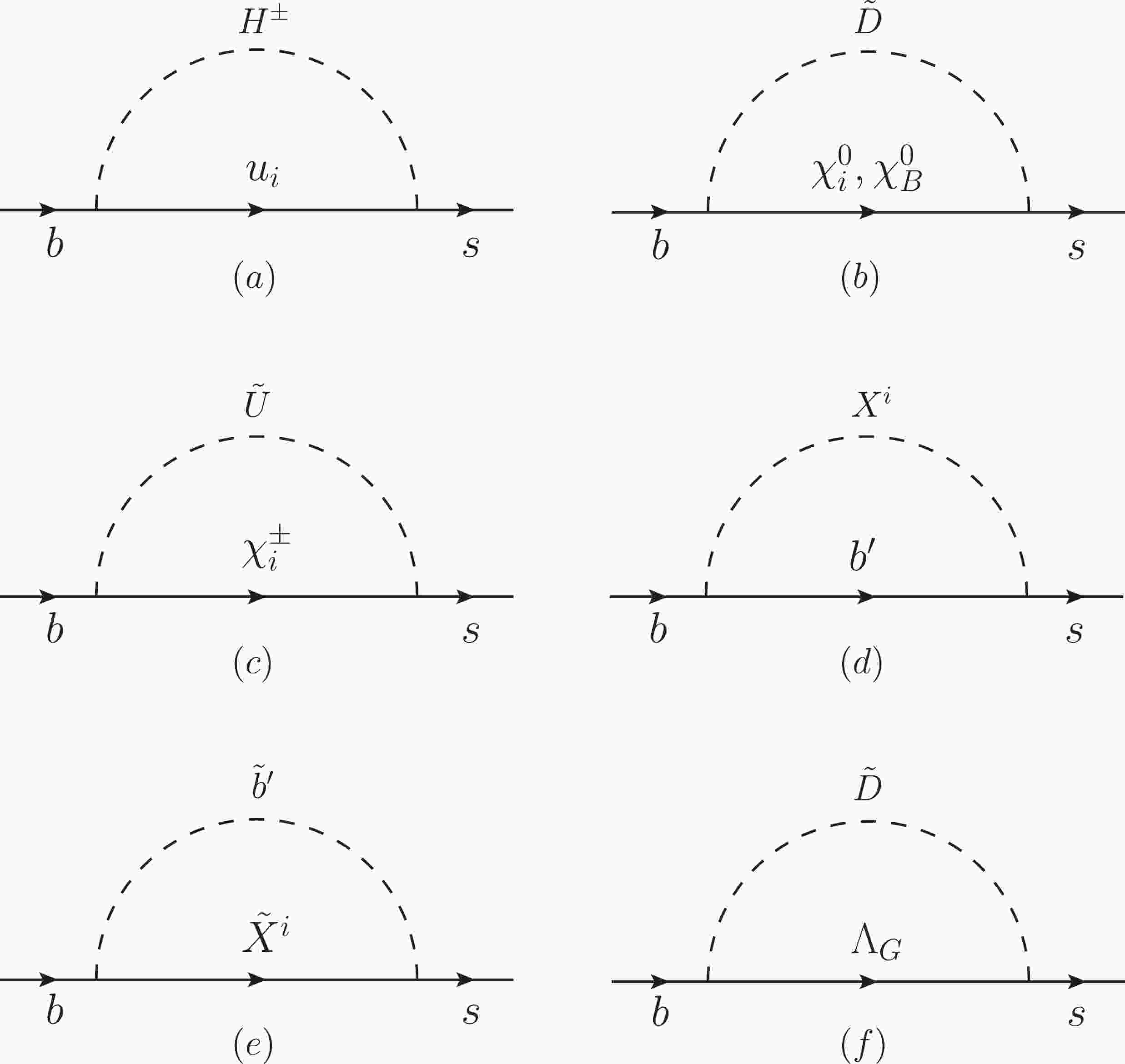
$a_{7,8,77,88,78}$ at electroweak scale.To obtain the new physics corrections in the BLMSSM, we investigate the one-loop diagrams shown in Fig. 1. Photons should be attached to all inner lines with electric charge to complete the diagrams of
$ b\to s\gamma $ that contribute to$ {\cal{O}}_7 $ and$ \tilde{{\cal{O}}}_7 $ . Similarly, diagrams of$ b\to sg $ can be completed with gluons attached to all the inner lines with color charge, and$ {\cal{O}}_8 $ and$ \tilde{{\cal{O}}}_8 $ originate from these processes.
Figure 1. One-loop Feynman diagrams for
$b\to s$ . The inner-line particles$\chi_B^0, X$ denote baryon neutralinos and a new scalar particle introduced in the BLMSSM.$b'$ and$\tilde{b}'$ are exotic quarks and squarks respectively. The photon and gluon can be attached in all possible ways.The so-called flavor-changing self-energy diagrams in which photos or gluons are attached to external b or s quarks are not included in our calculations. As studied in Refs. [23-25], the contributions from those self-energy diagrams vanish when one of the external legs is on its mass shell. To preserve the Ward-Takahashi identity during the renormalization of
$ \bar{s}bg $ and$ \bar{s}b\gamma $ vertices, one can always impose the renormalized self-energies as zero, as both b and s are on mass shell.In detail, we attach a photon to the SM quark
$ u_i,(i = 1,2,3) $ or charged Higgs$ H^\pm $ in Fig. 1(a) to get a set of trigonal diagrams for$ b\to s\gamma $ , while the gluon can only be attached to up-type quarks$ u_i $ to form a specific diagram of$ b\to sg $ . To give a complete correction originating from Fig. 1(a), contributions from all generations of$ u_i $ and Higgs should be summed over. From the amplitudes of these diagrams, one can extract the Wilson coefficients of electric- and chromomagnetic-dipole operators$ {\cal{O}}_{7} $ and$ \tilde{{\cal{O}}}_{7} $ at electroweak scale,$ \begin{aligned}[b] \frac{G_{\rm F}}{\sqrt{2}}C_{7\gamma}^a(\Lambda) =& -{\rm i}\Lambda^{-2}(V^*_{ts}V_{tb})^{-1} \left\{ (\eta^L_{H^\pm})_{su_i}^\dagger (\eta^L_{H^\pm})_{u_ib}F_{1,\gamma}^{(a)}(x_{u_i},x_{H^\pm})\right.\\ & \left.+\frac{m_f}{m_b}(\eta^L_{H^\pm})_{su_i}^\dagger (\eta^R_{H^\pm})_{u_ib}F_{2,\gamma}^{(a)}(x_{u_i},x_{H^\pm})\right\},\\ \frac{G_{\rm F}}{\sqrt{2}}\tilde{C}_{7\gamma}^a(\Lambda) = & \frac{G_{\rm F}}{\sqrt{2}}C_{7\gamma}^a(\Lambda)\big(\eta^L_{H^\pm}\leftrightarrow\eta^R_{H^\pm}\big), \\[-5pt] \end{aligned} $

(11) where
$ x_i = m_i^2/\mu_{EW}^2 $ . The concrete expressions for the relevant couplings have already been given in the previous section. To be clear, the absence of divergences in the Wilson coefficients associated with one-loop triangle diagrams can be verified by expanding all the propagators in the power of$ 1/(q^2-m^2_{f,S}) $ , where$ q $ denotes the loop momentum. It can found that the order of q that appear in the denominators is always higher than those in the numerators. Thus, we do not have to deal with divergences during our evaluation. The form factors in Eq. (11) can be written as:$ \begin{aligned}[b] F_{1,\gamma}^{(a)}(x,y) =& \Bigg[\frac{1}{72}\frac{\partial^3\varrho_{_{3,1}}}{\partial y^3} +\frac{1}{24}\frac{\partial^2\varrho_{_{2,1}}}{\partial y^2} -\frac{1}{ 6}\frac{\partial\varrho_{_{1,1}}}{\partial y}\Bigg](x,y),\\ F_{2,\gamma}^{(a)}(x,y) =& \Bigg[\frac{1}{12}\frac{\partial^2\varrho_{_{2,1}}}{\partial y^2} -\frac{1}{6}\frac{\partial\varrho_{_{1,1}}}{\partial y} -\frac{1}{3}\frac{\partial\varrho_{_{1,1}}}{\partial x}\Bigg](x,y), \end{aligned} $

(12) where the function
$ \varrho_{m,n}(x,y) $ is defined as:$ \varrho_{_{m,n}}(x,y) = {x^m\ln^nx-y^m\ln^ny\over x-y}. $

(13) Corrections from all the other diagrams to
$ C_{7\gamma} $ and$ \tilde{C}_{7\gamma} $ can be obtained similarly. In Fig. 1(b), the photon can only be attached to the charged −1/3 squark$ \tilde{D} $ . We present contributions from both neutralinos$ \chi_i^0 $ and baryon neutralinos$ \chi_B^0 $ at electroweak scale as:$ \begin{aligned}[b] \frac{G_{\rm F}}{\sqrt{2}}C_{7\gamma}^b(\Lambda) =& -{\rm i}\Lambda^{-2}(V^*_{ts}V_{tb})^{-1} \Bigg\{ (\xi^L_{\chi_i^0})_{s\tilde{D}}^\dagger (\xi^L_{\chi_i^0})_{\tilde{D}b}F_{1,\gamma}^{(b)}(x_{\chi_i^0},x_{\tilde{D}}) \\&+\frac{m_f}{m_b}(\xi^L_{\chi_i^0})_{s\tilde{D}}^\dagger (\xi^R_{\chi_i^0})_{\tilde{D}b}F_{2,\gamma}^{(b)}(x_{\chi_i^0},x_{\tilde{D}})\\ & +(\xi^L_{\chi_B^0})_{s\tilde{D}}^\dagger (\xi^L_{\chi_B^0})_{\tilde{D}b}F_{1,\gamma}^{(b)}(x_{\chi_B^0},x_{\tilde{D}}) \\&+\frac{m_f}{m_b}(\xi^L_{\chi_B^0})_{s\tilde{D}}^\dagger (\xi^R_{\chi_B^0})_{\tilde{D}b}F_{2,\gamma}^{(b)}(x_{\chi_B^0},x_{\tilde{D}})\Bigg\},\\ \frac{G_{\rm F}}{\sqrt{2}}\tilde{C}_{7\gamma}^b(\Lambda) = & \frac{G_{\rm F}}{\sqrt{2}}C_{7\gamma}^b(\Lambda)\big(\xi^L_{\chi_i^0}\leftrightarrow\xi^R_{\chi_i^0}\;,\;\xi^L_{\chi_B^0}\leftrightarrow\xi^R_{\chi_B^0}\big). \end{aligned} $

(14) $ \begin{aligned}[b] F_{1,\gamma}^{(b)}(x,y) = & \Bigg[-\frac{1}{72}\frac{\partial^3\varrho_{_{3,1}}}{\partial^3y}+\frac{1}{24}\frac{\partial^2\varrho_{_{2,1}}}{\partial^2y}\Bigg](x,y),\\ F_{2,\gamma}^{(b)}(x,y) =& \Bigg[-\frac{1}{12}\frac{\partial^2\varrho_{_{2,1}}}{\partial^2y}+\frac{1}{6}\frac{\partial \varrho_{_{1,1}}}{\partial y}\Bigg](x,y). \end{aligned} $

(15) With the photon attached to the charged +2/3 squarks
$ \tilde{U} $ or chargino$ \chi^\pm_i $ in Fig. 1(c), the contributions to the Wilson coefficients read:$ \begin{aligned}[b] \frac{G_{\rm F}}{\sqrt{2}}C_{7\gamma}^c(\Lambda) =& -{\rm i}\Lambda^{-2}(V^*_{ts}V_{tb})^{-1} \Bigg\{ (\eta^L_{\tilde{U}})_{s\chi_i^{\pm}}^\dagger (\eta^L_{\tilde{U}})_{\chi_i^{\pm}b}F_{1,\gamma}^{(c)}(x_{\chi_i^{\pm}},x_{\tilde{U}}) \\&+\frac{m_f}{m_b}(\eta^L_{\tilde{U}})_{s\chi_i^{\pm}}^\dagger (\eta^R_{\tilde{U}})_{\chi_i^{\pm}b}F_{2,\gamma}^{(c)}(x_{\chi_i^{\pm}},x_{\tilde{U}})\Bigg\},\\ \frac{G_{\rm F}}{\sqrt{2}}\tilde{C}_{7\gamma}^c(\Lambda) =& \frac{G_{\rm F}}{\sqrt{2}}C_{7\gamma}^c(\Lambda)\big(\eta^L_{\tilde{U}}\leftrightarrow\eta^R_{\tilde{U}}\big), \end{aligned} $

(16) $ \begin{aligned}[b] F_{1,\gamma}^{(c)}(x,y) =& \Bigg[-\frac{1}{72}\frac{\partial^3\varrho_{_{3,1}}}{\partial^3y} +\frac{1}{ 6}\frac{\partial^2\varrho_{_{2,1}}}{\partial^2y} -\frac{1}{ 4}\frac{\partial \varrho_{_{1,1}}}{\partial y}\Bigg](x,y),\\ F_{2,\gamma}^{(c)}(x,y) = & \Bigg[-\frac{1}{12}\frac{\partial^2\varrho_{_{2,1}}}{\partial^2y} +\frac{1}{ 6}\frac{\partial\varrho_{_{1,1}}}{\partial y} -\frac{1}{ 2}\frac{\partial\varrho_{_{1,1}}}{\partial x}\Bigg](x,y). \end{aligned} $

(17) The intermediate particles in Fig. 1(d) are the exotic quarks
$ b^\prime $ with charge -1/3 and superfield$ X $ introduced in the BLMSSM. The contributions from this diagram are:$ \begin{aligned}[b] \frac{G_{\rm F}}{\sqrt{2}}C_{7\gamma}^d(\Lambda) =& -{\rm i}\Lambda^{-2}(V^*_{ts}V_{tb})^{-1} \Bigg\{ (\eta^L_{X^j})_{sb^\prime}^\dagger (\eta^L_{X^j})_{b^\prime b}F_{1,\gamma}^{(d)}(x_{b^\prime},x_{X^j}) \\&+\frac{m_f}{m_b}(\eta^L_{X^j})_{sb^\prime}^\dagger (\eta^R_{X^j})_{b^\prime b}F_{2,\gamma}^{(d)}(x_{b^\prime},x_{X^j})\Bigg\},\\ \frac{G_{\rm F}}{\sqrt{2}}\tilde{C}_{7\gamma}^d(\Lambda) =& \frac{G_F}{\sqrt{2}}C_{7\gamma}^d(\Lambda)\big(\eta^L_{X^j}\leftrightarrow\eta^R_{X^j}\big). \end{aligned} $

(18) Correspondingly, the corrections of exotic squarks
$ \tilde{b}^\prime $ with charge -1/3 and fermionic particle$ X $ can be obtained from Fig. 1(e):$ \begin{aligned}[b] \frac{G_{\rm F}}{\sqrt{2}}C_{7\gamma}^e(\Lambda) =& -{\rm i}\Lambda^{-2}(V^*_{ts}V_{tb})^{-1} \\&\times \Bigg\{ (\eta^L_{\tilde{b}^\prime})_{s\tilde{X}^j}^\dagger (\eta^L_{\tilde{b}^\prime})_{\tilde{X}^jb}F_{1,\gamma}^{(e)} (x_{\tilde{X}^j},x_{\tilde{b}^\prime}) \\& +\frac{m_f}{m_b}(\eta^L_{\tilde{b}^\prime})_{s\tilde{X}^j}^\dagger (\eta^R_{\tilde{b}^\prime})_{\tilde{X}^jb}F_{2,\gamma}^{(e)} (x_{\tilde{X}^j},x_{\tilde{b}^\prime})\Bigg\},\\ \frac{G_{\rm F}}{\sqrt{2}}\tilde{C}_{7\gamma}^e(\Lambda) =& \frac{G_{\rm F}}{\sqrt{2}}C_{7\gamma}^e(\Lambda)\big(\eta^L_{\tilde{b}^\prime}\leftrightarrow\eta^R_{\tilde{b}^\prime}\big), \end{aligned} $

(19) $ \begin{aligned}[b] F_{1,\gamma}^{(e)}(x,y) = & \Bigg[-\frac{1}{72}\frac{\partial^3\varrho_{_{3,1}}}{\partial^3y}+\frac{1}{24}\frac{\partial^2\varrho_{_{2,1}}}{\partial^2y}\Bigg](x,y),\\ F_{2,\gamma}^{(e)}(x,y) = & \Bigg[-\frac{1}{12}\frac{\partial^2\varrho_{_{2,1}}}{\partial^2y}+\frac{1}{ 6}\frac{\partial\varrho_{_{1,1}}}{\partial y}\Bigg](x,y). \end{aligned} $

(20) From Fig. 1(f), we obtain the corrections from gluinos
$ \Lambda_G $ in the MSSM, and the Wilson coefficients at$ \mu_{EW} $ are$ \begin{aligned}[b] \frac{G_{\rm F}}{\sqrt{2}}C_{7\gamma}^f(\Lambda) =& -{\rm i}\Lambda^{-2}(V^*_{ts}V_{tb})^{-1} \\&\times \Bigg\{ (\eta^L_{\tilde{D}})_{s\Lambda_G}^\dagger (\eta^L_{\tilde{D}})_{\Lambda_Gb}F_{1,\gamma}^{(f)}(x_{\Lambda_G},x_{\tilde{D}}) \\& +\frac{m_f}{m_b}(\eta^L_{\tilde{D}})_{s\Lambda_G}^\dagger (\eta^R_{\tilde{D}})_{\Lambda_Gb}F_{2,\gamma}^{(f)}(x_{\Lambda_G},x_{\tilde{D}})\Bigg\},\\ \frac{G_{\rm F}}{\sqrt{2}}\tilde{C}_{7\gamma}^f(\Lambda) =& \frac{G_{\rm F}}{\sqrt{2}}C_{7\gamma}^f(\Lambda)\big(\eta^L_{\tilde{D}}\leftrightarrow\eta^R_{\tilde{D}}\big), \end{aligned} $

(21) with
$ \begin{aligned}[b] F_{1,\gamma}^{(f)}(x,y) =& \Bigg[\frac{1}{24}\frac{\partial^3\varrho_{_{3,1}}}{\partial^3y}-\frac{1}{8}\frac{\partial^2\varrho_{_{2,1}}}{\partial^2y}\Bigg](x,y),\\ F_{2,\gamma}^{(f)}(x,y) = & \Bigg[\frac{1}{ 4}\frac{\partial^2\varrho_{_{2,1}}}{\partial^2y}-\frac{1}{2}\frac{\partial\varrho_{_{1,1}}}{\partial y}\Bigg](x,y). \end{aligned} $

(22) The corrections to
$ C_{8g} $ and$ \tilde{C}_{8g} $ at electroweak scale can be obtained by attaching the gluon to intermediate virtual particles with colors. For diagrams in Fig. 1, the gluon can be attached to SM up-type quarks$ u_i $ , MSSM squarks$ \tilde{U}, \tilde{D} $ , exotic quarks$ b^\prime $ with charge -1/3 and their supersymmetric partners$ \tilde{b}^\prime $ , and gluinos$ \Lambda_G $ . The Wilson coefficients at electroweak scale can be formulated as:$ \begin{aligned}[b] \frac{G_{\rm F}}{\sqrt{2}}C_{8G}^a(\Lambda) =& -{\rm i}\Lambda^{-2}(V^*_{ts}V_{tb})^{-1} \left\{ (\eta^L_{H^\pm})_{su_i}^\dagger (\eta^L_{H^\pm})_{u_ib}F_{1,g}^{(a)}(x_{u_i},x_{H^\pm}) +\frac{m_f}{m_b}(\eta^L_{H^\pm})_{su_i}^\dagger (\eta^R_{H^\pm})_{u_ib}F_{2,g}^{(a)}(x_{u_i},x_{H^\pm})\right\},\\ \frac{G_{\rm F}}{\sqrt{2}}\tilde{C}_{8G}^a(\Lambda) = & \frac{G_{\rm F}}{\sqrt{2}}C_{8G}^a(\Lambda) (\eta^L_{H^\pm} \leftrightarrow \eta^R_{H^\pm}\;,\; \eta^L_{G^\pm} \leftrightarrow \eta^R_{G^\pm} ),\\ \frac{G_{\rm F}}{\sqrt{2}}C_{8G}^b(\Lambda) = & -{\rm i}\Lambda^{-2}(V^*_{ts}V_{tb})^{-1} \left\{ (\xi^L_{\chi_i^0})_{s\tilde{D}}^\dagger (\xi^L_{\chi_i^0})_{\tilde{D}b}F_{1,g}^{(b)}(x_{\chi_i^0},x_{\tilde{D}}) +\frac{m_f}{m_b}(\xi^L_{\chi_i^0})_{s\tilde{D}}^\dagger (\xi^R_{\chi_i^0})_{\tilde{D}b}F_{2,g}^{(b)}(x_{\chi_i^0},x_{\tilde{D}})\right.\\ & +\left.(\xi^L_{\chi_B^0})_{s\tilde{D}}^\dagger (\xi^L_{\chi_B^0})_{\tilde{D}b}F_{1,g}^{(b)}(x_{\chi_B^0},x_{\tilde{D}}) +\frac{m_f}{m_b}(\xi^L_{\chi_B^0})_{s\tilde{D}}^\dagger (\xi^R_{\chi_B^0})_{\tilde{D}b}F_{2,g}^{(b)}(x_{\chi_B^0},x_{\tilde{D}})\right\},\\ \frac{G_{\rm F}}{\sqrt{2}}\tilde{C}_{8G}^b(\Lambda) = & \frac{G_{\rm F}}{\sqrt{2}}C_{8g}^b(\Lambda)\big(\xi^L_{\chi_i^0}\leftrightarrow\xi^R_{\chi_i^0}\;,\;\xi^L_{\chi_B^0}\leftrightarrow\xi^R_{\chi_B^0}\big),\\ \frac{G_{\rm F}}{\sqrt{2}}C_{8G}^c(\Lambda) = & -{\rm i}\Lambda^{-2}(V^*_{ts}V_{tb})^{-1} \left\{ (\xi^L_{\chi_i^\pm})_{s\tilde{D}}^\dagger (\xi^L_{\chi_i^\pm})_{\tilde{D}b}F_{1,g}^{(c)}(x_{\chi_i^\pm},x_{\tilde{U}}) +\frac{m_f}{m_b}(\xi^L_{\chi_i^\pm})_{s\tilde{D}}^\dagger (\xi^R_{\chi_i^\pm})_{\tilde{D}b}F_{2,g}^{(c)}(x_{\chi_i^\pm},x_{\tilde{U}})\right\},\\ \frac{G_{\rm F}}{\sqrt{2}}\tilde{C}_{8G}^c(\Lambda) = & \frac{G_{\rm F}}{\sqrt{2}}C_{8g}^c(\Lambda)\big(\xi^L_{\chi_i^\pm}\leftrightarrow\xi^R_{\chi_i^\pm}\big),\\ \frac{G_{\rm F}}{\sqrt{2}}C_{8G}^d(\Lambda) =& -{\rm i}\Lambda^{-2}(V^*_{ts}V_{tb})^{-1} \left\{ (\eta^L_{X^j})_{sb^\prime}^\dagger (\eta^L_{X^j})_{b^\prime b} F_{1,g}^{(d)}(x_{b^\prime},x_{X^j}) +\frac{m_f}{m_b}(\eta^L_{X^j})_{sb^\prime}^\dagger (\eta^R_{X^j})_{b^\prime b} F_{2,g}^{(d)}(x_{b^\prime},x_{X^j})\right\},\\ \frac{G_{\rm F}}{\sqrt{2}}\tilde{C}_{8G}^d(\Lambda) =& \frac{G_{\rm F}}{\sqrt{2}}C_{8G}^d(\Lambda)\big(\eta^L_{X^j}\leftrightarrow\eta^R_{X^j}\big),\\ \frac{G_{\rm F}}{\sqrt{2}}C_{8G}^e(\Lambda) = & -{\rm i}\Lambda^{-2}(V^*_{ts}V_{tb})^{-1} \left\{ (\xi^L_{\tilde{b}^\prime})_{s\tilde{X}^j}^\dagger (\xi^L_{\tilde{b}^\prime})_{\tilde{X}^jb}F_{1,g}^{(e)} (x_{\tilde{X}^j},x_{\tilde{b}^\prime}) +\frac{m_f}{m_b}(\xi^L_{\tilde{b}^\prime})_{s\tilde{X}^j}^\dagger (\xi^R_{\tilde{b}^\prime})_{\tilde{X}^jb}F_{2,g}^{(e)} (x_{\tilde{X}^j},x_{\tilde{b}^\prime})\right\},\\ \frac{G_{\rm F}}{\sqrt{2}}\tilde{C}_{8G}^e(\Lambda) = & \frac{G_{\rm F}}{\sqrt{2}}C_{8G}^e(\Lambda)\big(\xi^L_{\tilde{b}^\prime}\leftrightarrow\xi^R_{\tilde{b}^\prime})\big), \end{aligned} $

(23) with the form factors listed below. As a gluon can only be attached to the intermediate fermions
$ u_i $ and$ b^\prime $ in Fig. 1(a) and (d), so the form factors have the same expressions. In Fig. 1(b), (c) and (e), however, the gluon can only be attached to scalar particles. Then the form factors associated with these diagrams are the same. By summing over the contributions to the Wilson coefficients when the gluon is attached to$ \Lambda_G $ and$ \tilde{D} $ , we get the form factors of Fig. 1(f). The form factors are then:$ \begin{aligned}[b] F_{1,g}^{(a)}(x,y) =& F_{1,g}^{(d)}(x,y) = \Bigg[ -\frac{1}{24}\frac{\partial^3\varrho_{_{3,1}}}{\partial^3y} +\frac{1}{ 4}\frac{\partial^2\varrho_{_{2,1}}}{\partial^2y} -\frac{1}{ 4}\frac{\partial\varrho_{_{1,1}}}{\partial y}\Bigg](x,y),\\ F_{2,g}^{(a)}(x,y) =& F_{2,g}^{(d)}(x,y) = \Bigg[ -\frac{1}{4}\frac{\partial^2\varrho_{_{2,1}}}{\partial^2y} +\frac{1}{2}\frac{\partial \varrho_{_{1,1}}}{\partial y} -\frac{1}{2}\frac{\partial \varrho_{_{1,1}}}{\partial x}\Bigg](x,y),\\ F_{1,g}^{(b)}(x,y) = & F_{1,g}^{(c)}(x,y) = F_{1,g}^{(e)}(x,y) = \Bigg[ \frac{1}{24}\frac{\partial^3\varrho_{_{3,1}}}{\partial^3y} -\frac{1}{8}\frac{\partial^2\varrho_{_{2,1}}}{\partial^2y}\Bigg](x,y),\\ F_{2,g}^{(b)}(x,y) =& F_{2,g}^{(c)}(x,y) = F_{2,g}^{(e)}(x,y) = \Bigg[ \frac{1}{4}\frac{\partial^2\varrho_{_{2,1}}}{\partial^2y} -\frac{1}{2}\frac{\partial \varrho_{_{1,1}}}{\partial y}\Bigg](x,y),\\ F_{1,g}^{(f)}(x,y) = & \Bigg[\frac{1}{8}\frac{\partial^2\varrho_{_{2,1}}}{\partial^2y} -\frac{1}{4}\frac{\partial \varrho_{_{1,1}}}{\partial y}\Bigg](x,y),\\ F_{2,g}^{(f)}(x,y) =& \Bigg[-\frac{1}{2}\frac{\partial \varrho_{_{1,1}}}{\partial x}\Bigg](x,y). \end{aligned} $

(24) The Wilson coefficients obtained above can also be used in direct CP-violation in
$ \bar{B}\rightarrow X_s\gamma $ and the time-dependent CP-asymmetry in$ B\rightarrow K^*\gamma $ . The direct CP-violation$ A^{\rm CP}_{\bar{B}\rightarrow X_s\gamma} $ and CP-asymmetry$ S_{K^*\gamma} $ are defined at the hadronic scale as [26-30]:$ \begin{aligned}[b] A^{\rm CP}_{\bar{B}\rightarrow X_s\gamma} =& \left.\frac{\Gamma(\bar{B}\rightarrow X_s\gamma)-\Gamma(B\rightarrow X_{\bar{s}}\gamma)} {\Gamma(\bar{B}\rightarrow X_s\gamma)+\Gamma(B\rightarrow X_{\bar{s}}\gamma)}\right|_{E_\gamma > (1-\delta)E_\gamma^{\rm max}}\\ \simeq & \frac{10^{-2}}{|C_7(\mu_b)|^2} \Big[1.23\mathfrak{I}\big(C_2(\mu_b)C_7^*(\mu_b)\big)\\ &-9.52\mathfrak{I}\big(C_8(\mu_b)C_7^*(\mu_b)\big)\\&+0.01\mathfrak{I}\big(C_2(\mu_b)C_8^*(\mu_b)\big)\Big], \end{aligned} $

(25) $ S_{K^*\gamma} \simeq \frac{2\text{Im}({\rm e}^{-{\rm i}\phi_d}C_7(\mu_b)C_7'(\mu_b))}{|C_7(\mu_b)|^2+|C_7'(\mu_b)|^2}, $

(26) where the photon energy cut in
$ A^{\rm CP} $ is taken as$ \delta = 3 $ , and$ \phi_d $ in$ S_{K^*\gamma} $ is the phase of the$ B_d $ mixing amplitude. Here we use the experimental result$ \sin\phi_d = 0.67\pm0.02 $ given in Ref. [31].As the Wilson coefficients are calculated at the electroweak scale
$ \mu_{EW} $ , we need to evolve them down to hadronic scale$ \mu\sim m_b $ with renormalization group equations:$ \begin{aligned}[b] \vec{C}_{NP}(\mu) =& \hat{U}(\mu,\mu_0)\vec{C}_{NP}(\mu_0),\\ \vec{C}'_{NP}(\mu) =& \hat{U}'(\mu,\mu_0)\vec{C}'_{NP}(\mu_0), \end{aligned} $

(27) where the Wilson coefficients are constructed as:
$ \begin{aligned}[b] \vec{C}^\mathrm{T}_{NP} =& (C_{1,NP},\cdots,C_{6,NP},C^{\rm eff}_{7,NP},C^{\rm eff}_{8,NP}),\\ \vec{C}^{\prime,\mathrm{T}}_{NP} =& (C'^{\rm eff}_{7,NP},C'^{\rm eff}_{8,NP}). \end{aligned} $

(28) The evolving matrices involved in Eq. (27) are given as:
$ \begin{aligned}[b] \hat{U}(\mu,\mu_0)\simeq & 1- \left[ \frac{1}{2\beta_0}\ln\frac{\alpha_s(\mu)}{\alpha_s(\mu_0)} \right]\hat{\gamma}^{(0)T},\\ \hat{U}'(\mu,\mu_0)\simeq & 1- \left[ \frac{1}{2\beta_0}\ln\frac{\alpha_s(\mu)}{\alpha_s(\mu_0)} \right]\hat{\gamma}'^{(0)T}, \end{aligned} $

(29) with anomalous dimension matrices
$ \begin{array}{l} \hat{\gamma}^{(0)} = \left(\begin{array}{cccccccc} -4 & \frac{8}{3} & 0 & -\frac{2}{9} & 0 & 0 & -\frac{208}{243} & \frac{173}{162}\\ 12 & 0 & 0 & \frac{4}{3} & 0 & 0 & \frac{416}{81} & \frac{70}{27}\\ 0 & 0 & 0 & -\frac{52}{3} & 0 & 2 & -\frac{176}{81} & \frac{14}{27}\\ 0 & 0 & -\frac{40}{9} & -\frac{100}{9} & \frac{4}{9} & \frac{5}{6} & -\frac{152}{243} & -\frac{587}{162}\\ 0 & 0 & 0 & -\frac{256}{3} & 0 & 20 & -\frac{6272}{81} & \frac{6596}{27}\\ 0 & 0 & -\frac{256}{9} & \frac{56}{9} & \frac{40}{9} & -\frac{2}{3} & \frac{4624}{243} & \frac{4772}{81}\\ 0 & 0 & 0 & 0 & 0 & 0 & \frac{32}{3} & 0\\ 0 & 0 & 0 & 0 & 0 & 0 & -\frac{32}{9} & \frac{28}{3} \end{array}\right), \end{array} $

(30) and
$ \begin{array}{l} \hat{\gamma}'^{(0)} = \left(\begin{array}{cc} \dfrac{32}{3} & 0\\ -\dfrac{32}{9} & \dfrac{28}{3} \end{array}\right). \end{array} $

(31) As the renormalization group evolution of new physics contributions can be performed independently of the SM [32], we evolved the new physics contributions from the electroweak scale to the hadronic scale separately. Then the complete result for the Wilson coefficients at hadronic scale is obtained by adding the SM parts denoted by
$ C^{\rm eff}_{7\gamma}, C^{\rm eff}_{8g} $ . To get as accurate a result as possible, we use the NNLO result from the SM in our numerical analysis,$ C_7^{\rm eff}(m_b) = -0.304, C_8^{\rm eff}(m_b) = -0.167 $ . -
The consistency of the SM prediction and experimental data on
$ \bar{B}\to X_s\gamma $ sets stringent constraints on new physics parameters. In this section, we discuss the numerical results for branching ratio with some assumptions. The SM inputs are given in Table 2. All the parameters with mass dimension are given in GeV. To be concise, we omit all the GeV units in this section.$ \alpha $ 

$ m_u $ 

$ m_d $ 

$ m_W $ 

$ m_c $ 

$ m_s $ 

$ m_Z $ 

$ m_t $ 

$ m_b $ 

1/128 0.0023 0.0048 80.385 1.275 0.095 91.188 173.5 4.18 Table 2. SM inputs in numerical analysis.
As we know, the heaver new particles appearing in inner lines are, the less they contribute to the Wilson coefficient that we need. Furthermore, new particles with too heavy a mass are not preferred because they are difficult to reach with today's colliders. On the other hand, no signal of new particles has been observed to date. Thus, the masses of exotic particles have to be heaver than a few TeV. Based on the previous study of the mass spectrum in the BLMSSM in Ref. [14], the parameters introduced in the BLMSSM are set as:
$ A_{BU} = A_{BD} = A_{BQ} = A'_{BU} = A'_{BD} = A'_{BQ} = A_{d_4} = A_{d_5} = A_{u_4} = A_{u_5} = $ $ A'_{d_4} = A'_{d_5} = A'_{u_4} = A'_{u_5} = 100, $ $ M^2_{\tilde{Q}_4} = M^2_{\tilde{Q}_5} = M^2_{\tilde{U}_4} = M^2_{\tilde{U}_5} = M^2_{\tilde{D}_4} $ $ = M^2_{\tilde{D}_5} = 2500 $ ,$ m_1 = m_2 = 1200 $ and$ m_{Z_B} = 1000 $ , to ensure the masses of new physics particles under experimental limitations. With the above setup, one can scan the other sensitive parameters with masses of new particles around a few TeV as a condition in the numerical program.As a new field introduced in the BLMSSM, superfield
$ X $ interacts with exotic quarks. The couplings between$ X $ and$ \hat{Q_5}, \hat{U_5} $ , denoted by$ \lambda_i, (i = 1,2,3) $ , are given in Eq. (4). From the analytical expressions, the Wilson coefficients are sensitive to these couplings as well as coefficients of the mass term of$ X $ , which turn up in$ {\cal{W}}_X $ as$ \mu_X $ and$ B_X $ . We show the branching ratio varying with$ \lambda_1 $ ,$ \lambda_3 $ ,$ \mu_X $ and$ B_X $ in Fig. 2 . The dependency of$ \lambda_2 $ is not listed as it is similar to$ \lambda_1 $ .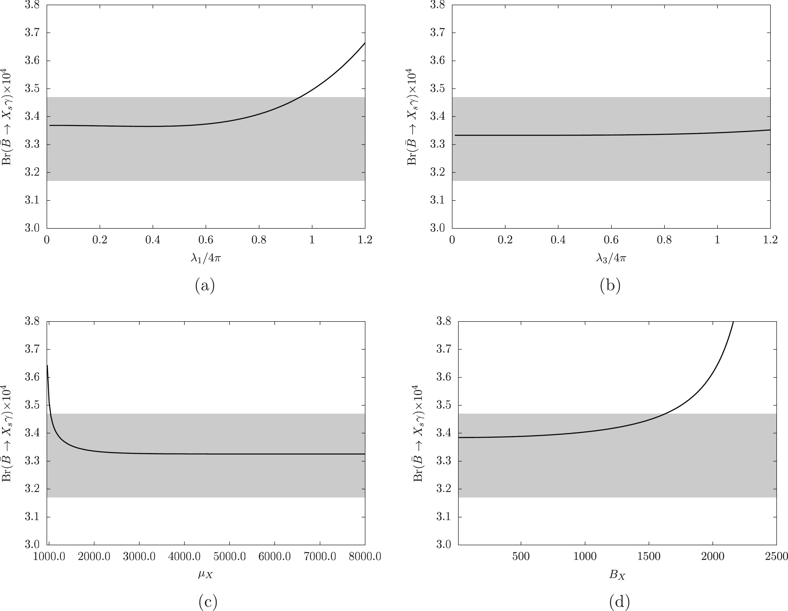
Figure 2. (color online)
$ Br(\bar{B}\to X_s\gamma) $ varying with parameters relevant to superfield$ X. $ In Fig. 2(a), one can find the branching ratio increases when
$ \lambda_1 $ increases. The experimental limitations are denoted by the gray area, and we have taken$ \lambda_3/(4\pi) = 0.07, \;\tan\beta = 10,\; \lambda_Q = 0.7,\; \lambda_U = 0.3,\; \lambda_D = 0.2, \; \mu = $ $ -600, \;\mu_B = m_{Z_B} = m_B = 1000,\; \mu_X = 1100, \;B_X = 400, \;v_{bt} = 6000.$ It can be seen in this figure that the branching ratio reachs the upper limits of experiments when$ \lambda_1/(4\pi) = 0.95 $ , giving the constraint$ \lambda_1/(4\pi)<0.95 $ .Similarly, we plot the branching ratio varying with
$ \lambda_3 $ in Fig. 2(b). By taking$ \lambda_1/(4\pi) = 0.07 $ , which satisfies the limitations obtained in Fig. 2(a), and$ \tan\beta = 5,\; \lambda_Q = 0.7, $ $ \lambda_U = 0.5,\; \lambda_D = 0.8, \;\mu = -800,\; \mu_B = \mu_X = 1100, \;m_{Z_B} = 1000, $ $ m_B = 500,\; B_X = 400, \; v_{bt} = 6000 $ , we find that the branching ratio rises very slowly when$ \lambda_3/(4\pi) $ runs from 0.01 to 1.5. The whole curve lies in the gray area, which means the branching ratio satisfies the experimental constraints under our assumptions.To investigate the variation of
$ Br(\bar{B}\to X_s\gamma) $ with$ \mu_X $ , we take$ \lambda_1/(4\pi) = 0.06,\; \lambda_3/(4\pi) = 0.08,\; \tan\beta = 5, \;\lambda_Q = $ $0.8, \; \lambda_U = 0.5, \; \lambda_D = 0.2, \;\mu = -600, \; \mu_B = 1000, \;B_X = 400, m_{z_B} = $ $1100, \; v_{bt} = 6000, \;m_B = 2500 $ . We find from Fig. 2(c) that the branching ratio decreases steeply with increasing$ \mu_X $ , and finally reaches the SM value. In Fig. 2(d), we plot the branching ratio varying with$ B_X $ , where we take$ \lambda_1/(4\pi) = 0.15,\; \lambda_3/(4\pi) = 0.08,\; \tan\;\beta=5, $ $ \lambda_Q=0.7, \; \lambda_U=0.2, $ $ \lambda_D = 0.3,\; \mu = -1000,\; \mu_B = 1100,\; \mu_X = 2500,\; m_{z_B} = 900,\; v_{bt} = $ $ 5500,\; m_B = 2000$ . With the upper limits of experimental results, we get the constraint$ B_X<1625 $ .In Fig. 3(a), we present the branching ratio varying with
$ \lambda_Q $ , which is the coupling in the superpotential term$ \lambda_{_Q}\hat{Q}_{_4}\hat{Q}_{_5}^c\hat{\Phi}_{_B} $ . With$ \lambda_1/(4\pi) = 0.08,\; \lambda_3/(4\pi) = 0.06, \tan\;\beta = 20, \; $ $ \lambda_U = 0.3,\; \lambda_D = 0.6,\; \mu = -800,\; \mu_B = 1000,\; \mu_X = 1200, B_X = $ $400, \; m_{z_B} = 1000,\; v_{bt} = 5000,\; m_B = 1500 $ , we find that the branching ratio decreases when$ \lambda_Q $ increases. To be consistent with the experimental data,$ \lambda_Q>0.62 $ . Another interesting parameter is$ v_{bt} $ , which is defined as$ v_{bt} = \sqrt{\bar{v}_B^2+v_B^2} $ , where$ v_B $ and$ \bar{v}_B $ are VEVs of$ \Phi_B $ and$ \varphi_B $ respectively. We plot the variation of the branching ratio with$ v_{bt} $ in Fig. 3(b) with$ \lambda_1/(4\pi) = \lambda_3/(4\pi) = 0.1,\; $ $ \tan\;\beta = 5,\; \lambda_Q = 0.7, \lambda_U = 0.2,\; \lambda_D = 0.7,\; \mu = -1000, \;\mu_B = 1100, $ $\mu_X = 1400,\; B_X = $ $ 400, \; m_{z_B} = 1000,\; m_B = 1500 $ . To satisfy the experimental constraints, we have$ v_{bt}>4200 $ .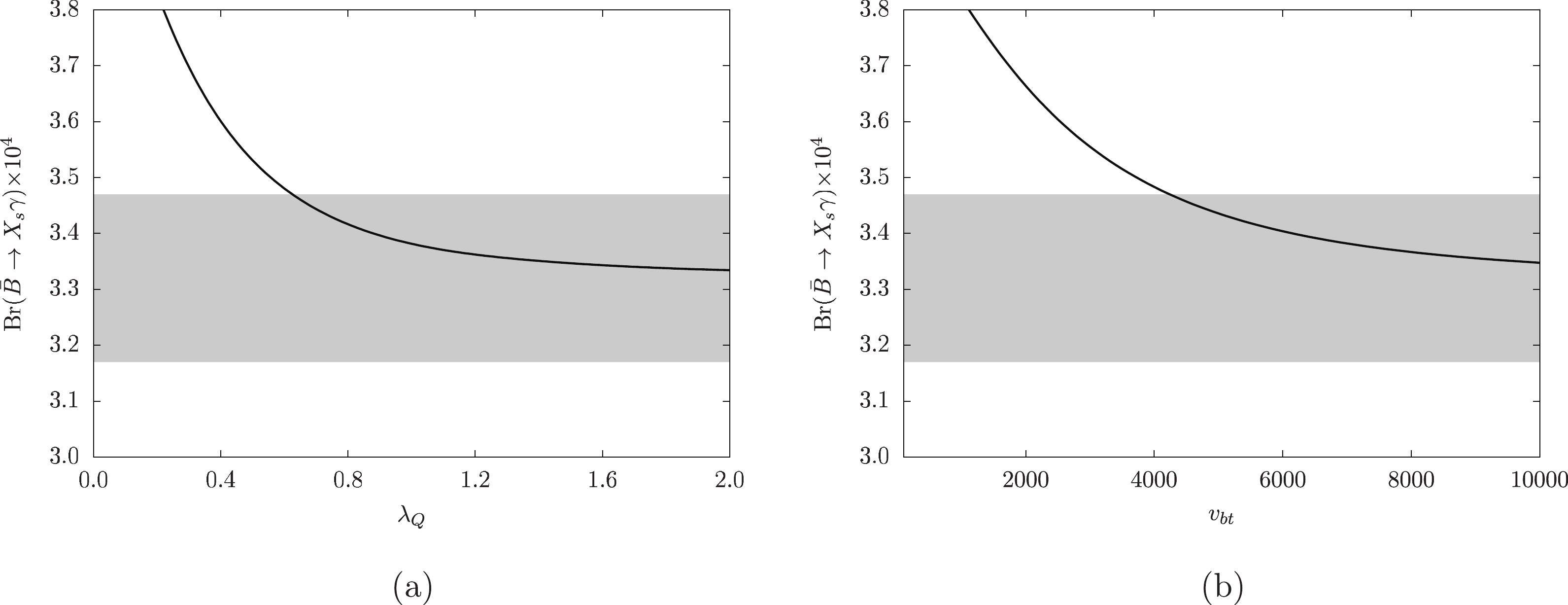
Figure 3. (color online)
$ Br(\bar{B}\to X_s\gamma) $ varying with$ \lambda_Q $ and$ v_{bt}. $ Additionally, we plot the direct CP-violation of
$ \bar{B}\to X_s\gamma $ and time-dependent CP-asymmetry of$ B\rightarrow K^*\gamma $ varying with$ \lambda_1,\; \lambda_3,\; \mu_X,\; B_X,\; \lambda_Q, \;\lambda_D $ and$ v_{bt} $ . Within the framework of the SM, we have$ -0.6 \%<A_{\rm CP}^{\rm SM}<+2.8 \% $ [33], and the average value of this observable is$ A_{\rm CP}^{\rm exp} = -0.009\pm 0.018 $ [34, 35]. Within some uncertainty, the theoretical value is consistent with the experimental result. Compared with the direct CP-violation of$ \bar{B}\to X_s\gamma $ , there is significant deviation between the SM prediction and the experimental result for$ S_{K^*\gamma} $ . The SM prediction for the time-dependent CP-asymmetry in$ B\rightarrow K^*\gamma $ at LO level is given as$ S_{K^*\gamma}^{\rm SM}\simeq (-2.3\pm1.6) \% $ [36], and the experimental result is$ S_{K^*\gamma}\simeq -0.15\pm 0.22 $ [34].To investigate
$ A^{\rm CP}_{\bar{B}\to X_s\gamma} $ and$ S_{K^*\gamma} $ numerically, some parameters are taken to be complex, and the areas within experimental boundaries are shown in gray in the presented figures. In Fig. 4, we plot the dependency of parameters relevant to superfield$ X $ . Under our assumptions of free parameters introduced in the BLMSSM, we find that$ A^{\rm CP}_{\bar{B}\to X_s\gamma} $ (solid line) is hardly affected by the change of$ \lambda_1,\; \lambda_3,\; \mu_X,\; B_X $ . Though corrections from one-loop level are almost zero, the numerical results are consistent with experimental data.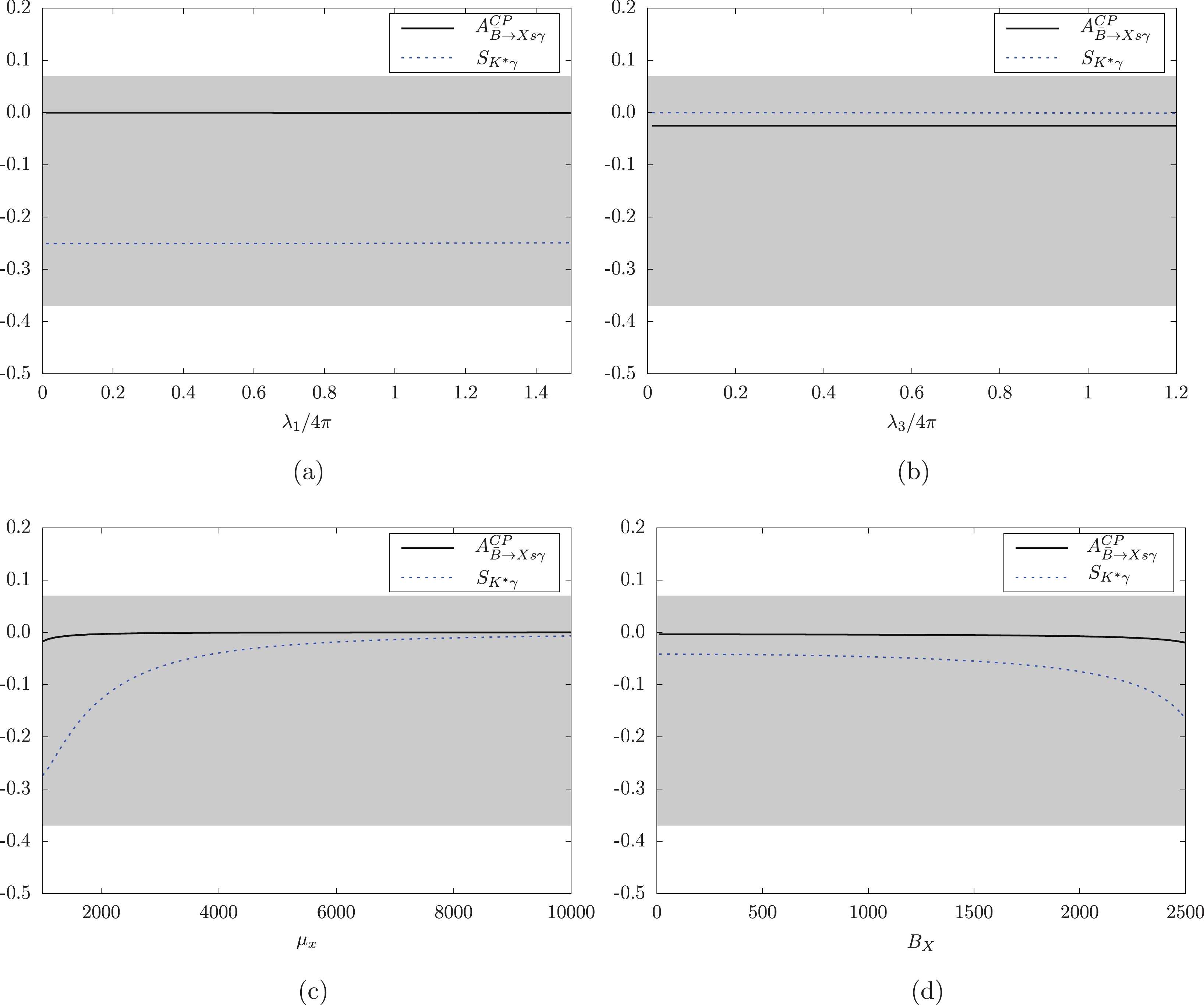
Figure 4. (color online)
$ A^{\rm CP}_{\bar{B}\rightarrow X_s\gamma} $ and$ S_{K^*\gamma} $ varying with parameters relevant to superfield$ X. $ As shown in Fig. 4(a), one-loop corrections to
$ S_{K^*\gamma} $ (dashed line) in the BLMSSM can reach$ -0.25 $ with appropriate inputs. By changing the free parameters, one finds$ S_{K^*\gamma} $ can be as small as zero in Fig. 4(b). In Fig. 4(c), it can be seen that$ S_{K^*\gamma} $ increases significantly with increasing$ \mu_X $ , and finally becomes stable around zero. The variation of$ S_{K^*\gamma} $ with$ B_X $ is given in Fig. 4(d). When$ B_X $ increases,$ S_{K^*\gamma} $ decreases. Within the range of parameters$ \lambda_1,\; \lambda_3,\; \mu_X $ and$ B_X $ , we find that$ S_{K^*\gamma} $ is consistent with experimental data.In Fig. 5, we take into account the parameters
$ \lambda_Q $ and$ \lambda_D $ . When$ \lambda_Q $ runs from 0.01 to 2.0, the time-dependent CP-asymmetry decreases from$ 0.02 $ to$ -0.22 $ , while for increasing$ \lambda_D $ ,$ S_{K^*\gamma} $ increases from$ -0.28 $ to$ -0.02 $ . Under our assumptions, we conclude that$ \lambda_Q $ and$ \lambda_D $ clearly affect$ S_{K^*\gamma} $ , and the numerical results for new physics corrections are consistent with experimental data. However, the direct CP-violation of$ \bar{B}\to X_s\gamma $ depends weakly on$ \lambda_Q $ and$ \lambda_D $ , and the one-loop contributions from the BLMSSM are very small.
Figure 5. (color online)
$ A^{\rm CP}_{\bar{B}\rightarrow X_s\gamma} $ and$ S_{K^*\gamma} $ varying with$ \lambda_Q $ and$ \lambda_D. $ The last Fig. 6 shows the variation of
$ S_{K^*\gamma} $ and$ A^{\rm CP}_{\bar{B}\to X_s\gamma} $ with$ v_{bt} $ . By taking$ \lambda_1/(4\pi) = 0.8,\; \lambda_3/(4\pi) =0.9, $ $ B_X = 400 $ and$ \lambda_Q = 0.4{\rm e}^{0.625\pi} $ , we find that$ S_{K^*\gamma} $ increases from$ -0.26 $ to$ -0.06 $ .$ A^{\rm CP}_{\bar{B}\to X_s\gamma} $ stays around zero within the range$ 100<v_{bt}<10000 $ .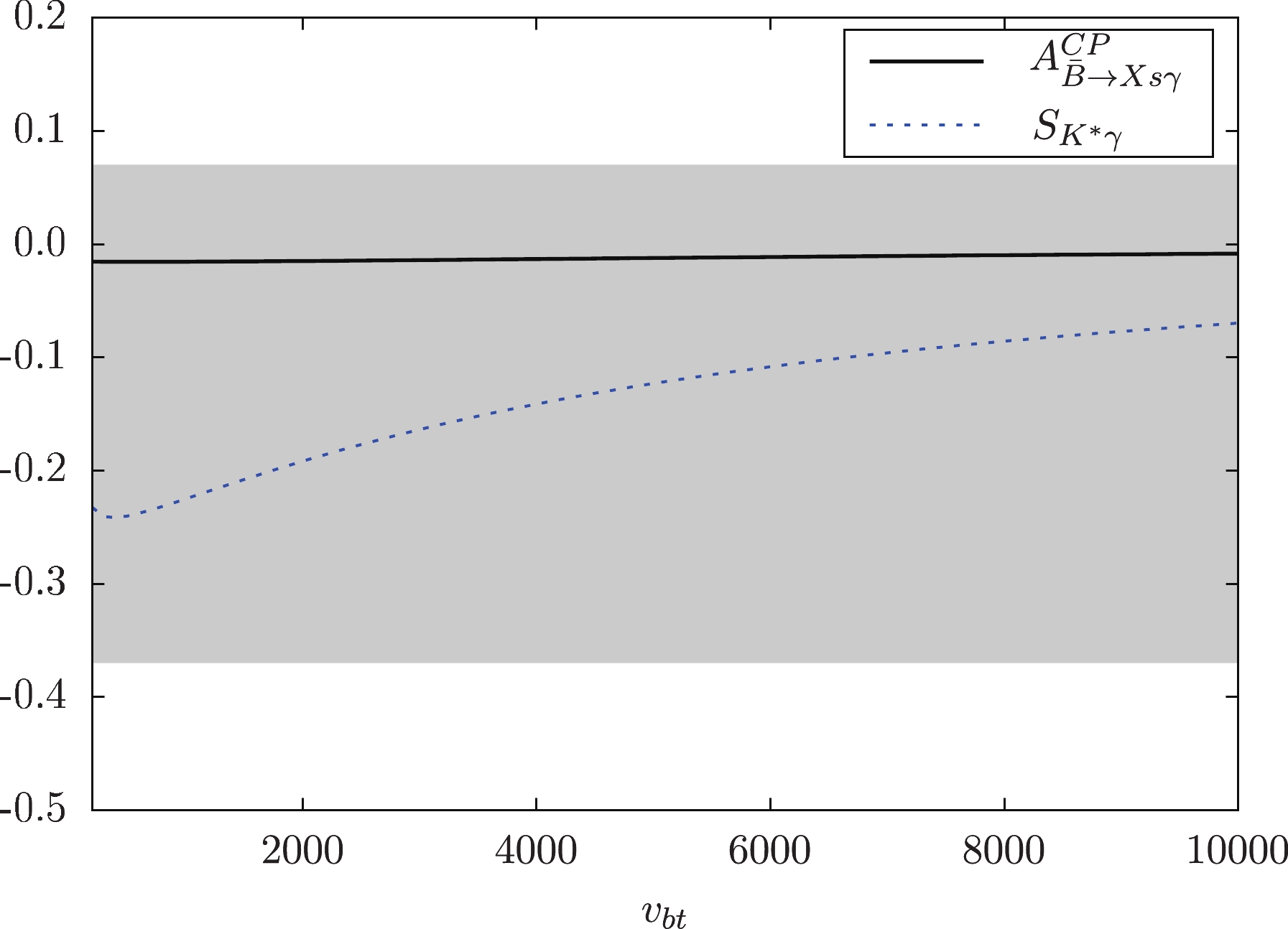
Figure 6. (color online)
$ A^{\rm CP}_{\bar{B}\rightarrow X_s\gamma} $ and$ S_{K^*\gamma} $ varying with$ v_{bt}. $ To analyze the dependence of Wilson coefficients and CP-asymmetry on the scale
$ \mu_b $ , the numerical results for$ C_{7,8}^{NP} $ ,$ \tilde{C}_{7,8}^{NP} $ ,$ A_{\rm CP} $ and$ S_{K^*\gamma} $ are given in Table 3. The input parameters are the same as in Fig. 5(b) with$ \lambda_D = 0.1 $ . It can be seen that the CP violation/asymmetry becomes more significant when$ \mu_b $ becomes larger. By printing the coefficients from different diagrams separately, one can find the dominant corrections come from Fig. 1(e), which contains the exotic squark charged -1/3 and superfield$ \tilde X $ .$ \mu_b $ 

$ |C_7^{NP}| $ 

$ |C_8^{NP}| $ 

$ |\tilde{C}_7^{NP}| $ 

$ |\tilde{C}_8^{NP}| $ 

$A_{\rm CP}$ 

$ S_{K^*\gamma} $ 

$ m_b/2=2.09 $ GeV

$ 0.078 $ 

$ 0.013 $ 

$ 0.053 $ 

$ 0.014 $ 

$ -0.019 $ 

$ -0.200 $ 

$ m_b=4.18 $ GeV

$ 0.100 $ 

$ 0.016 $ 

$ 0.067 $ 

$ 0.017 $ 

$ -0.025 $ 

$ -0.220 $ 

$ 2m_b=8.36 $ GeV

$ 0.118 $ 

$ 0.018 $ 

$ 0.078 $ 

$ 0.020 $ 

$ -0.028 $ 

$ -0.228 $ 

Table 3. Dependence of
$ C_{7,8}^{NP} $ ,$ \tilde{C}_{7,8}^{NP} $ ,$ A_{\rm CP} $ and$ S_{K^*\gamma} $ on typical scales. -
We have investigated the transition
$ b\to s\gamma $ , an interesting FCNC process, within the framework of the BLMSSM. With the effective Hamiltonian method, we have presented the Wilson coefficients extracted from amplitudes corresponding to the relevant one-loop diagrams. Based on the analytical expressions, constraints on parameters have been given in the numerical section, with the experimental data for the branching ratio of$ \bar{B}\to X_s\gamma $ . The direct CP-violation of$ \bar{B}\to X_s\gamma $ in the BLMSSM is very small, and depends weakly on the free parameters. However, the time-dependent CP-asymmetry$ S_{K^*\gamma} $ in$ B\rightarrow K^*\gamma $ varies significantly with$ \mu_X,\; B_X, $ $ \lambda_Q,\; \lambda_D $ and$ v_{bt} $ . The contributions from new physics can reach$ -0.28 $ under appropriate setup of the parameters.
$ { \bar{\mathit{\boldsymbol{B}}}\to{ {X_s \gamma }}}$
in BLMSSM
- Received Date: 2020-10-14
- Available Online: 2021-05-15
Abstract: Applying the effective Lagrangian method, we study the flavor changing neutral current process


 DownLoad: