


 Abstract
 HTML
HTML Reference
 Related
 PDF
PDF


-
Multiple experiments, including the type Ia supernova (SNIa) [1, 2], cosmic microwave background (CMB) anisotropies [3], large scale structure [4], and baryon acoustic oscillation (BAO) peaks [5], have consistently confirmed that our universe is experiencing a process of accelerating expansion. Theoretically, this acceleration needs a new driving component with repulsive gravity. In numerous theoretical paradigms, the exotic dark energy theory is the most studied. One essential parameter, i.e., the ratio of pressure to energy density, in the equation of state (EoS) w is designed to understand its nature. For example, the EoS of the famous cosmological constant model is
$ w = -1 $ . According to a recent analysis [6], this model fits well with the Planck and other astrophysical data. However, an evolving dark energy is also mildly favored by many other data, especially in the very recent extended BAO survey [7]. In this study, we investigated the quintessence [8-11], phantom [12], and tachyon [13-15] fields. They are all scalar fields that can achieve evolving dark energy. Concerning the quintessence field, it has a positive kinetic energy density with$ -1 \leqslant w \leqslant 1 $ . Regarding the phantom field, it has a negative kinetic energy density with$ w \leqslant -1 $ .However, numerous observations found that w was crossing
$ -1 $ . Unfortunately, neither the quintessence nor the phantom scalar field can fulfill this transition. To solve this issue, Feng et al. [16] proposed the quintom model, i.e., a combination of the quintessence field$ \phi_1 $ and phantom field$ \phi_2 $ in the Lagrangian. When the time derivative of the scalar field fulfills$ \dot{\phi}_1 > \dot{\phi}_2 $ , it leads to$ w \geqslant -1 $ ; conversely, for$ \dot{\phi}_1 < \dot{\phi}_2 $ , we have$ w \leqslant -1 $ . To promote the quintom model to be a single scalar field, Refs. [17-21] introduced higher derivative operators in the Lagrangian. They found that the models are consistent with the observations.Note that most of the potentials
$ V(\phi) $ were built by parametrization, either in the quintessence, phantom, or quintom models. Their common popular templates include the power-law potential, exponential potential, or trigonometric function potential. However, a parameterized$ V(\phi) $ template inevitably imposes a prior on the underlying property of cosmic dynamics. In our view, a straightforward and template-free study is advantageous to understand such cosmic dynamics.In this study, we focused on a prominent technique, i.e., the Gaussian processes (GP) method. Unlike the parametrization constraint, the GP method does not impose any artificial cosmological template. It is a purely statistical approach. In this process, a requirement is presented for each observational datum, that is, it must satisfy a Gaussian distribution. The data sets thus naturally satisfy a multivariate Gaussian distribution. In this process, we need a covariance function
$ k(z, \tilde{z}) $ to connect two variables between any two data points. Using the function$ k(z, \tilde{z}) $ , information of the variables contained in data can be extrapolated to other redshift that had not been observed. Finally, an involved goal function, such as the potential V in the scalar field, can be reconstructed via more data. Note that the determination of the function$ k(z, \tilde{z}) $ is the primary task in this Gaussian process. Given that this process is independent of any template for the goal function, it has been widely used in many fields, such as cosmology [22-31]. In a recent study of ours [32], we investigated the dark energy using this method. The EoS w analysis shows that observational data indicate a dynamical dark energy. However, the source of the dynamics is still unknown for us. Therefore, the nature of this reconstructed dark energy needs further understanding. In this study, we performed a relevant analysis via the scalar field. Our goal in the present study was to explore scalar fields that may constitute the dynamical source of dark energy. This test can update our understanding on the cosmic acceleration by presenting model-independent results. Following our aforementioned recent study, the data sets we used are still supernova and Hubble parameters, as well as perturbation data provided by the growth rate of structure. The dynamical models we considered are the quintessence, phantom, and tachyon scalar fields.This paper is organized as follows. In Section II, we introduce the scalar field and GP approach. In Section III, we introduce the relevant data we used. We present the reconstruction results in Section IV. Finally, in Section V, conclusions and discussions are presented.
-
In this section, we give an introduction about the scalar field and GP approach.
-
For a Friedmann-Robertson-Walker universe with flat spatial, we assume it has only dark matter and a scalar field. The Friedman equations of this universe are
$ \begin{aligned}[b] H^2 &= \frac{8\pi G}{3} (\rho_m + \rho_{\phi} ), \\ \frac{\ddot{a}}{a} &= -\frac{4\pi G}{3} (\rho_m + \rho_{\phi} + 3 p_{\phi}) , \end{aligned} $

(1) where the Hubble expansion rate
$ H = \dot{a}/a $ is a function of the scalar factor$ a(t) $ , and the dot denotes derivative with respect to cosmic time t. The parameters$ \rho_{\phi} $ and$ p_{\phi} $ are energy density and pressure of the scalar field, respectively. Concerning the dark matter, we assume that its energy density yields$ \rho_m = \rho_{m0} (1+z)^3 $ , where$ \rho_{m0} $ is its current energy density. Generally, we introduce the matter energy density parameter$ \Omega_{m0} = \rho_{m0}/\rho_{c0} $ , with critical density$ \rho_{c0} = 3H_0^2/ (8 \pi G) $ , where$ H_0 $ is the Hubble constant. Regarding the scalar field, we considered three scenarios in the present study, namely, the quintessence, phantom, and tachyon scalar fields.Concerning the quintessence scalar field, its energy density and pressure are defined as
$ \begin{aligned}[b] \rho_{\phi} &= \frac{1}{2}\dot{\phi}^2 + V(\phi) , \\ p_{\phi} &= \frac{1}{2}\dot{\phi}^2 - V(\phi) . \end{aligned} $

(2) The potential
$ V(\phi) $ is usually parameterized as a function of the scalar field$ \phi $ . To date, many models were proposed (see Ref. [33] for a short review), such as the power-law potential$ V(\phi) \propto \phi^{p} $ , exponential potential$ V(\phi) \propto e^{-{\rm{\lambda }} \phi} $ , inverse power-law potential$ V(\phi) \propto \phi^{-p} $ , inverse exponential potential$ V(\phi) \propto e^{{\rm{\lambda }}/ \phi} $ , double exponential potential$ V(\phi) \propto V_1 e^{-{\rm{\lambda }}_1 \phi} + V_2 e^{-{\rm{\lambda }}_2 \phi} $ , and Hilltop potential$ V(\phi) \propto \cos(\phi) $ . Other complex models can also be found in Ref. [34], such as$ e^{{\rm{\lambda }} \phi^2}/\phi^{\alpha} $ ,$ (\cosh {\rm{\lambda }} \phi -1)^p $ ,$ \sinh ^{-\alpha} ({\rm{\lambda }} \phi) $ , and$ [(\phi - B)^{\alpha} + A] e^{-{\rm{\lambda }} \phi} $ . As a result of confronting these models with the observational data [35-39], the authors found that some models cannot be discriminated from each other. It was also found that some models are not disfavored by the observational data, such as the inverse power-law potential and inverse exponential potential, and others have intrinsic limitations. In this study, we strongly aimed at determining suitable models for describing the dark energy. Thus, our objective was to solve the quintessence scalar field. By introducing the definitions expressed by Eq. (2) into Friedman equations in Eq. (1), we can solve the quintessence field. Its potential is$ \begin{aligned}[b] \frac{8\pi G}{3H_{0}^2} \dot{\phi}^{2} &= \frac{1}{3}(1+z) E^{2 \prime} - \Omega_{m0} (1+z)^3 , \\ \frac{8\pi G}{3H_{0}^2} V &= E^2 - \frac{1}{6}(1+z) E^{2 \prime} - \frac{1}{2}\Omega_{m0} (1+z)^3 , \end{aligned}$

(3) where the prime denotes derivative with respect to redshift z, and
$ E(z) = H(z)/H_0 $ is the dimensionless Hubble parameter. We found, on the one hand, that both the derivative of scalar field$ \dot{\phi}^{2} $ and potential V are in units of$\dfrac{8\pi G}{3H_{0}^2}$ . On the other hand, note that the function$ \dot{\phi}^{2} $ may be negative when the former term is less than the latter term. If this is the case, it would change into the other model, i.e., the phantom scalar field.Concerning the phantom scalar field, its energy density and pressure are
$ \begin{aligned}[b] \rho_{\phi} &= -\frac{1}{2}\dot{\phi}^2 + V(\phi) , \\ p_{\phi} &= -\frac{1}{2}\dot{\phi}^2 - V(\phi) . \end{aligned} $

(4) Performing a similar calculation, we can obtain the phantom field and potential
$ \begin{aligned}[b] \frac{8\pi G}{3H_{0}^2} \dot{\phi}^{2} &= \Omega_{m0} (1+z)^3 - \frac{1}{3}(1+z) E^{2 \prime} , \\ \frac{8\pi G}{3H_{0}^2} V & = E^2 - \frac{1}{6}(1+z) E^{2 \prime} - \frac{1}{2}\Omega_{m0} (1+z)^3 . \end{aligned} $

(5) Evidently, the function
$ \dot{\phi}^{2} $ in Eq. (5) is opposite to$ \dot{\phi}^{2} $ in Eq. (3). Therefore, the quintessence and phantom fields cannot exist simultaneously. Similar to above quintessence scalar field, the cosmologist also modelled many phantom potentials. Caldwell et al. [40] studied this scalar field, and found that$ w<-1 $ would cause a significant rip of the universe. Another study [41] considered five models, and showed that they fit well with the observational data, with no special position being occupied. To solve the problem of w crossing$ -1 $ in the near past from$ w > -1 $ to$ w < -1 $ , Feng et al. [16] proposed a quintom model with a double exponential potential in the Lagrangian by combining the quintessence and phantom fields$ \begin{aligned}[b] {\cal{L}} = &\frac{1}{2} \partial_{\mu} \phi_1 \partial^{\mu} \phi_1 - \frac{1}{2} \partial_{\mu} \phi_2 \partial^{\mu} \phi_2 \\ &- V_0 \left[\exp\left(-\frac{{\rm{\lambda }}}{m_p} \phi_1\right) + \exp\left(-\frac{{\rm{\lambda }}}{m_p} \phi_2\right) \right] , \end{aligned}$

(6) where
$ \phi_1 $ and$ \phi_2 $ denote the quintessence and phantom fields, respectively. Note that this is different from the quintessence or phantom fields. It presents more complicated dynamics. The authors found that this model also satisfies the observations. The parameters were set as$ V_0 = 8.38 \times 10^{-126} m_p^4 $ and$ {\rm{\lambda }} = 20 $ . This model can realize the transition of w from$ w > -1 $ to$ w < -1 $ .Concerning the tachyon scalar field, it is a different scalar field with respect to the two aforementioned scenarios. Its energy density and pressure are
$ \begin{aligned}[b] \rho_{\phi} & = \frac{V(\phi)}{\sqrt{1-\dot{\phi}^2}} , \\ p_{\phi} & = -V(\phi) \sqrt{1-\dot{\phi}^2} . \end{aligned} $

(7) In combination with the Friedman equations, i.e., Eq. (1), the tachyon field and potential can be solved as
$ \begin{aligned}[b] \dot{\phi}^{2} &= \frac{(1+z) E^{2 \prime} - 3\Omega_{m0} (1+z)^3}{ 3E^2 - 3\Omega_{m0} (1+z)^3} , \\ \frac{8\pi G}{3H_{0}^2} V &= \sqrt{E^2-\frac{1+z}{3} E^{2 \prime}} \sqrt{E^2 - \Omega_{m0} (1+z)^3} . \end{aligned} $

(8) Several points must be highlighted about this solution. First, the term
$ 1-\dot{\phi}^2 $ in Eq. (7) must be positive. Second, we found that the solutions$ \dot{\phi}^{2} $ and V in Eq. (8) are notably different from the ones in the two scenarios previously described. Regarding the function$ \dot{\phi}^{2} $ , it is immune from the nuisance parameter$\dfrac{8\pi G}{3H_{0}^2}$ . Concerning the potential V, it should be non-negative in the square root of Eq. (8). Evidently, any negative values in Eq. (8) can lead to failure of the tachyon field. In cosmology, several tachyon models were studied. In Ref. [42], the authors numerically investigated tachyon models with a range of potentials. Compared with the canonical quintessence models, they exhibit similar phenomenology. In Ref. [43], the authors also studied some models, and found that some of them are not strongly disfavoured by observations. For a single tachyon field with an inverse square potential, Guo et al. [44] found that the universe could accelerate only at nearly Planck energy densities. However, the acceleration can also be obtained for multiple tachyon fields at lower-Planck energy densities.To obtain the potential
$ V(\phi) $ , we must solve the field$ \phi $ from the function$ \dot{\phi}^{2} $ . Using the relation${\rm d}t = -\dfrac{1}{(1+z)H} {\rm d}z$ , we can transfer the derivative of the scalar field$ \dot{\phi}^{2} $ over time t to redshift z, namely,$ \left( \frac{{\rm d}\phi}{{\rm d}z} \right)^2 = \frac{\dot{\phi}^{2}}{(1+z)^2 H^2} . $

(9) Here, we must be careful with the units of the function
$\left( \dfrac{{\rm d}\phi}{{\rm d}z} \right)^2$ in different scenarios. In our calculations, we reduced it to a dimensionless quantity. To obtain such a dimensionless quantity, the function$ \dot{\phi}^2 $ in the quintessence and phantom fields, and the potential$ V(z) $ in the three fields are in units of$\dfrac{8\pi G}{3H_{0}^2}$ . The function$\dfrac{{\rm d}\phi}{{\rm d}z}$ is in units of$ H_0 $ . Theoretically, the function$\dfrac{{\rm d}\phi}{{\rm d}z}$ can take two signs. In this study, we considered positive values. Finally, the scalar field can be obtained by$ \phi = \int \frac{{\rm d}\phi}{{\rm d}z} {\rm d}z . $

(10) In our calculations, we set an initial value
$ \phi_0 = 0 $ . Therefore, the scalar field$ \phi (z) $ can be obtained over a function of redshift z. After performing the preparations above described, the dimensionless potential$ V (z) $ and scalar field$ \phi (z) $ can be simultaneously reconstructed. Thus, the potential$ V(\phi) $ can be modelled as a function of the scalar field via a model-independent approach. -
The data we used in this study are background data from supernova and Hubble parameters and perturbation data from redshift-space distortions (RSD).
Concerning the background data, the theoretical distance modulus of supernova in the Friedmann-Robertson-Walker universe is
$ \mu_{\rm{th}} (z) = 5 {\rm{log}}_{10}d_L(z)+25, $

(11) with luminosity distance function
$ d_L(z) = \frac{c}{H_0} (1+z) \int^z_0 \frac{ {\rm{d}} \tilde{z}}{E(\tilde{z})} . $

(12) By introducing a dimensionless comoving luminosity distance
$ D(z) \equiv \frac{H_0}{c} \frac{d_L (z)}{1+z} , $

(13) we can obtain the relation between the Hubble parameter and distance
$ D(z) $ via Eqs. (13) and (12),$ E (z) = \frac{ 1}{D'} . $

(14) Therefore, the Hubble parameter data can be used as the derivative of the distance function
$ D(z) $ .Concerning the perturbation data, we considered a background universe filled with dark matter and scalar field as the unclustered dark energy. Regarding the dark matter, its density contrast is defined as
$ \delta(z) \equiv \dfrac{\delta \rho_m}{\rho_m} (z) $ . At scales much smaller than the Hubble radius, the evolution of the density contrast must obey a second order differential equation,$ \ddot{\delta} + 2H \dot{\delta} -4\pi G \rho_m \delta = 0 , $

(15) where
$ \rho_m $ is the background matter energy density, and$ \delta \rho_m $ represents its first-order perturbation. This is an equation describing matter growth under the assumption of homogeneity and isotropy with zero dark energy perturbations. The density contrast is in the linear regime, i.e.,$ \delta \ll 1 $ . If the dark energy is clustered, the perturbation would influence the evolution of the matter density contrast [45-48]. Thus, the anisotropic stress of the dark energy fluid proves to be an important discriminator between modified gravity and dark energy models. The authors also concluded that anisotropic stress affects the weak lensing and galaxy power spectrum.According to the relation between scale factor and redshift, we can transfer the derivative of the density contrast
$ \delta $ over cosmic time t into derivative over redshift z. Thus, the Hubble parameter in Eq. (15) can be expressed as [49, 50]$ E^2(z) = 3 \Omega_{m0} \frac{(1+z)^2}{\delta '(z) ^2 } \int_z^{\infty} \frac{\delta}{1+z} (-\delta ') {\rm d} z . $

(16) We found that the Hubble parameter
$ E^2(z) $ tends to zero when the redshift in the integral implies$ z \rightarrow \infty $ . When the redshift$ z = 0 $ , we have the initial condition$ 1 = \frac{3 \Omega_{m0}}{\delta '(z = 0) ^2} \int_0^{\infty} \frac{\delta}{1+z} (-\delta ') {\rm d} z . $

(17) Using this initial condition, we rewrite the Hubble parameter in Eq. (16) as
$ E^2(z) = (1+z)^2 \dfrac{\delta '(z = 0) ^2}{\delta '(z) ^2 } \left[ 1 - \frac{\displaystyle\int_0^{z} \dfrac{\delta}{1+z} (-\delta ') {\rm d} z}{\displaystyle\int_0^{\infty} \dfrac{\delta}{1+z} (-\delta ') {\rm d} z} \right] . $

(18) Observationally, the perturbation
$ \delta(z) $ cannot be directly measured by current cosmological surveys, but can be provided by a related observation. It is the growth rate measurement$ f\sigma_8 $ from RSD. Here, the function f denotes the growth rate, which is defined by the derivative of the logarithm of perturbation$ \delta $ with respect to the logarithm of the cosmic scale$ f \equiv \frac{{\rm d} \, {\rm{ln}} \delta}{{\rm d} \, {\rm{ln}} a} = -(1+z) \frac{{\rm d} \, {\rm{ln}} \delta}{{\rm d} \, z} = -(1+z) \frac{\delta '}{\delta} . $

(19) The function
$ \sigma_8 (z) = \sigma_8 (z = 0) \frac{\delta (z)}{\delta (z = 0)} $

(20) is the linear theory root-mean-square mass fluctuation within a sphere of radius
$ 8h^{-1} $ Mpc. According to the above two definitions, their combination is written as$ f \sigma_8 = -\frac{\sigma_8 (z = 0)}{\delta (z = 0)} (1+z) \delta ' , $

(21) which is called the growth rate of structure. Therefore, we can obtain
$ \delta ' = - \frac{\delta (z = 0)}{\sigma_8 (z = 0)} \frac{f \sigma_8}{1+z} . $

(22) Evidently, we can reconstruct the derivative
$ \delta ' $ of the perturbation via the observational RSD data$ f \sigma_8 $ . Taking an integral to the two sides of Eq. (22) over redshift, we have$ \delta = \delta (z = 0) - \frac{\delta (z = 0)}{\sigma_8 (z = 0)} \int_0^{z} \frac{f \sigma_8}{1+z} {\rm d}z . $

(23) For the constant
$ \delta (z = 0) $ , the normalization value is usually considered, i.e.,$ \delta (z = 0) = 1 $ [32]. Concerning the other constant, we set it as$ \sigma_8 (z = 0) = 0.8159 $ [6].Generally, to obtain the goal function
$ g(z) $ , the parametrization constraint usually restricts the application of a prior template on it. Departing from this method, the GP technique is model-independent, that is, it does not rely on any particular dynamical parametrization. It only needs a probability prior on the goal function$ g(z) $ . In this study, we assumed that each observational distance D obeys a Gaussian distribution with a particular mean and variance. Consequently, the posterior distribution of all observed distances D would obey a joint Gaussian distribution. Note in this process that the covariance function$ k(z, \tilde{z}) $ is a key ingredient. It correlates the distance$ D(z) $ at different points z and$ \tilde{z} $ . Commonly, we have several types on the covariance function$ k(z, \tilde{z}) $ . Most of them are associated with two hyperparameters,$ \sigma_f $ and$ \ell $ , which can be determined by observational data via a marginal likelihood. By training the covariance function, we can extend the distance$ D(z) $ to more redshift points. If we want to reconstruct the goal function$ g(z) $ , such as w for the dark energy, we must use the relation between the and distance D. Given that this method is model-independent, it has been widely applied to reconstruct the dark energy EoS [22], or to test the concordance model [23, 24].In the GP method, many types of covariance function
$ k(z, \tilde{z}) $ are available. In the present study, we adopted the most commonly used form, i.e., squared exponential,$ k(z, \tilde{z}) = \sigma_f^2 \exp \left[\frac{-|z-\tilde{z}|^2}{2 \ell^2} \right] . $

(24) With this covariance function, the scalar field can be reconstructed. We modified the package GaPP, which is publicly available in Ref. [22]. We also recommend this reference because many more details on the GP method can be found.
In the above framework, we introduced the background evolution of the scalar field. For the sake of a comprehensive study, the perturbation of the scalar field was extensively researched. In the conformal Newtonian gauge, the perturbed metric is
$ {\rm d}s^2 = a^2(\tau) [(1 + 2\Psi){\rm d}\tau ^2 -(1 -2\Phi){\rm d}x^i {\rm d}x_i] . $

(25) Concerning the quintom field, the perturbation equation was obtained as follows [51]
$\begin{aligned}[b] \dot{\delta}_i =& -(1 + w_i) (\theta_i - 3\dot{\Phi}) - 3{\cal{H}}(1-w_i) \delta_i \\ &- 3{\cal{H}} \frac{\dot{w}_i + 3{\cal{H}}(1-w_i^2)}{k^2} \theta_i , \end{aligned}$

(26) $ \dot{\theta}_i = 2{\cal{H}} \theta_i + \frac{k^2}{1 + w_i} \delta_i + k^2 \Psi , $

(27) where the subscript i in each case denotes the quintessence and phantom fields, respectively. The function
$ \theta_i $ is defined as$ \theta_i = (k^2 / \dot{\phi}_i) \delta \phi_i $ . We can refer to studies by Gong-Bo Zhao et al. [52] and Yi-Fu Cai et al. [53]. In Ref. [52], the authors considered a potential$ V(\phi) = \dfrac{1}{2} m_i^2 \phi_i^2 $ . The authors studied the radiation-dominated period and matter-dominated era, respectively. Using the specific scalar factor$ a = A \tau $ and Hubble parameter$ {\cal{H}} = 1/\tau $ , they obtained the solution of the scalar fields$ \phi_1 $ and$ \phi_2 $ . However, note that the potential V, scalar factor a, and Hubble parameter$ {\cal{H}} $ in this study are model-dependent. It is difficult to reconstruct the potential V and scalar field$ \phi $ without artificial perturbations$ \Psi $ and$ \Phi $ . However, note that a model-independent reconstruction of$ f(T) $ gravity was performed via Gaussian processes [54, 55]. In future work, we would also like to perform a further analysis on the quintom scalar field under reasonable assumptions and approximations. -
In this section, we introduce the related observational data.
Regarding supernova data, they were extracted from the joint light-curve analysis (JLA) datasets issued by the SDSS-II and SNLS surveys [56]. The redshifts of these JLA samples have a wide span of
$ 0.01 <z <1.3 $ . These samples contain a total of 740 SNIa data points. They include three-season data from SDSS-II ($ 0.05 < z <0.4 $ ), three-year data from SNLS ($ 0.2 < z <1 $ ), HST data ($ 0.8 < z <1.4 $ ), and several low-redshift samples ($ z <0.1 $ ). For these supernova samples, the data are usually presented in tabular form, including distance modulus and errors. For each SNIa, its distance modulus is given by$ \mu_{\rm{SN}} = m^{\star}_{B}+\alpha\cdot X_{1}-\beta\cdot {\cal{C}}-M_{B}\;, $

(28) where
$ m^{\star}_{B} $ is the observed peak magnitude in rest frame B band, the parameter$ X_{1} $ is the time stretching of light-curve, and the parameter$ {\cal{C}} $ describes the supernova color at maximum brightness. The last parameter$ M_{B} $ is the absolute B-band magnitude, which is assumed to be related to the host stellar mass ($ M_{\rm{stellar}} $ ) by a simple step function [56]:$ M_{B} = \left\lbrace \begin{array}{l} M^{1}_{B}\; \; \; \; \; \; \; \; \; \; \; \; \; \; \; {\rm{for}}\; \; \; M_{\rm{stellar}}<10^{10}M_{\odot},\\ M^{1}_{B}+\Delta_{M}\; \; \; \; \; {\rm{otherwise}}. \\ \end{array} \right. $

(29) Note that
$ \alpha $ ,$ \beta $ ,$ M^{1}_{B} $ , and$ \Delta_{M} $ are nuisance parameters in our calculation. They must be determined simultaneously with other cosmological parameters.To determine the nuisance parameters, the observed data are usually fit in a
$ \Lambda $ CDM cosmology [27, 56]. In the calculation, the full covariance matrix Cov of the JLA sample is defined as$ {\bf{Cov}} = {\bf{D}}_{\rm{stat}}+{\bf{C}}_{\rm{stat}}+{\bf{C}}_{\rm{sys}}\;. $

(30) Here, the matrix
$ {\bf{D}}_{\rm{stat}} $ is the diagonal part of the statistical uncertainty. It can be expressed as$ \begin{aligned}[b] ({\bf{D}}_{\rm{stat}})_{ii} =& \sigma^{2}_{m_{B},i}+\alpha^{2}\sigma^{2}_{X_{1},i}+\beta^{2}\sigma^{2}_{{\cal{C}},i} +2\alpha C_{m_{B}\,X_{1},\,i}-2\beta C_{m_{B}\,{\cal{C}},\,i}\\ &-2\alpha\beta C_{X_{1}\,{\cal{C}},\,i}+\sigma^{2}_{\rm{lens}}+\left(\frac{5\sigma_{z,i}}{z_{i}\ln 10}\right)^{2}+\sigma^{2}_{\rm{coh}}\; . \end{aligned} $

(31) In the first line,
$ \sigma_{{m_{B}},i} $ describes the standard errors of the peak magnitude;$ \sigma_{X_{1},i} $ , and$ \sigma_{{{\cal{C}}},i} $ are standard errors of the above light-curve parameters$ X_1 $ and$ {\cal{C}} $ , respectively. In the second line, the terms$ C_{m_{B}\,X_{1},\,i},\;C_{m_{B}\,{\cal{C}},\,i} $ , and$ C_{X_{1}\,{\cal{C}},\,i} $ respectively denote the covariances among the observed quantities$ m_{B},\;X_{1},\;{\cal{C}} $ for the i-th SN. In the last line, the term$ \sigma^{2}_{\rm{lens}} $ denotes the variation of magnitudes caused by gravitational lensing. The second term denotes the uncertainty in cosmological redshift produced by peculiar velocities. The term$ \sigma^{2}_{\rm{coh}} $ is the intrinsic variation in SN magnitude. In Eq. (30),$ {\bf{C}}_{\rm{stat}} $ and$ {\bf{C}}_{\rm{sys}} $ respectively denote the statistical matrices and systematic covariance matrices. They can be given by$ {\bf{C}}_{\rm{stat}}+{\bf{C}}_{\rm{sys}} = V_{0}+\alpha^{2}V_{a}+\beta^{2}V_{b} +2\alpha V_{0a}-2\beta V_{0b}-2\alpha \beta V_{ab}\;, $

(32) where
$ V_{0} $ ,$ V_{a} $ ,$ V_{b} $ ,$ V_{0a} $ ,$ V_{0b} $ , and$ V_{ab} $ are related matrices (refer to Ref. [56]). Because of the degeneracy between the Hubble constant$ H_{0} $ and the parameter$ M_{B} $ in constructing the Hubble diagram, we considered their effects on the scalar field reconstruction in the present study. According to the results in Ref. [27], we respectively ha-ve$ (\alpha,\beta,M^{1}_{B},\Delta_{M}) = (0.14\pm0.01,3.10\pm0.09, -19.08\pm 0.02, -0.07 \pm 0.03) $ in the prior of$ H_{0} = 69.6 \pm 0.7 $ km$ {\rm{s}}^{-1} $ $ {\rm{Mpc}}^{-1} $ , and$ (\alpha,\beta,M^{1}_{B},\Delta_{M}) = (0.14\pm0.01,3.11\pm0.09,-19.01\pm0.02, -0.07\pm0.03) $ in the Gaussian prior of$ H_{0} = 73.24 \pm 1.74 $ km$ {\rm{s}}^{-1} $ $ {\rm{Mpc}}^{-1} $ . In addition, we must take into account the theoretical initial conditions$ D(z = 0) = 0 $ and$ D'(z = 0) = 1 $ in the related calculation.Regarding
$ H(z) $ data, direct products cannot be obtained from a tailored telescope. However, two approaches are available to acquire them. The first one is called cosmic chronometer, which is based on the calculation of differential ages of galaxies [57-59]. The second approach is derived from the BAO peaks. To be specific, we can deduce it from the galaxy power spectrum [60, 61] or from the Ly$ \alpha $ forest of QSOs [62]. For the latter method, an underlying cosmology increases its model-dependence in the calculation of the sound horizon. In this study, we used the 30 cosmic chronometer data points. We compiled them in a recent work of ours [25]. Considering the uncertainty of the Hubble constant, the uncertainty of$ E(z) $ can be determined as$ \sigma_E^2 = \frac{\sigma_H^2}{H_0^2} + \frac{H^2}{H_0^4} \sigma_{H_0}^2 . $

(33) Using the prior of
$ H_0 $ , namely$ H_0 = 73.24 \pm 1.74 $ km s$ ^{-1} $ Mpc$ ^{-1} $ with 2.4% uncertainty [63] and$ H_0 = 69.6 \pm 0.7 $ km s$ ^{-1} $ Mpc$ ^{-1} $ from the 1% determination [64], uncertainty of the dimensionless Hubble parameter can be calculated. Departing from most of previous studies, we used them through combination with supernova data, rather than using$ H(z) $ data alone. That is, the Hubble parameter was used as a derivative of the distance D,$ D' = \dfrac{1}{E(z)}. $ Meanwhile, we must consider$ E(z = 0) = 1 $ as an initial condition in our calculation.Concerning the RSD data, they can be obtained from the galaxy distribution observation. In particular, they are generated from an effect. In galaxy distribution measurements, the observed distance of a galaxy is different from its true distance in redshift space. This is because velocities in the overdensities deviate from the cosmic smooth Hubble flow expansion. It is known that the cosmic structure growth is correlated with the anisotropy in the clustering of galaxies. According to General Relativity, an anisotropy can be produced. Moreover, a smaller deviation from this theory indicates a smaller anisotropic distortion. In virtue of the above distinct superiority, RSD data are very promising in distinguishing the cosmological models. Because of its sensibility, a similar background evolution has a very distinct growth of structure in different cosmological models. To date, many studies used RSD data to study cosmology. In the present study, the most recent RSD data from 6dFGS, 6dFGRS, SDSS MGS, SDSS LRG, GAMA, BOSS DR12, WiggleZ, VIPERS, FastSound, and BOSS DR14 redshift surveys were utilized. Because some data are cosmology-dependent and the covariance for different datasets is unknown [65], we used the compilation from Planck Collaboration [66]. For these data, the BOSS DR12 and WiggleZ present a full covariance matrix, including systematic errors.
-
Note that the determination of the scalar fields and potentials introducted in Section II is dependent on the matter density parameter
$ \Omega_{m0} $ , Hubble parameter$ E(z) $ , and its derivative$ E'(z) $ . Concerning the matter density parameter, we considered a moderate estimation, i.e.,$ \Omega_{m0} = 0.279 \pm 0.025 $ [67]. Concerning the function$ V(\phi) $ , actively researched in previous studies, many models were proposed in the past few decades, as mentioned above. In this study, we first reconstructed the scalar field$ \phi (z) $ over the redshift z and potential$ V(z) $ using the GP method; then, we tried to fit the function$ V(\phi) $ using their mean values. Owing to the model-independence of the GP method, we consider that it can provide a more scientific test on the scalar field. Therefore, we expect a better understanding about the dynamics of dark energy. -
To test the effect of the Hubble constant on the corresponding reconstructions, we distribute the results in two subsections.
$ 1.\;\; H_0=73.24 \pm 1.74 \; {\rm{km}} \;{\rm s} ^{-1} {\rm {Mpc}} ^{-1} $

In Figs. 1 and 2, we plot the derivative of scalar field,
$ \dot{\phi}^2 $ , and the potential V in the quintessence and tachyon fields with$ H_0 = 73.24 \pm 1.74 $ km s$ ^{-1} $ Mpc$ ^{-1} $ . Theoretically, the function$ \dot{\phi}^2 $ should be$ \dot{\phi}^2 \geqslant 0 $ . Indeed, the plots show that$ \dot{\phi}^2 $ in these two fields are positive within 68% confidence level at low redshift. However, it turns to negative at high redshift. Moreover, it is difficult to determine the sign of this function within 95% confidence level. Concerning the potential V in these two fields, it increases softly first and then sharply at redshift$ z \sim 1.0 $ in both cases. The initial value is$ V_0 = 0.70 $ . In Ref. [42], the authors found that the tachyon models considered in their study presented phenomenology similar to that of the canonical quintessence models. Comparing the reconstructions in these two plots, they are really similar. Let us now return to the function$ \dot{\phi}^2 $ . The vacillating$ \dot{\phi}^2 $ indicates that the single quintessence field, phantom field, or tachyon field are all difficult to be favored by the data. Therefore, we cannot depict the function$ V(\phi) $ using a single field. However, because the function$ \dot{\phi}^2 $ in the quintessence field and the phantom field are opposite, we can also conclude that it keeps switching between the two fields. Consequently, the quintom field proposed by Feng et al. [16] may be a better building on the scalar field. Next, we treated the GP reconstruction in Fig. 1 as a quintom field, i.e., as a combination of quintessence and phantom fields. According to their mean values, we found that the function$ \dot{\phi}^2 $ changes from$ \dot{\phi}^2 < 0 $ to$ \dot{\phi}^2 > 0 $ , which indicates that the scalar field changes from the phantom field to the quintessence field with the cosmic evolution. Solving the Eq. (10), we can acquire the scalar field$ \phi (z) $ over the redshift z, as shown in Fig. 3. We found that the scalar field$ \phi (z) $ increases with the increasing redshift. Using the mean values of$ \phi (z) $ and$ V (z) $ , we eventually obtained the potential$ V (\phi) $ as a function of the field$ \phi $ . The potential is also an increasing function. For a field such that$ \phi < 0.23 $ , the quintessence field dominates the evolution of the universe. For a field such that$ \phi > 0.23 $ , the phantom field plays a dominant role. We treated this transformation as a quintom scalar field. We fitted this reconstruction with high R-square$ = 0.9998 $ , and found that the quintessence field obeys a 2-order exponential function,$ V(\phi_q) = 0.7002 e^{0.5978 \phi_q} + 8.449 \times 10^{-6} e^{45.4 \phi_q} $ , whereas the phantom field satisfies a 2nd-order Gaussian function$V(\phi_p) = 1.501 e^{- \left(\frac{\phi_p - 0.2559}{0.03301}\right)^2 } + 0.2606 e^{- \left(\frac{\phi_p - 0.2307}{0.01163}\right)^2 }$ , where$ \phi_q $ and$ \phi_p $ are the quintessence and phantom fields, respectively. The fitted potential indicates that each potential must satisfy a double function with high probability. We must reiterate that this fitting was performed via their mean values. In the past, many parameterizations, such as the power-law and single exponential, were proposed. With the improvement in observation accuracy, the fitted potential can provide a more important reference.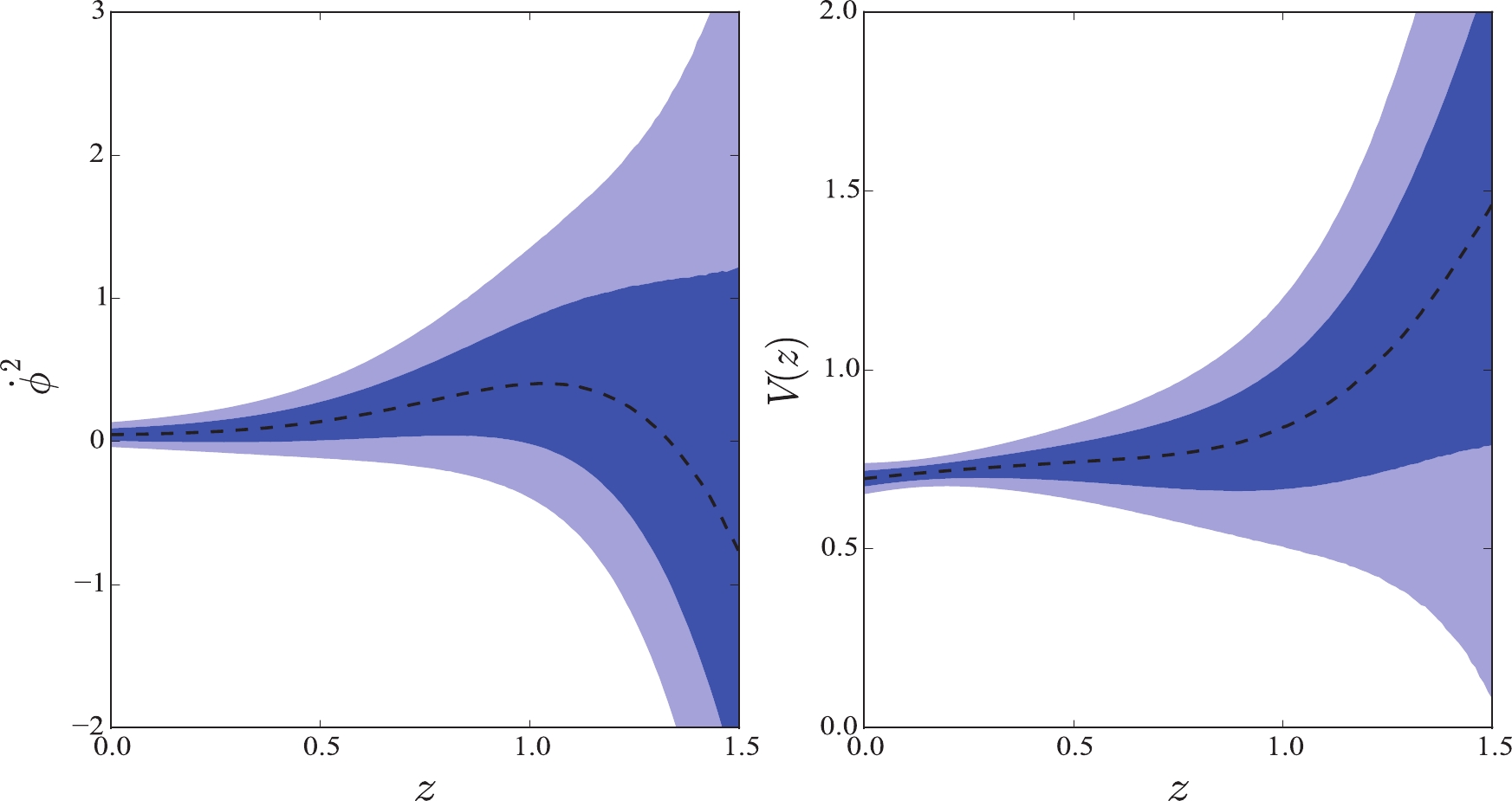
Figure 1. (color online) GP reconstruction in the quintessence field for JLA and
$ H(z) $ data with Hubble constant$ H_0 = 73.24 \pm 1.74 $ km s$ ^{-1} $ Mpc$ ^{-1} $ .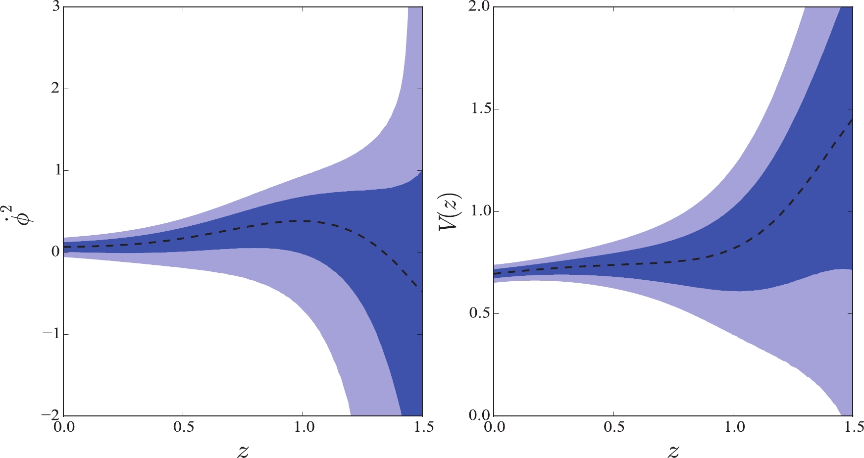
Figure 2. (color online) GP reconstruction in the tachyon field for JLA and
$ H(z) $ data with Hubble constant$ H_0 = 73.24 \pm 1.74 $ km s$ ^{-1} $ Mpc$ ^{-1} $ .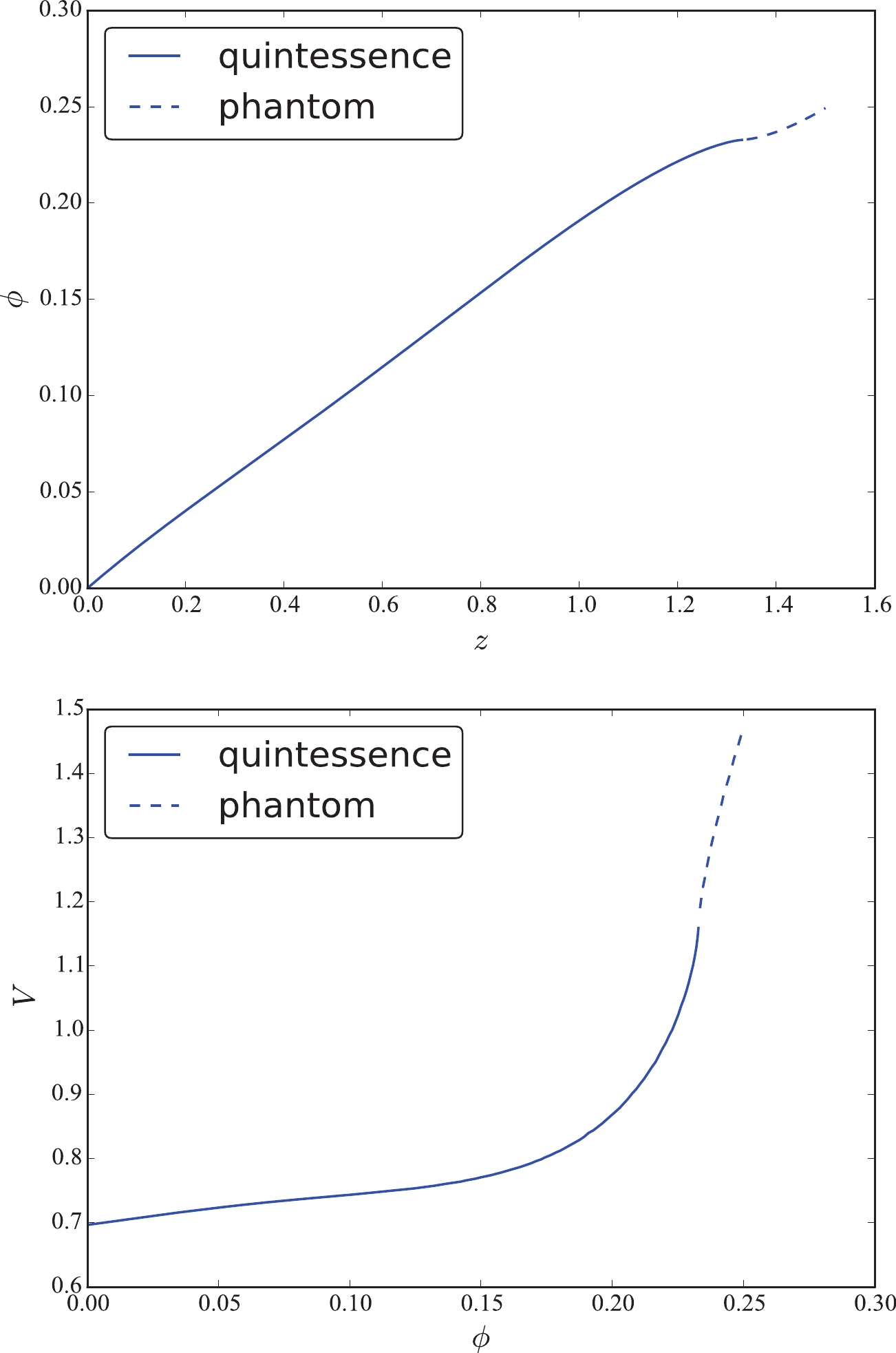
Figure 3. (color online) Field
$ \phi (z) $ and potential$ V(\phi) $ from their mean values for JLA and$ H(z) $ data with Hubble constant$ H_0 = 73.24 \pm 1.74 $ km s$ ^{-1} $ Mpc$ ^{-1} $ .$ 2.\;\; H_0=69.6 \pm 0.7 \; {\rm {km}} \;{\rm s} ^{-1} {\rm {Mpc}} ^{-1} $

In this prior, the JLA and
$ H(z) $ data present a slightly different reconstruction on these scalar fields.In Fig. 4, we plot the reconstructions in the quintessence field. First, compared with the reconstructions in Fig. 1, note that the function
$ \dot{\phi}^2 $ also increases first and then decreases with increasing redshift. Second, we found that mean values of the function$ \dot{\phi}^2 >0 $ , which means that the quintessence scalar field is favored to a certain degree. This situation is different from the above reconstruction. However, we must pay special attention to the fact that it cannot prevent the condition$ \dot{\phi}^2 < 0 $ at higher redshift within 68% confidence level. That is, considering the uncertainties of$ \dot{\phi}^2 $ , the quintom field is still a favourite model. This result is consistent with the reconstruction in$ H_0 = 73.24 \pm 1.74 $ km s$ ^{-1} $ Mpc$ ^{-1} $ . Finally, the reconstruction of$ V(z) $ shows that the data present an increasing potential. In particular, for redshift$ z \gtrsim 1 $ , it increases sharply. At redshift$ z = 0 $ , we have a model-independent estimation$ V_0 = 0.71 $ , which is similar to the above reconstruction.
Figure 4. (color online) GP reconstruction in the quintessence field for JLA and
$ H(z) $ data with Hubble constant$ H_0 = 69.6 \pm 0.7 $ km s$ ^{-1} $ Mpc$ ^{-1} $ .In Fig. 5, we plot the reconstructions in the tachyon field. We found that the data present a similar reconstruction to the quintessence field. That is, mean values of the function
$ \dot{\phi}^2 $ are also positive. A slight difference is that the potential$ V(z) $ decreases first and then increases. Within 68% confidence level, the function$ \dot{\phi}^2 < 0 $ is still supported by the data. Thus, the tachyon field cannot be convincingly favored by the data.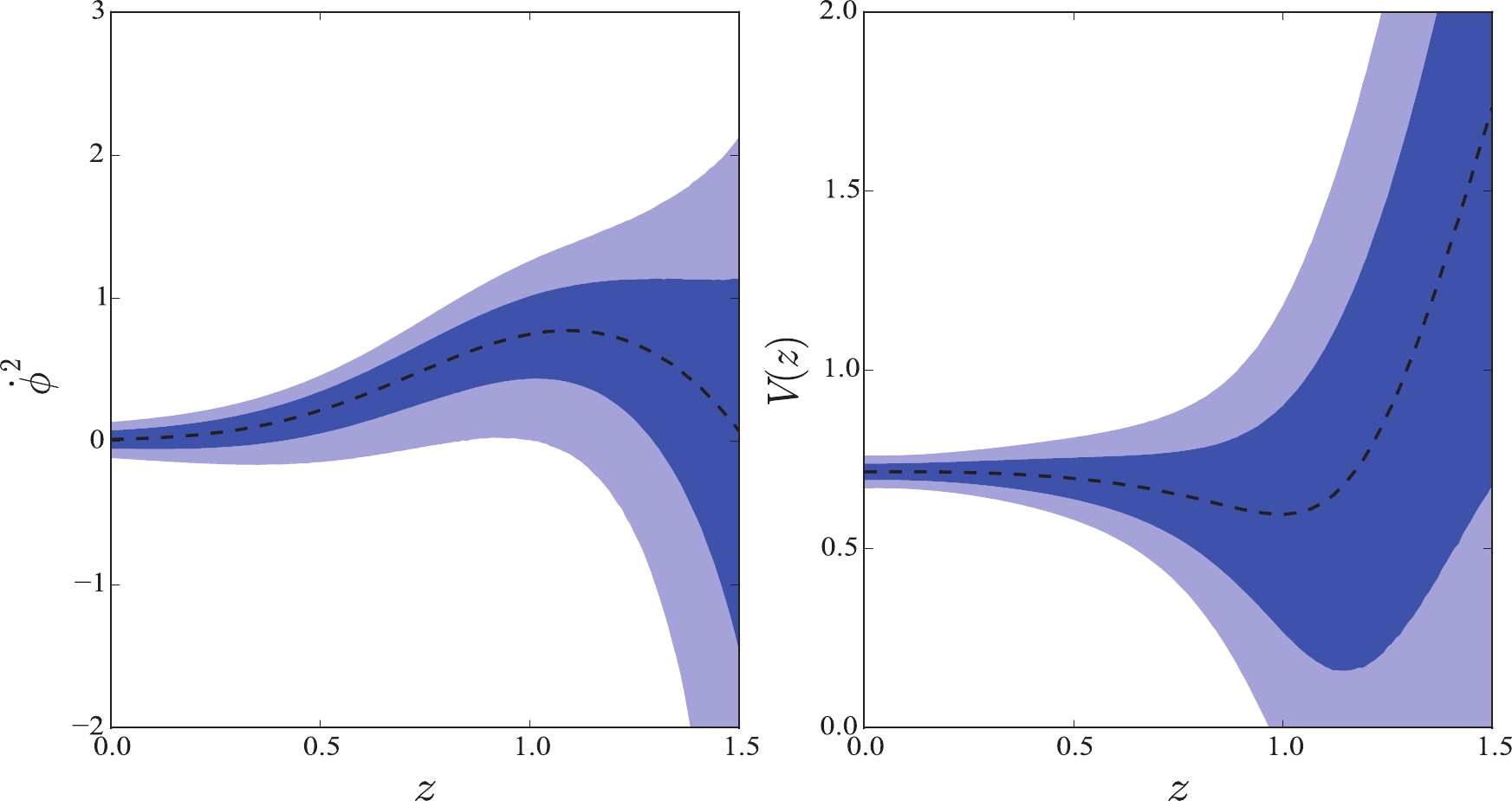
Figure 5. (color online) GP reconstruction in the tachyon field for JLA and
$ H(z) $ data with Hubble constant$ H_0 = 69.6 \pm 0.7 $ km s$ ^{-1} $ Mpc$ ^{-1} $ .In Fig. 6, we plot the scalar field
$ \phi (z) $ and potential$ V(\phi) $ using their mean values. This plot shows that the field$ \phi (z) $ also increases in the two models. However, in the middle redshift, they evolve slightly differently. For the initial value of potential, the data present the same value,$ V_0 = 0.71 $ , as in the quintessence field. Concerning the potential$ V(\phi) $ , the values are the same for the field$ \phi <0.10 $ . However, in the middle region, they present a significant difference. Therefore, the potential$ V(\phi) $ in these two fields may reflect different models.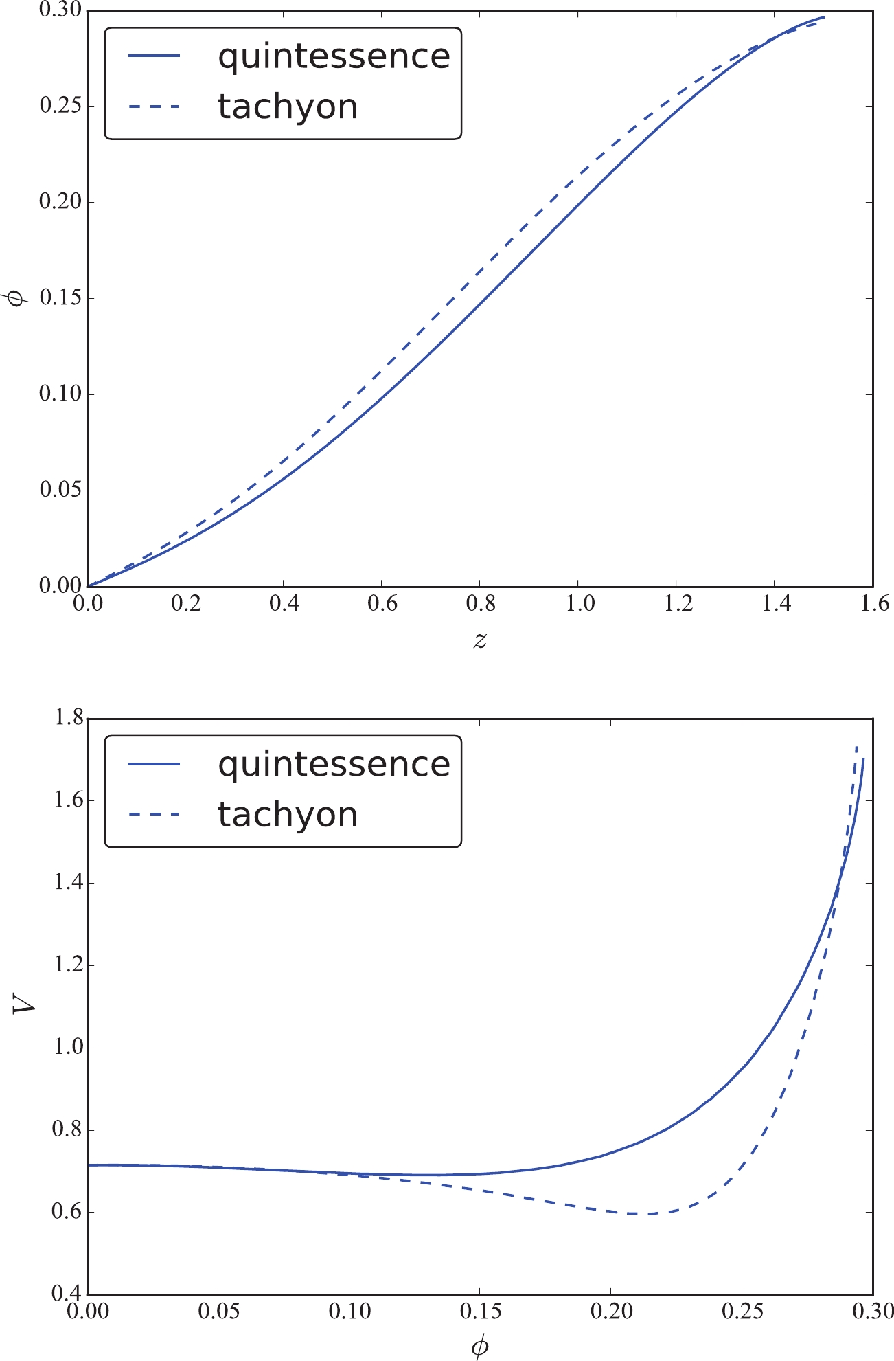
Figure 6. (color online) Field
$ \phi (z) $ and potential$ V(\phi) $ from their mean values for JLA and$ H(z) $ data with Hubble constant$ H_0 = 69.6 \pm 0.7 $ km s$ ^{-1} $ Mpc$ ^{-1} $ .Next, we fitted the function
$ V(\phi) $ in different fields; the results are listed in Table 1. We found that$ V(\phi) $ in the quintessence and tachyon fields are really different. Concerning the quintessence field, the mean values favor a double exponential function,$ V(\phi) = 0.7177 e^{-0.341 \phi} + 3.102 \times 10^{-4} e^{27.23 \phi} $ . For the tachyon field, a more complex double Gaussian function is required.JLA+ $ H(z) $ :

$ (H_0=73.24 \pm 1.74 ) $ 

quintom Exponential: $ V(\phi_q) = 0.7002 e^{0.5978 \phi_q} + 8.449 \times 10^{-6} e^{45.4 \phi_q} $ 

Gaussian : $V(\phi_p) = 1.501 e^{- \left(\frac{\phi_p - 0.2559}{0.03301}\right)^2 } + 0.2606 e^{- \left(\frac{\phi_p - 0.2307}{0.01163}\right)^2 }$ 

JLA+ $ H(z) $ :

$ (H_0=69.6 \pm 0.7) $ 

quintessence Exponential: $ V(\phi) = 0.7177 e^{-0.341 \phi} + 3.102 \times 10^{-4} e^{27.23 \phi} $ 

JLA+ $ H(z) $ :

$ (H_0=69.6 \pm 0.7) $ 

tachyon Gaussian : $V(\phi) = 1.192 \times 10^{3} e^{- \left(\frac{\phi - 0.6406}{0.1324}\right)^2 } + 0.7157 e^{- \left(\frac{\phi - 0.0302}{0.3793}\right)^2 }$ 

RSD: quintom Exponential: $ V(\phi_q) = 0.4981 e^{3.328 \phi_q} + 6.073 \times 10^{-7} e^{39.42 \phi_q} $ 

Gaussian : $V(\phi_p) = 1.951 e^{- \left(\frac{\phi_p - 0.4315}{0.1615}\right)^2 } + 0.4538 e^{- \left(\frac{\phi_p - 0.3107}{0.06524}\right)^2 }$ 

Table 1. Function
$ V(\phi) $ obtained by their mean values in different scalar fields for different observational data. -
In Fig. 7, the reconstruction in the quintessence field is plotted. We found that these results are similar to the reconstruction for JLA and
$ H(z) $ data. First, the function$ \dot{\phi}^2 $ from the background and RSD data presents a transformation from positive to negative in both cases, namely a direct transformation from the quintessence field to the phantom field. However, the difference with respect to the background data is that$ \dot{\phi}^2 $ from the RSD data changes more dramatically. Moreover,$ \dot{\phi}^2 $ at high redshift from the RSD data is completely negative within 68% confidence level. This indicates that the RSD data exhibit a higher potential to support the quintom model. Second, concerning the potential V, it is also an increasing function, but increases slower than that from the background data. The initial value of potential is$ V_0 = 0.50 $ , which is different from$ V_0 = 0.70 $ for the background data. Therefore, we hypothesize that the RSD data may represent a different scalar field model.
Figure 7. (color online) GP reconstruction in the quintessence field for RSD data.
In Fig. 8, we plot the reconstruction in the tachyon field. The mean values of the function
$ \dot{\phi}^2 $ also change from positive to negative, which is a case similar to Fig. 2. Considering their uncertainties,$ \dot{\phi}^2 > 0 $ cannot be ensured at high redshift within 68% confidence level. Therefore, we conclude that the tachyon field cannot be convincingly favored by the data. This determination is also extracted from the results for JLA and$ H(z) $ data. Concerning the potential V, it is also an increasing function. However, considering its errors, the potential V at high redshift is negative, which is invalid in terms of the definition in Eq. (8). In short, we conclude that the tachyon field is disadvantageous when it comes to describing the cosmic evolution.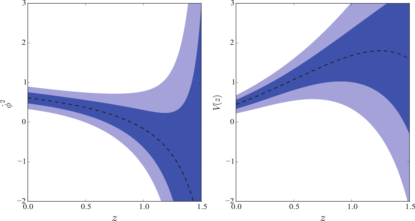
Figure 8. (color online) GP reconstruction in the tachyon field for RSD data.
In Fig. 9, we plot the field
$ \phi (z) $ and function$ V(\phi) $ using their mean values. As pointed out above, the function$ \dot{\phi}^2 $ in Fig. 7 cannot fulfill$ \dot{\phi}^2 > 0 $ at all redshifts. It changes from positive to negative at redshift$ z \sim 0.90 $ . Scalar fields also naturally change from the quintessence field to the phantom field, as shown in this figure. Similar to the above reconstruction from the background data, the field$ \phi (z) $ is also a monotone increasing function. To describe the reconstructed scalar field, we deemed it as a quintom field that changes from phantom field to quintessence field with the cosmic evolution. The plot shows that it is also a complicated model similar to that of Fig. 3. From Table 1, we found that$ V(\phi_q) $ must satisfy a double exponential function, and$ V(\phi_p) $ is a double Gaussian function, which is fully consistent with the reconstruction from the background data.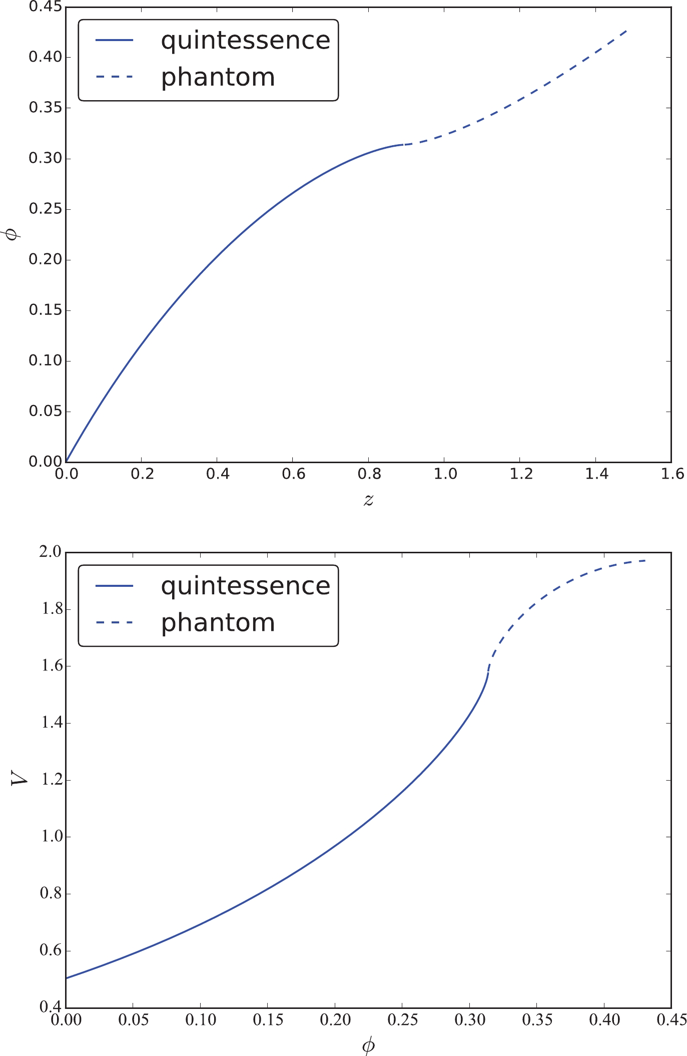
Figure 9. (color online) Field
$ \phi (z) $ and potential$ V(\phi) $ from their mean values for RSD data. -
In this study, a test with model-independence on the scalar field was put into operation to explore the source of dark energy, using the Gaussian processes approach. We used the combination of supernova data and
$ H(z) $ data, and growth rate data.Although we investigated the dark energy using the GP method in a previous study of ours [32], we must emphasize that it still has important physical significance. Compared with our previous study, the present one clearly shows which scalar field is the candidate for dark energy. According to the reconstruction results, we found that it is neither the quintessence field nor the phantom field. It is probably another substance, namely the quintom field. Moreover, the fitting of potential
$ V(\phi) $ is still beyond our imagination. It can provide an important reference on the scalar field study.In the past few years, the scalar field was studied via many parameterizations. The focus of attention was which template was the best dynamical description of dark energy. The research presented in this paper constitutes a template-free analysis. We not only reconfirmed that the dark energy must be dynamical but also reconstructed the potential over the scalar field.
According to the background data, we found that they do not favor a single quintessence field, phantom field, or tachyon field in the prior of
$ H_0 = 73.24 \pm 1.74 $ km s$ ^{-1} $ Mpc$ ^{-1} $ . Their mean values indicate that they favor a quintom field, which is a transformation between phantom field and quintessence field. The fitted potential$ V(\phi) $ in the quintessence field is a double exponential function, whereas$ V(\phi) $ in the phantom field is a double Gaussian function, as shown in Table 1. We also tested the effect from the Hubble constant and found that$ H_0 $ has a marked influence on the reconstruction. When considering their uncertainties, the reconstructions also favor the quintom field.Our study also solves another point. In a previous study [42], it was found that the tachyon models present phenomenology similar to that of canonical quintessence models. We found that they are really similar at low redshift (or small
$ \phi $ ). However, they also present an unnegligible difference at middle redshift, as shown in Fig. 6. Moreover, the background and RSD data reveal that the tachyon field is disadvantageous when it comes to describing the cosmic acceleration.According to the RSD data, a quintom field is also suitable. This determination is identical from the analysis conducted from the background data. Moreover, the RSD data are more potential to support the quintom model within 68% confidence level. Their mean values show that the potential
$ V(\phi) $ is fully consistent with the reconstruction from background data.Discussions about the dynamics of dark energy revolved around whether it evolved or not. Our analysis clearly reveals that the dark energy must be dynamical, regardless of considering background data, i.e., supernova and
$ H(z) $ data or perturbation data, i.e., RSD data. Moreover, the corresponding reconstructions favor the quintom field. In a recent study by Zhao et al. [ 7], the authors investigated the Kullback–Leibler divergence using the latest data, including CMB temperature and polarization anisotropy spectra, supernova, BAO from the clustering of galaxies and from the Lyman-$ \alpha $ forest, Hubble constant, and$ H(z) $ . The study reveals that a dynamical dark energy can moderate the Hubble constant tension. Moreover, it is preferred at a 3.5$ \sigma $ C.L. In addition, the forthcoming dark energy survey DESI++ can provide a decisive Bayesian evidence. In future work, we would like to incorporate more observational data on the study of the scalar field to conduct a clearer analysis on cosmic dynamics.Another point we must emphasize is the importance of the Hubble constant. We note that it has a notable influence on the determination of dark energy dynamics. The tension in
$ H_0 $ raised great concern. Some previous studies [68, 69] concluded that it may be a signature of new physics. To date, its measurement window spanned from traditional cepheids, tip of the red giant branch, SNIa, surface brightness fluctuations, masers, and gravitational lens time delays, to fashionable gravitational-waves [70]. The detection of GW170817 involved the merging of a binary neutron-star system with a strong signal. The identification of its host galaxy implied a completely independent and consistent determination with existing measurements [71]. Moreover, it can also be measured with neutron star black hole mergers from advanced LIGO and Virgo [72]. The future multi-messenger astronomy will enable the$ H_0 $ and cosmic dynamics to be constrained with high precision. -
We thank the anonymous referee whose suggestions greatly helped us improve this paper. M.-J. Zhang would like to thank Shulei Ni, De-Liang Wu, Hua Zhai, and Xiao Wang for valuable discussions.
Observational constraint on the dark energy scalar field
- Received Date: 2020-01-28
- Available Online: 2021-04-15
Abstract: In this paper, we study three scalar fields, namely the quintessence, phantom, and tachyon fields, to explore the source of dark energy via the Gaussian processes method from the background and perturbation growth rate data. The corresponding reconstructions suggest that the dark energy should be dynamical. Moreover, the quintom field, which is a combination of the quintessence and phantom fields, is powerfully favored by the reconstruction. The mean values indicate that the potential


 DownLoad: