


 Abstract
 HTML
HTML Reference
 Related
 PDF
PDF


-
After the discovery of the SM-like Higgs boson at the Large Hadron Collider (LHC) [1,2], particle physicists paid more attention to the investigation of the properties of the SM-like Higgs boson. With the theoretical and experimental uncertainties, most of the results are consistent with the SM predictions [3,4].
To verify the predictions of the SM, it is not enough to check the strength of interactions between the SM-like Higgs boson and other SM particles. Researchers need to investigate the Lorentz structure and the coupling constants associated with each possible Lorentz structure. For example, the generic form of the interaction between the SM-like Higgs boson and the SM fermions is
$ \begin{aligned}[b]& {\cal{L}}_{Y_f} = -y_fh\bar \psi_f(\cos\alpha_f+{\rm i}\gamma_5\sin\alpha_f)\psi_f, \\& y_f>0,\; \alpha_f\in (-\pi,\pi],\; f = e,\mu,\tau,u,d,c,s,t,b. \end{aligned} $

(1) In the SM, we have
$ y_f = y_f^{{\rm{SM}}} = m_f/(\sqrt2v) $ ($ v = 174 $ GeV is the vacuum expectation of the SM Higgs field) and$ \alpha_f = 0 $ for massive SM fermions. Although the phase angle$ \alpha_f $ could be removed by a redefinition of the fermion field$ \psi_f{\rightarrow} \psi_f^\prime = {\rm e}^{-{\rm i}\alpha_f\gamma_5/2}\psi_f $

(2) for massless fermions, such redefinition will not work for massive fermions because their phases have been fixed by the mass
$ m_f\in\mathbb{R}^+ $ in the Lagrangian${\bar \psi _f}({\rm i}{\not\!\! D} - {m_f}){\psi _f}$ of free fermion fields. Thus, either$ y_f\neq m_f/(\sqrt 2 v) $ or$ \alpha_f\neq0 $ will be the evidence of the new physics (NP) beyond the SM.Due to the large value of
$ y_t $ , the measurement of the phase angle in the top-Higgs interaction$ \alpha_t $ is relatively easy and has been proposed in a number of studies (for example, see [5-21]). However, the$ \alpha_f $ values of the down-type fermions are also very interesting and important from a theoretical point of view. A well known example is the "wrong-sign limit" in some types of the two-Higgs-doublet model (2HDM). Without any other deviation from the predictions of the SM,$ \alpha_b\approx\pi $ (because$ y_b $ is the largest$ y_f $ in the down-type fermions,$ \alpha_b $ is probably the easiest one to be measured) is a strong hint for these types of NP models.Much effort has been made to measure
$ \alpha_b $ . Although the direct measurement is very challenging at the LHC [22,23], it can be measured indirectly in electric dipole moment (EDM) experiments [24-26] or at the LHC with additional model-dependent assumptions (e.g., in the frame of 2HDM [27-36]). The constraints on the indirect measurement are strong but suffer from the potential contributions of exotic degrees of freedom in the NP. For this reason, a direct, model-independent measurement is still necessary.In this work, we investigate the possibility of measuring
$ \alpha_b $ directly and model-independently at a future Higgs factory. -
To the leading order, the effective Lagrangian in Eq. (1) modifies the
$ h{\rightarrow} b\bar b $ decay width to$ \Gamma(h{\rightarrow} b\bar b) = \Gamma(h{\rightarrow} b\bar b)^{{\rm{SM}}}\left(\frac{y_b}{y_b^{{\rm{SM}}}}\right)^2\left(\cos^2\alpha_b+\beta_b^{-2}\sin^2\alpha_b\right), $

(3) where
$ \beta_b\equiv \sqrt{1-4m_b^2/m_h^2} $ . The precise measurement of the decay branching ratio can only constrain the combination$ \begin{aligned}[b]& \left(\frac{y_b}{y_b^{{\rm{SM}}}}\right)^2\left(\cos^2\alpha_b+\beta_b^{-2}\sin^2\alpha_b\right)\\ \sim&\left(\frac{y_b}{y_b^{{\rm{SM}}}}\right)^2\left(1+\frac{4m_b^2}{m_h^2}\sin^2\alpha_b\right)\\ =& \left(\frac{y_b^{{\rm{SM}}}+\delta y_b}{y_b^{{\rm{SM}}}}\right)^2\left(1+0.0058\sin^2\alpha_b\right)\\ \sim&1+2\left(\frac{\delta y_b}{y_b^{{\rm{SM}}}}\right)+\left(\frac{\delta y_b}{y_b^{{\rm{SM}}}}\right)^2+0.0058\sin^2\alpha_b \end{aligned} $

(4) of
$ y_b $ and$ \alpha_b $ , in which the contribution from$ \alpha_b $ is numerically small. Even if we keep$ y_b = y_b^{{\rm{SM}}} $ , the partial width will be in the region of$ \Gamma(h{\rightarrow} b\bar b)^{{\rm{SM}}} $ (1.0029±0.29%). This small discrepancy is just below the sensitivity at Higgs factories [37-39]. Thus, we have to look for other kinematic variables that are sensitive to$ \alpha_b $ .To measure
$ \alpha_b $ , we consider the interference effect in the$ h{\rightarrow} \bar bbg $ process, whose Feynman diagrams are shown in Fig. 1.
Figure 1. The Feynman diagrams that are used to measure the relative sign between the bottom-quark Yukawa coupling constant and the weak interaction gauge coupling constant.
The transition amplitude can be written as
$ {\cal{M}} = {\rm e}^{\pm {\rm i}\alpha_b}{\cal{M}}_1+{\cal{M}}_2 , $

(5) where
$ {\cal{M}}_1 $ represents the contribution from Feynman diagrams (a) and (b),$ {\cal{M}}_2 $ represents the contribution from Feynman diagram (c), both of which are$ \alpha_b $ -independent. In Eq. (5), the sign before the phase angle$ \alpha_b $ depends on the chirality configuration of the$ b\bar b $ in the final state.Because the
$ hb\bar b $ vertex flips the chirality of the fermion line, while the$ gb\bar b $ does not, if the$ b $ -quark is massless, the interference term will vanish. It can only appear when the$ b $ -quark is massive, in which case the chirality is not a good quantum number. The terms$ {\cal{M}}_1 $ and$ {\cal{M}}_2 $ can be non-zero at the same time due to the mass insertion effect. The technical analysis of this can be understood easily. Since in the massless limit the chiral symmetry is restored, and one can remove$ \alpha_b $ with the symmetry transformation of Eq. (2),$ \alpha_b $ should not have any observable effect in this limit. Thus, any observable effect of$ \alpha_b $ is expected to be proportional to$ m_b $ .Our next aim is to find the phase space region where the interference effect is large. This will guide us to design a suitable observable and cuts. The relative size of the interference effect can be described by the ratio between the interference term and the non-interference terms
$ \frac{{\rm e}^{\pm {\rm i}\alpha_b}{\cal{M}}_1{\cal{M}}_2^*+ {\rm e}^{\mp {\rm i}\alpha_b}{\cal{M}}_1^*{\cal{M}}_2}{|{\cal{M}}_1|^2+|{\cal{M}}_2|^2} = 2\cos(\pm\alpha_b+\phi)\frac{|{\cal{M}}_1|\cdot|{\cal{M}}_2|}{|{\cal{M}}_1|^2+|{\cal{M}}_2|^2}, $

(6) where
$ \phi $ is phase angle of$ {\cal{M}}_1{\cal{M}}_2^* $ . As a matter of fact, we can only measure$ \alpha_b+\phi $ with this process. However, the effective$ hgg $ vertex$ \left(\frac{\alpha_s}{12\sqrt 2\pi v}+\frac{c_{hgg}}{\Lambda}\right)hG_{\mu\nu}^aG^{a,\mu\nu}+\frac{\tilde c_{hgg}}{\Lambda}hG_{\mu\nu}^a\tilde G^{a,\mu\nu} $

(7) can be independently and precisely measured at the LHC [40-44], so that the model dependence from this part is low, which is another advantage of this process. In our work, we choose the SM value,
$ c_{hgg} = \tilde c_{hgg} = 0 $ in the low energy limit. To obtain a significant modulation effect, we need to find the phase space region where$ |{\cal{M}}_1|\cdot |{\cal{M}}_2|/(|{\cal{M}}_1|^2+ |{\cal{M}}_2|^2) $ is large. It is obvious that this quantity reaches its maximal value when$ |{\cal{M}}_1| = |{\cal{M}}_2| $ . Because$ y_b> \alpha_sm_h/(12\sqrt 2\pi v) $ , generically we have$ |{\cal{M}}_1|>|{\cal{M}}_2| $ . Therefore, we should focus on the phase space region where$ {\cal{M}}_2 $ is more enhanced. Certainly, it is the region where$ b\bar b $ is collinear, because$ {\cal{M}}_2 $ has a large QCD collinear divergence in this region and is largely enhanced, while$ {\cal{M}}_1 $ has no QCD divergence in the region. Guided by this analysis, we define an observable as$ \zeta_{H}\equiv\frac{2E_{b_1}E_{b_2}}{E_{b_1}^2+E_{b_1}^2}\cos\theta_{b_1b_2}, $

(8) where
$ E_{b_i} $ is the energy of the ith$ b $ -jet in the Higgs rest frame, and$ \theta_{b_1b_2} $ is the open angle between the two$ b $ -jets in the Higgs-rest frame.A straightforward calculation gives the differential partial decay width (to the order of
$ m_b $ )①$ \begin{aligned}[b] \frac{{\rm d}^2\Gamma}{{\rm d}x_{13}{\rm d}x_{23}} =& \frac{y_b^2m_h\alpha_s}{4\pi^2}\biggl\{\Pi_{11}(x_{13},x_{23})+2\Pi_{12}(x_{13},x_{23})\\& \times\frac{m_b}{m_h}r\cos\alpha_b+\Pi_{22}(x_{13},x_{23})r^2\}, \end{aligned} $

(9) $ \Pi_{11}(x_{13},x_{23}) = \frac{1+(1-x_{13}-x_{23})^2}{x_{13}x_{23}}, $

(10) $ \Pi_{12}(x_{13},x_{23}) = \frac{(x_{13}+x_{23})(x_{13}-x_{23})^2+4x_{13}x_{23}}{x_{13}x_{23}(1-x_{13}-x_{23})}, $

(11) $ \Pi_{22}(x_{13},x_{23}) = \frac{x_{13}^2+x_{23}^2}{(1-x_{13}-x_{23})}, $

(12) where
$ r\equiv \frac{\alpha_s}{6\sqrt2\pi y_b}\left(\frac{m_h}{v}\right)\sim\frac{1}{4}, $

(13) $ x_{13} = (p_b+p_g)^2/m_h^2 $ , and$ x_{23} = (p_{\bar b}+p_g)^2/m_h^2 $ , in which$ p_b,p_{\bar b} $ , and$ p_g $ are the four momentum of the bottom-quark, the anti-bottom-quark, and the gluon in the Higgs-rest frame, respectively. In this formula, the term$ \Pi_{ij} $ is from the amplitude square term$ ({\cal{M}}_i^*{\cal{M}}_j+{\cal{M}}_i{\cal{M}}_j^*)/(1+\delta_{ij}) $ . It is easy to verify our intuitive analysis with this formula. -
In this section, we investigate the collider phenomenology at future Higgs factories [37,39]. The lepton collider is designed to run with 240 GeV collision energy with roughly 5 ab−1 integrated luminosity②. Some of them also have a plan to run with 365 GeV collision energy and roughly 1.5 ab−1 integrated luminosity [39]. Here, we provide the results of parton level collider simulation for both 240 GeV and 365 GeV lepton colliders.
-
We generate parton level signal and background events for a 240 GeV
$ e^+e^- $ collider using MadGraph_aMC@NLO [45] with the initial state radiation (ISR) effects [46]. To include the NNLO corrections to the cross section, the total cross section of$ e^+e^-{\rightarrow} Zh $ is rescaled to the value suggested in [47-49]. We analyze both leptonic and hadronic decay modes of the$ Z $ boson. The interference effect between the Higgs strahlung process and the$ Z $ -boson fusion process in the$ e^+e^- $ decay case of$ Z $ boson is considered in our analysis. The jet algorithm is the$ ee\_{\rm{kt}} $ (Durham) algorithm in which the distance between objects$ i $ and$ j $ is defined as [50]$ d_{ij}\equiv2\left(1-\cos\theta_{ij}\right)\frac{\min\left(E_i^2,E_j^2\right)}{s}, $

(14) where
$ s $ is the square of the center-of-mass frame energy,$ E_{i} $ is the energy of the ith jet, and$ \theta_{ij} $ is the angle opened by the ith and jth jet.We add pre-selection cuts when we generate the parton level event
$ \begin{aligned}& |\eta_{{\rm jet},\ell^\pm}|\!<\!2.3,\quad \Delta R_{ij}\!>\!0.1,\quad \Delta R_{i\ell}\!>\!0.2,\\& E_{\rm jet}\!>\!10{{\rm{GeV}}},\quad E_{\ell^\pm}\!>\!5{{\rm{GeV}}}. \end{aligned} $

The parameters of the smearing effects for different particles are chosen to be [37]
$ \begin{aligned}[b] \frac{\sigma(E_{\rm jet})}{E_{\rm jet}} =& \frac{0.60}{\sqrt{E_{\rm jet}/{{\rm{GeV}}}}}\oplus 0.01,\\ \frac{\sigma(E_{e^\pm,\gamma})}{E_{e^\pm,\gamma}} =& \frac{0.16}{\sqrt{E_{e^\pm,\gamma}/{{\rm{GeV}}}}}\oplus 0.01,\\ \sigma\left(\frac{1}{p_{{\rm{T}},\mu^\pm}}\right) =& 2\times10^{-5}\; {{\rm{GeV}}}^{-1}\oplus\frac{0.001}{p_{\mu^\pm}\sin^{3/2}\theta_{\mu^\pm}}, \end{aligned} $

-
After adding the smearing effects, we require that the objects satisfy③
$ \begin{aligned}[b]& |\cos\theta_{{\rm jet},\ell^\pm}|<0.98,\; d_{ij}>0.002, E_{\rm jet}>15{{\rm{GeV}}}, \\& \Delta R_{i\ell^\pm}>0.2,\; E_{\ell^\pm}>10{{\rm{GeV}}}. \end{aligned} $

The b-tagging efficiency is chosen to be 80%, while the mis-tagging rate from charm jet (light jet) is 10% (1%). After the preselection cuts, we require that the signal events contain exactly two b-tagged jets, one non-b jet, a pair of opposite sign same flavor charged leptons, and
$ \begin{array}{l} |m_{\mu^+\mu^-}-m_Z|<10{{\rm{GeV}}},\; \; |m_{e^+e^-}-m_Z|<15{{\rm{GeV}}},\\ \theta_{\ell^+\ell^-}>80^\circ,\; \; \; \; {{\not\!\! E}_{{\rm{T}}}}<10{{\rm{GeV}}},\\ 124.5{{\rm{GeV}}}<m_{{\rm{r}}}(\mu^+\mu^-)<130{{\rm{GeV}}},\; {{\rm{for}}}\; \mu^+\mu^-\; {{\rm{channel}}},\\ 118\; {{\rm{GeV}}}<m_{{\rm{r}}}(e^+e^-)<140{{\rm{GeV}}},\; {{\rm{for}}}\; e^+e^-\; {{\rm{channel}}}, \end{array} $

where the recoil mass
$ m_{{\rm{r}}}(ij) $ is defined as$ m_{{\rm{r}}}(ij)\equiv \sqrt{ s-2\sqrt s (E_i+E_j)+(p_i+p_j)^2}. $

(15) The dominant SM background processes for
$ Z{\rightarrow}\ell^+\ell^- $ channel is$ \begin{array}{l} e^+e^-\;\;{\rightarrow}\;\; \ell^+\ell^-b\bar b j\\ e^+e^-\;\;{\rightarrow}\;\; \ell^+\ell^-c\bar c j\\ e^+e^-\;\;{\rightarrow}\;\; \ell^+\ell^-j j j\\ e^+e^-\;\;{\rightarrow}\;\; \ell^+\ell^- h({\rightarrow} c\bar c j)\\ e^+e^-\;\;{\rightarrow}\;\; \ell^+\ell^- h({\rightarrow} j j j) \end{array} $

The kinematic cut on the recoil mass of
$ \ell^+\ell^- $ can remove most of the background events from the first three SM processes, while the last two can pass this cut. However, the last two background events will be suppressed by the charm-jet and light jet mistagging rate.In our analysis, the 4-momentum of the Higgs boson is reconstructed by summing the 4-momentum of the three jets from the Higgs boson decay but not the recoil momentum of the dilepton system. When the two
$ b $ -jets from the Higgs boson decay are nearly collinear and the$ b\bar b $ -system and the gluon jet from the Higgs boson decay are nearly back-to-back,$ \zeta_H $ goes to its maximum value, +1. In Fig. 2, we show the$ \zeta_H $ distributions for the SM backgrounds and the signal with different values of$ \alpha_b $ . The behavior of the distribution, especially in the last several bins, is consistent with our intuitive analysis.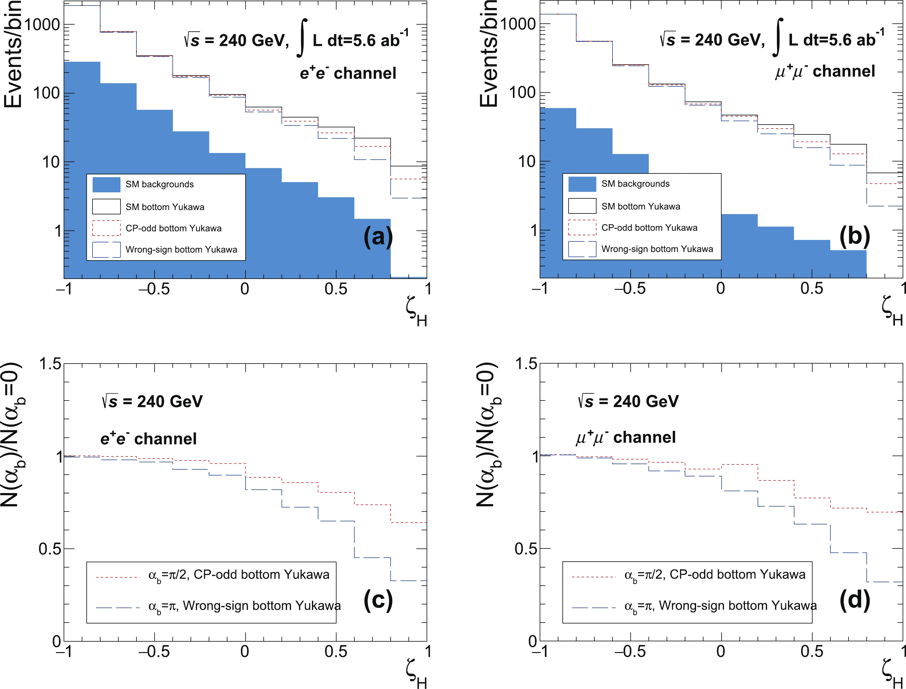
Figure 2. (color online) The
$\zeta_H$ distributions for the SM background, the SM bottom-quark Yukawa interaction ($\alpha_b = 0$ ), bottom-quark Yukawa interaction with CP-odd scalar ($\alpha_b = \pi/2$ ), and the wrong-sign bottom-quark Yukawa interaction ($\alpha_b = \pi$ ) at 240 GeV Higgs factory with 5.6 ab−1 integrated luminosity. (a) The$\zeta_H$ distribution of$Z{\rightarrow} e^+e^-$ channel; (b)$\zeta_H$ distribution of$Z{\rightarrow} \mu^+\mu^-$ channel; (c) ratio of the event rates with respect to the SM case ($\alpha_b = 0$ ) of$Z{\rightarrow} e^+e^-$ channel; (d) ratio of the event rates with respect to the SM case ($\alpha_b = 0$ ) of$Z{\rightarrow} \mu^+\mu^-$ channel. -
Although the analysis is more complicated than the channels in which the
$ Z $ boson decays leptonically, the branching ratio of the hadronic decay mode of the$ Z $ boson is much larger. Thus, it is worth making the effort to include the information from this channel. After adding the smearing effects, we require that the objects satisfy$ |\cos\theta_i|<0.98,\; d_{ij}>0.002, E_{\rm jet}>15{{\rm{GeV}}}, {{\not\!\! E}_{{\rm{T}}}}<10{{\rm{GeV}}}. $

To avoid an estimation that is too aggressive in the jet-rich environment, for this mode, we assume that the
$ b $ -tagging efficiency is 60% (lower than that of the leptonic channel), while the mis-tagging rate from charm jet (light jet) is 10% (1%). After the preselection cuts, we require that the signal events contain at least two$ b $ -tagged jets and five jets in total. To reconstruct the Higgs boson and the$ Z $ boson, we use the likelihood method. The distributions of the truth reconstructed$ Z $ -boson mass, the Higgs boson mass, the$ Z $ -boson recoil mass, and the Higgs boson recoil mass are$ L_Z(m) = P(m;91.0{{\rm{GeV}}},6.19{{\rm{GeV}}}), $

(16) $ L_h(m) = P(m;125.3{{\rm{GeV}}},6.54{{\rm{GeV}}}), $

(17) $ L_{rZ}(m) = P(m;126.7{{\rm{GeV}}},8.43{{\rm{GeV}}}), $

(18) $ L_{rh}(m) = P(m;93.0{{\rm{GeV}}},10.56{{\rm{GeV}}}), $

(19) respectively, where
$ P(x;\mu,\sigma) = \frac{1}{\sqrt{2\pi}\sigma}\exp\left[-\frac{(x-\mu)^2}{2\sigma^2}\right] $

(20) is the standard probability distribution function (p.d.f) of the normal distribution. We minimize a discriminator defined as
$\begin{aligned}[b] \Delta =& -2\ln L_Z(m_{i_1i_2})-2\ln L_h(m_{i_3i_4i_5})\\& -2\ln L_{rZ}(m_{{{\rm{recoil}}}}(i_1i_2))-2\ln L_{rh}(m_{{\rm{recoil}}}(i_3i_4i_5))\\& -70B({i_3})-70B({i_4})+100B({i_5}), \end{aligned}$

(21) where
$ i_1,\cdots,i_5 $ is a permutation of the five jets,$ m_{i\cdots j} $ is the invariant mass of the ith,$ \cdots $ , and the jth jet,$ m_{{\rm{recoil}}}(i\cdots j) $ is the recoil mass of the ith,$ \cdots $ , and the jth jet, and$ B(i) $ is 1 (0) if the ith jet is tagged (not) to be a$ b $ -jet. If$ i_1,\cdots,i_5 $ gives the minimum$ \Delta $ , we treat$ j_{i_1},j_{i_2} $ as jets from the$ Z $ decay,$ j_{i_3},j_{i_4} $ as the$ b $ -jets from the Higgs boson decay, and$ j_{i_5} $ as the gluon from the Higgs boson decay. For the signal events, the reconstruction efficiency is ~80%. We require that there are at least two$ b $ -jets in$ j_{i_3},j_{i_4} $ and$ j_{i_5} $ ,$ \Delta<45 $ , and$ 120^\circ<\theta_{i_1i_2}<150^\circ $ .The dominant SM background processes for the
$ Z{\rightarrow} jj $ channel are$ \begin{array}{l} e^+e^-\;\;{\rightarrow}\;\; j j j j j\\ e^+e^-\;\;{\rightarrow}\;\; j j h({\rightarrow} c\bar c j)\\ e^+e^-\;\;{\rightarrow}\;\; j j h({\rightarrow} j j j). \end{array} $

After the reconstruction, we can obtain the
$ \zeta_H $ distribution, which is shown in Fig. 3; we show the$ \zeta_H $ distributions for the residue SM backgrounds and the signal with different values of$ \alpha_b $ .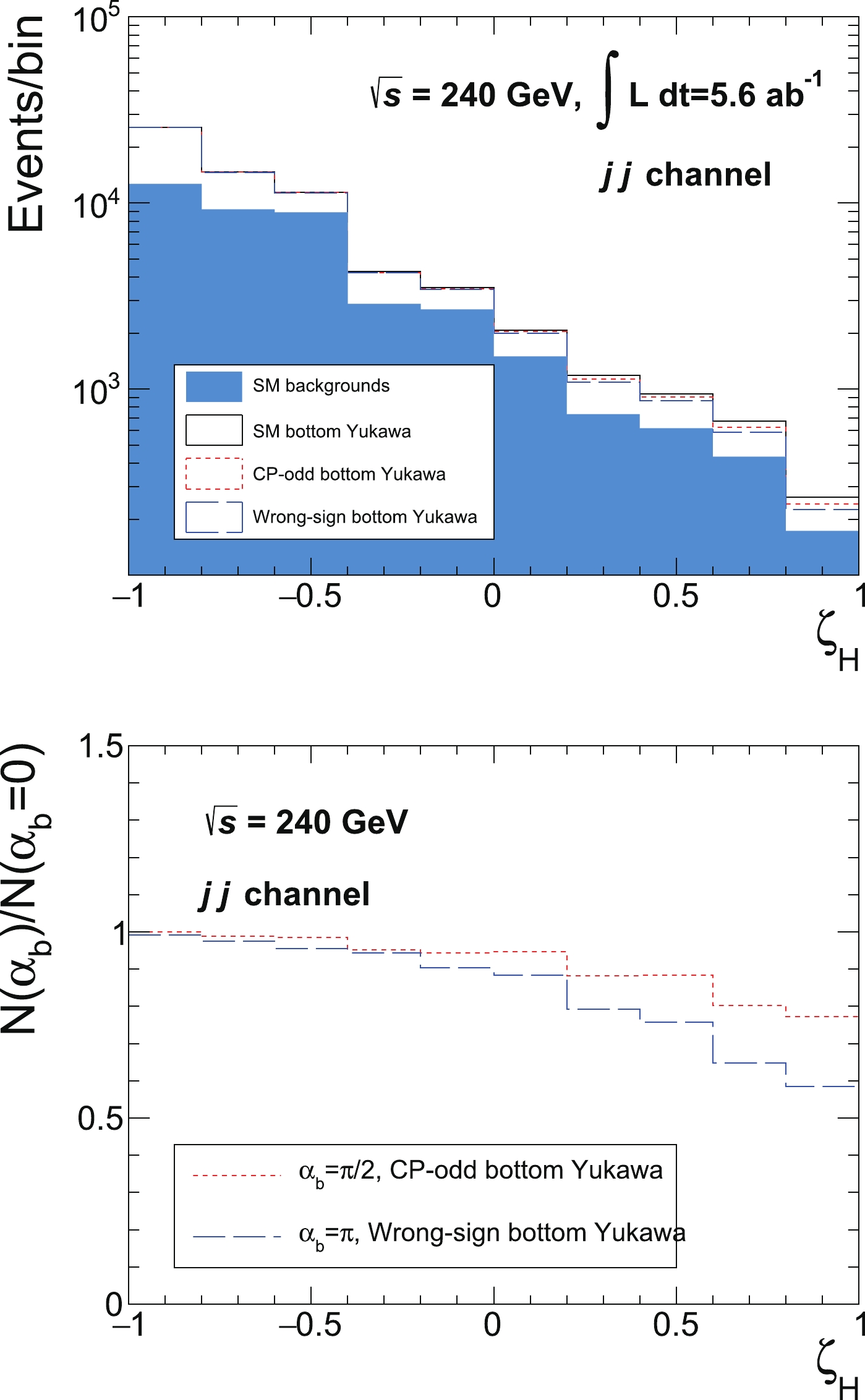
Figure 3. (color online) The
$\zeta_H$ distributions for the SM background, the SM bottom-quark Yukawa interaction ($\alpha_b = 0$ ), bottom-quark Yukawa interaction with CP-odd scalar ($\alpha_b = \pi/2$ ), and the wrong-sign bottom-quark Yukawa interaction ($\alpha_b = \pi$ ) at 240 GeV Higgs factory with 5.6 ab−1 integrated luminosity for hadronic decaying$Z$ . Upper panel: the$\zeta_H$ distribution; Lower panel: the ratio of the event rates with respect to the SM case ($\alpha_b = 0$ ). -
We define the binned likelihood function by
$ L(\mu,\alpha)\equiv\prod\limits_{i = 1}^{N_{{\rm{bin}}}}\frac{\left[\mu s(\alpha)_i+b_i\right]^{n_i}}{n_i!} {\rm e}^{-\mu s(\alpha)_i-b_i}, $

(22) where
$ \mu $ is the signal strength,$ s(\alpha)_i $ is the number of signal events in the ith bin under the hypothesis$ \alpha_b = \alpha $ ,$ b_i $ is the number of SM background events in the ith bin, and$ n_i $ is the number of total events observed in the ith bin. Thus, under the assumption that$ \alpha_b = \alpha_0 $ , the logarithm of the ratio of the likelihood function will be$\begin{aligned}[b] -2\Delta\log L \equiv & -2\log\frac{L(\mu,\alpha)}{L(\mu_0,\alpha_0)}\\ =& -2\sum\limits_{i = 1}^{N_{{\rm{bin}}}}\biggl\{\mu_0s(\alpha_0)_i-\mu s(\alpha)_i+[\mu_0 s(\alpha_0)_i+b_i]\\& \times\log\left(\frac{\mu s(\alpha)_i+b_i}{\mu_0 s(\alpha_0)_i+b_i}\right)\}. \end{aligned}$

(23) With
$ -2\Delta\log L = q^2 $ , we can estimate the$ q\sigma $ confidence level (C.L.) exclusion region under the SM hypothesis$ \alpha_b = 0 $ . We present the result in the complex plane for the complex parameter defined by$ Y_b\equiv y_b{\rm e}^{{\rm i}\alpha_b}/y_b^{{\rm{SM}}} $ . The result is shown in Fig. 4.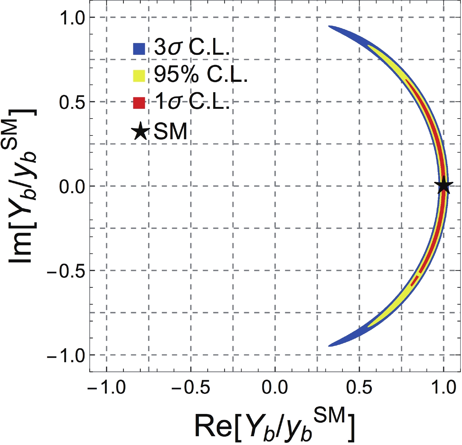
Figure 4. (color online) The constraint for
$Y_b$ at 240 GeV Higgs factory with 5.6 ab−1 integrated luminosity after combining the leptonic and hadronic decaying$Z$ channels.We can estimate the measurement uncertainty
$ \delta\alpha $ for arbitrary$ \alpha_0 $ by solving$ -2\log\frac{L(\hat \mu,\alpha_0+\delta\alpha)}{L(1,\alpha_0)} = 1, $

(24) where
$ \hat\mu $ is chosen by minimizing the quantity on the left-hand side of Eq. (24). The result is shown in Fig. 5. The larger uncertainty for$ \alpha_b{\rightarrow}0 $ and$ \alpha_b{\rightarrow}\pi $ is due to the smaller derivative of the cosine function in these regions. This effect can be checked easily if we compare the behavior shown in Fig. 5 with that shown in Fig. 6, in which the variables are$ \cos\alpha_b $ but not$ \alpha_b $ .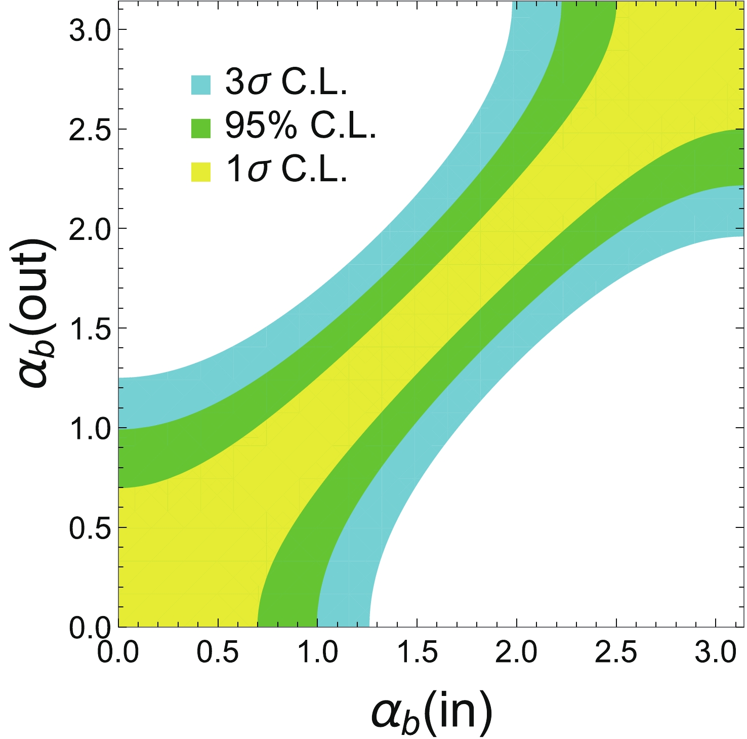
Figure 5. (color online) The
$\alpha_b$ measurement accuracy for the 240 GeV Higgs factory with 5.6 ab−1 integrated luminosity after combining the leptonic and hadronic decaying$Z$ channels;$\alpha_b({{\rm{in}}})$ is the real input of the phase angle, and$\alpha_b({{\rm{out}}})$ is the measured value with uncertainty.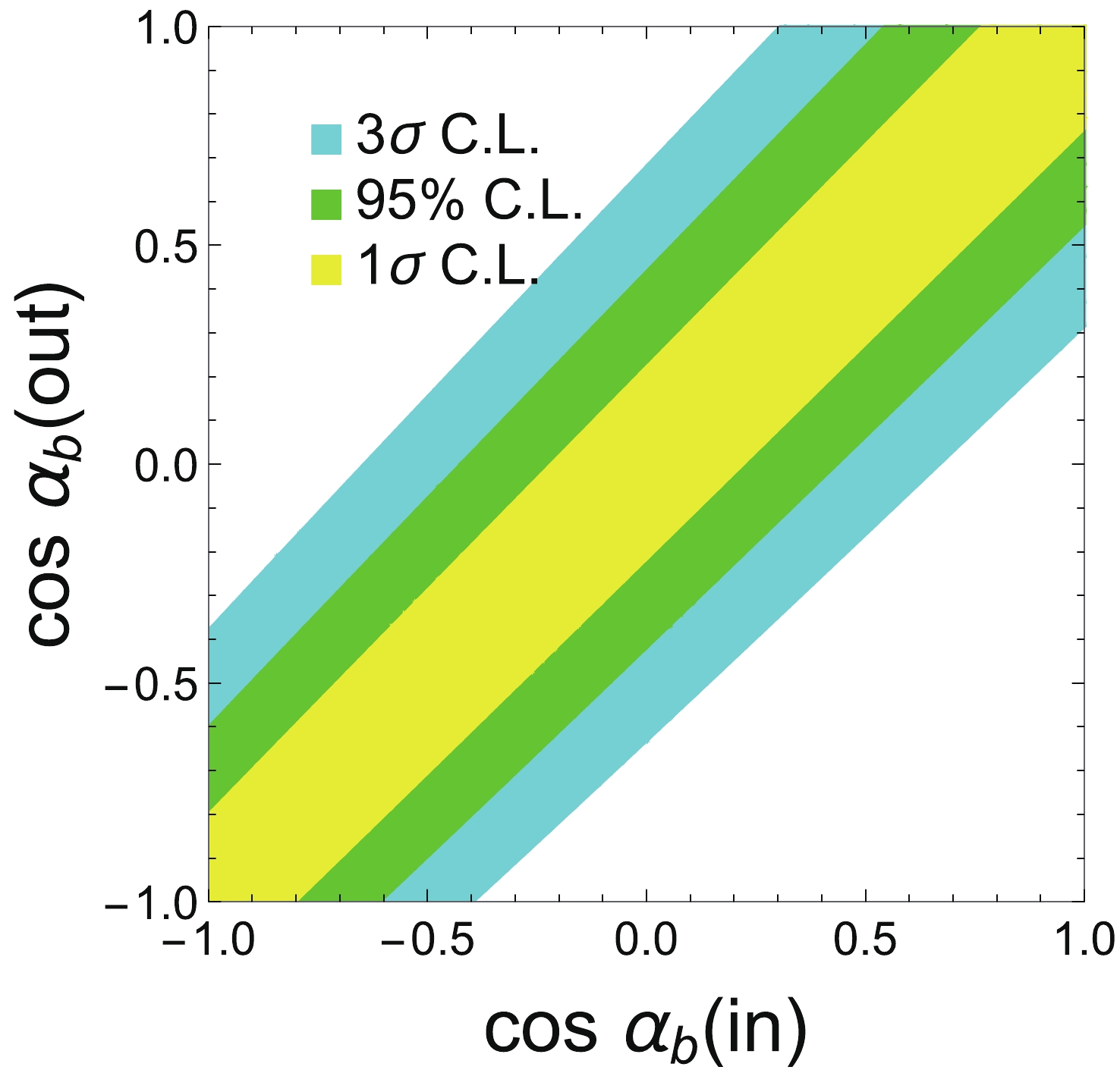
Figure 6. (color online) The
$\cos\alpha_b$ measurement accuracy for the 240 GeV Higgs factory with 5.6 ab−1 integrated luminosity after combining the leptonic and hadronic decaying$Z$ channels;$\cos\alpha_b({{\rm{in}}})$ is the real input of the phase angle, and$\cos\alpha_b({{\rm{out}}})$ is the measured value with uncertainty. -
For the 365GeV
$ e^+e^- $ collider, we generate the events with the same method, choose the smearing parameters and the$ k $ -factor with the same values as those for the 240GeV Higgs factory, and use the same smearing formulas. The kinetic cuts are modified slightly. For the leptonic decaying$ Z $ channel, the$ \theta_{\ell^+\ell^-} $ cut is changed to$ \theta_{\ell^+\ell^-}>60^\circ $ . For the hadronic decaying$ Z $ channel, the likelihood functions of the invariant mass distributions and recoil mass distributions are changed to$ L_Z(m) = P(m;91.1{{\rm{GeV}}},5.58{{\rm{GeV}}}), $

(25) $ L_h(m) = P(m;124.9{{\rm{GeV}}},6.14{{\rm{GeV}}}), $

(26) $ L_{rZ}(m) = P(m;131.88{{\rm{GeV}}},23.84{{\rm{GeV}}}), $

(27) $ L_{rh}(m) = P(m;102.6{{\rm{GeV}}},30.27{{\rm{GeV}}}), $

(28) and the recoil mass distributions do not help us significantly. Finally, we combine the result from the 356 GeV lepton collider with the result from the 240 GeV Higgs factory shown previously. The combined results are shown in Fig. 7, Fig. 8, and Fig. 9.
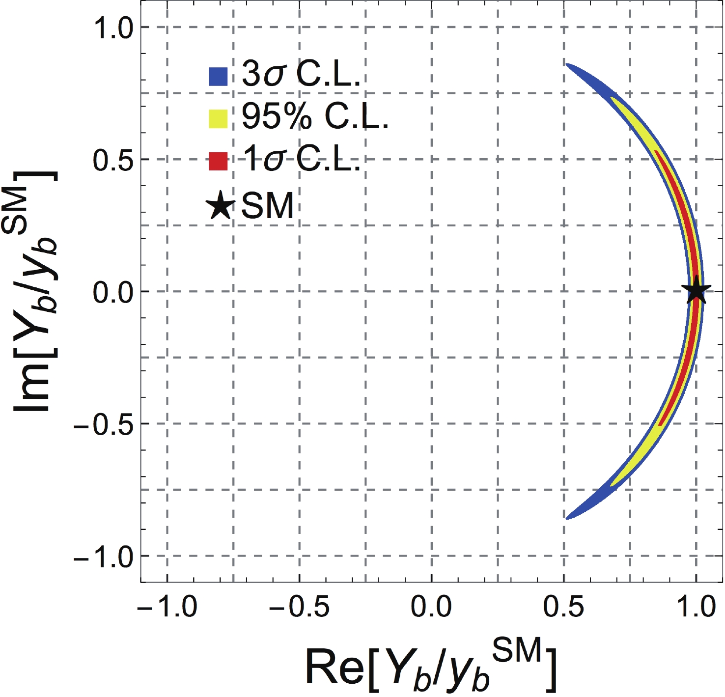
Figure 7. (color online) The constraint of
$Y_b$ for the 240 GeV Higgs factory with 5.6 ab−1 integrated luminosity combined with 365 GeV lepton collider with 1.5ab−1 integrated luminosity after combining the leptonic and hadronic decaying$Z$ channels.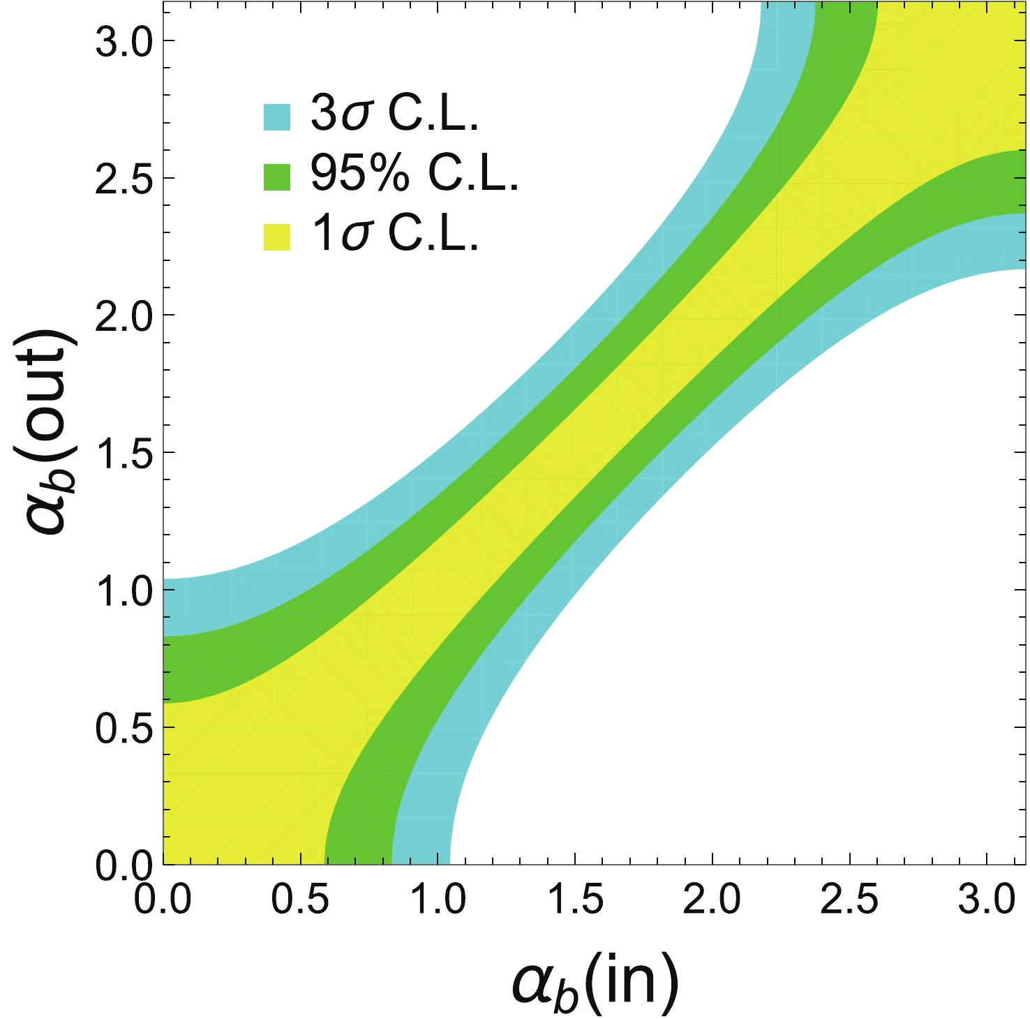
Figure 8. (color online) The
$\alpha_b$ measurement accuracy for the 240 GeV Higgs factory with 5.6 ab−1 integrated luminosity combined with the 365 GeV lepton collider having 1.5 ab−1 integrated luminosity after combining the leptonic and hadronic decaying$Z$ channels;$\alpha_b({{\rm{in}}})$ is the real input of the phase angle, while$\alpha_b({{\rm{out}}})$ is the measured value with uncertainty.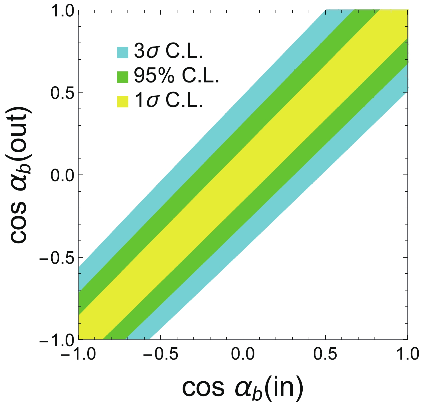
Figure 9. (color online) The
$\cos\alpha_b$ measurement accuracy for the 240 GeV Higgs factory with 5.6 ab−1 integrated luminosity combined with the 365 GeV lepton collider having 1.5 ab−1 integrated luminosity after combining the leptonic and hadronic decaying$Z$ channels;$\cos\alpha_b({{\rm{in}}})$ is the real input of the phase angle, and$\cos\alpha_b({{\rm{out}}})$ is the measured value with uncertainty. -
In this work, we investigate the possibility of measuring the phase angle in the bottom-quark Yukawa interaction for a future Higgs factory. We find that, for a 240 GeV Higgs factory with 5.6 ab−1 integrated luminosity, the accuracy of the measurement could reach
$ \delta(\cos\alpha_b)\sim \pm0.23 $ , which changes a little for different values of$ \cos\alpha_b $ (see Fig. 6). If the Higgs factory runs at 365 GeV and accumulates 1.5 ab−1 integrated luminosity, the accuracy could increase to$ \delta(\cos\alpha_b)\sim \pm0.17 $ (see Fig. 9). This result, combined with the$ hgg $ interaction measurement result from the LHC, can help us fix the phase angle in the bottom-quark Yukawa interaction with the 125 GeV SM-like Higgs boson discovered at the LHC. With such an accuracy of the measurements, NP models with anomalous bottom-quark Yukawa interaction, such as the wrong-sign limit of the type-II 2HDM, will be discovered (or excluded) with a C.L. of at least 3$ \sigma $ .In our simulation, we generated the Monte Carlo events with tree level amplitude. The infra-red (IR) divergence in the cross section is avoided by adding kinematic cuts. There have been a number of studies on the higher order correction to the
$ h{\rightarrow} b\bar b $ decay channel since the 1980s (for example, see [53-66]). Some of these studies include the interference effect with the$ h{\rightarrow} gg $ channel. Because the phase space region that makes the dominant contribution to the measurement is the nearly collinear region of the two$ b $ -jets, a calculation including resummation effects in that region would probably result in a significant improvement in the accuracy of the theoretical prediction.The
$ b $ -tagging efficiency used in this work is high. It is probable that the$ b $ -tagging efficiency at future Higgs factories will not reach the assumed value. There are some potential causes for a decrease in the$ b $ -tagging efficiency. For example, because the two$ b $ -jets are nearly collinear, it may be difficult to tag both of them with high efficiency. Second, the$ b $ -jet in this process is not energetic enough; therefore, the mis-tagging rate of the charm-quark jet could be higher than that of our assumption. However, these will not be severe problems. One may require only one$ b $ -tagged jet in the signal events and accept a higher$ c $ -mis-tagging rate, because the simulation shows that these SM backgrounds are still small enough. When researchers try to analyze the data with a hadronic decay$ Z $ boson, these problems will be more subtle. A more realistic simulation is necessary in this case. Because the hadronic$ Z $ decay branching ratio is much larger, these data may improve the results. Nevertheless, this topic is beyond the scope of our work. -
We thank Edmond L. Berger, Qing-Hong Cao, Lian-Tao Wang, Li Lin Yang, and Jiang-Hao Yu for helpful discussions. HZ would like to thank the staff at Shanghai Jiao-Tong University in Shanghai for their hospitality.
Investigating bottom-quark Yukawa interaction at Higgs factory
- Received Date: 2020-09-16
- Available Online: 2021-02-15
Abstract: Measuring the fermion Yukawa coupling constants is important for understanding the origin of the fermion masses and their relationship with spontaneously electroweak symmetry breaking. In contrast, some new physics (NP) models change the Lorentz structure of the Yukawa interactions between standard model (SM) fermions and the SM-like Higgs boson, even in their decoupling limit. Thus, the precise measurement of the fermion Yukawa interactions is a powerful tool of NP searching in the decoupling limit. In this work, we show the possibility of investigating the Lorentz structure of the bottom-quark Yukawa interaction with the 125 GeV SM-like Higgs boson for future


 DownLoad: