


 Abstract
 HTML
HTML Reference
 Related
 PDF
PDF


-
The China Jinping Underground Laboratory (CJPL), located in Sichuan Province, China, is one of the world's deepest underground laboratories [1]. The rock overburden at CJPL is about 2400 m vertically [2] and the closest nuclear power plant is approximately 1000 km away. It is an ideal site for rare-event experiments such as dark matter searches [3, 4], neutrinoless double beta decay [5, 6], and solar neutrino studies. The proposed Jinping Neutrino Experiment aims to study MeV-scale low-energy neutrinos, including solar neutrinos, geoneutrinos, and supernova relic neutrinos (also referred to as the diffuse supernova neutrino background) [7-9].
These studies are very prone to contamination from cosmic-ray muons and muon-induced radioactive isotope backgrounds. From the dominant vertical muons detected by a plastic scintillator telescope, the first measurement of cosmic-ray flux was
$ (2.0\pm0.4)\times10^{-10} $ cm$ ^{-2} $ s$ ^{-1} $ and had no angular correction to the detector acceptance [10]. Reference [11] categorized underground laboratories into two types: below mountains (mountain shape overburden) and down mine shafts (flat overburden). However, as Ref. [12] pointed out, the flux magnitude is quite different in laboratories situated under mountains and down mine shafts with the same vertical rock overburden. This difference can lead to different background levels for a variety of physics implications, such as the cosmogenic$ ^{11} $ C background in searches for Carbon-Oxygen-Nitrogen solar neutrinos [13], and the cosmic-ray spallation background in searches for the upturn of the solar$ ^{8} $ B neutrino spectrum [14] and supernova relic neutrinos [15]. Therefore, a precise total flux measurement and a detailed cosmic-ray leakage study are necessary for the active and passive shielding design of future neutrino experiments.A 1-ton scintillator detector serves as a prototype of the Jinping Neutrino Experiment and has been running since 2017 [16]. This prototype aims to test the performance of several related key detector components, understand the neutrino detection technology, and measure the underground background level in situ. This study used this omnidirectional detector to measure the cosmic-ray muon flux at CJPL-I, including the muon angular distributions, enabling a clear understanding of the cosmic-ray leakage through the mountain topography profile.
After detailing the design of the 1-ton prototype detector, we describe the model for predicting the underground muon energy and angular distributions, muon event selection, and direction reconstruction. The muon flux measurement based on the two-year data of the 1-ton prototype is then reported.
-
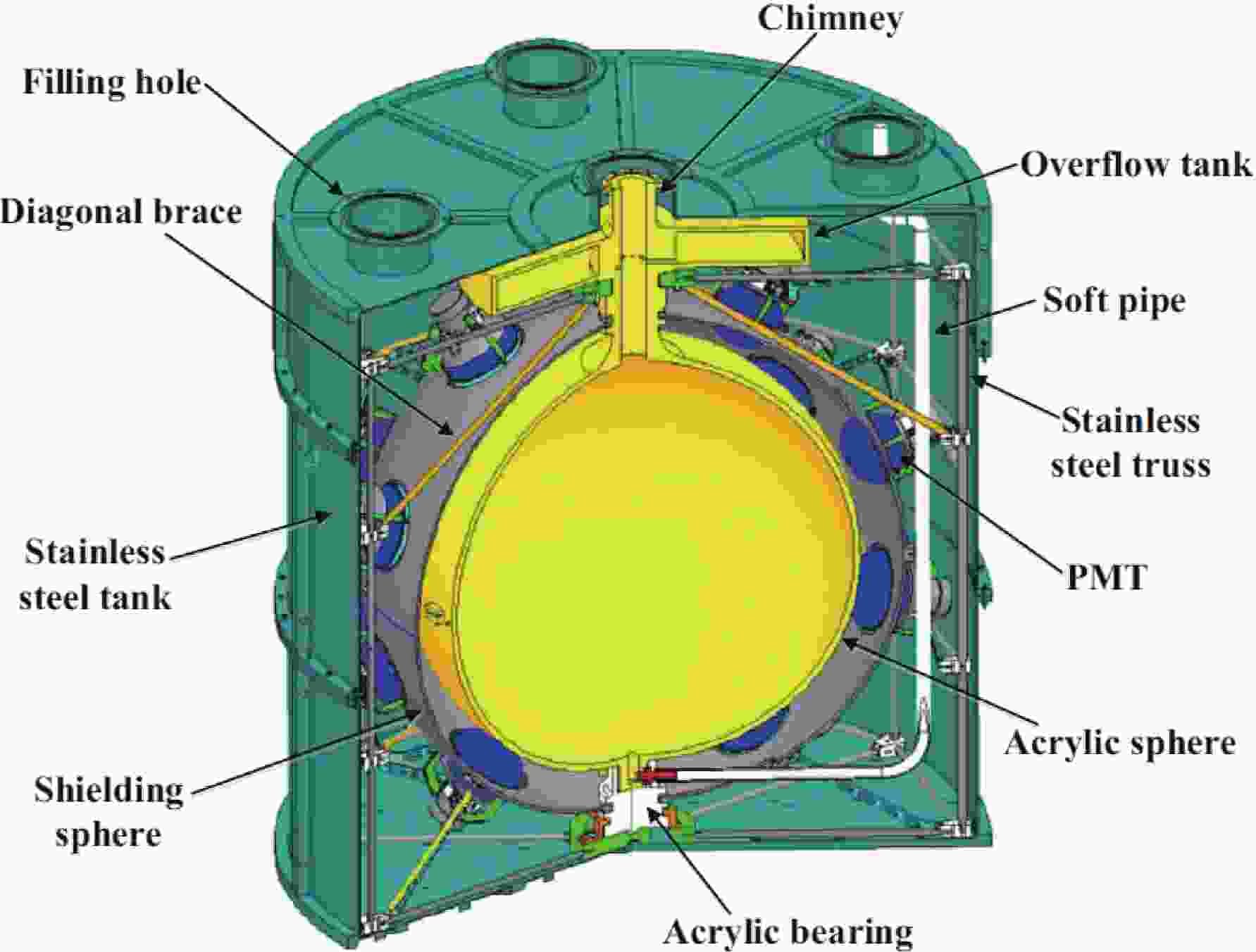
Figure 1 shows a schematic diagram of the detector structure. To reduce the environmental background, 20 cm
$ \times $ 10 cm$ \times $ 5 cm lead bricks were used to form a shielding wall outside the tank (not drawn in the figure). The detector measures 2 m in height and contains one ton of custom liquid scintillator in a 0.645 m-radius acrylic spherical vessel [16]. This scintillator, referred to as the slow liquid scintillator [17, 18], is a linear alkylbenzene (LAB) doped with 0.07 g/l of the fluor 2,5-diphenyloxazole (PPO) and 13 mg/l of the wavelength shifter 1,4-bis (2-methylstyryl)-benzene (bis-MSB). This slow scintillator delays the scintillation light emission duration and thus enhances the Cherenkov-to-scintillation light ratio in the early arrival time, to separate these two lights with high efficacy. Thirty 8-inch Hamamatsu R5912 photomultiplier tubes (PMTs) outside the acrylic vessel detect the Cherenkov and scintillation light and output their pulse shapes to front-end electronics. A water buffer layer between the outer layer of the acrylic vessel and the inner wall of the stainless steel tank serves as a passive shielding material to suppress the ambient radioactive background.
Figure 1. (color online) 1-ton prototype of Jinping Neutrino Experiment.
The front-end electronics system includes 4 CAEN V1751 FlashADC boards and one logical trigger module CAEN V1495. Each FlashADC board has eight channels, with 10 bit ADC precision for 1 V dynamic range, and a 1 GHz sampling rate. All the PMT signals go directly into the V1751 boards for digitization. If more than 25 PMTs fired, the data acquisition system records all the pulse shapes from the fired PMTs in a 1029-ns time window.
-
The energy spectrum and angular distribution of underground muons were used as the inputs for the detector simulation. The muon direction is defined throughout this paper as the direction from which it comes. A Geant4 [19, 20]-based package simulated muon penetration development in the mountain rock to predict various underground muon characteristic profiles, with its own standard electromagnetic and muon-nucleus processes.
Jinping mountain is about 4000 m above sea level, and the elevation of the experiment hall is about 1600 m. We obtained the mountain terrain data from the NASA SRTM3 dataset [21]. Figure 2 shows the contour map. There were 6315 survey points within a 9 km radius circle centered at the laboratory. We assembled them to a mesh using Delaunay triangulation, a standard algorithm, to divide discrete points into a set of triangles with the restriction that two adjacent triangles entirely share each triangle side.
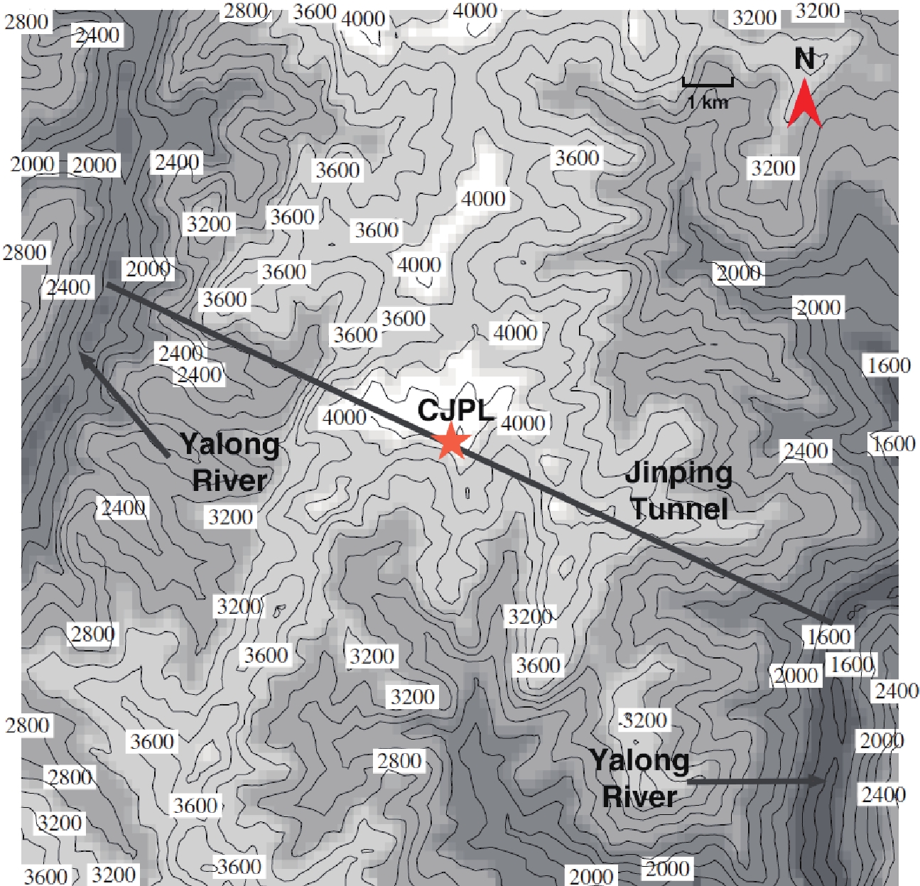
Figure 2. (color online) Contour map near CJPL-I, as given by the SRTM3 dataset [21].
We assume Jinping mountain's average rock density to be 2.8 g/cm
$ ^3 $ , from Ref. [10], so the water equivalent depth is 6720 m for 2400 m rock. The density variation can affect the simulated spectrum. However, it is negligible for the flux measurement since, in our case, the detection efficiency is not sensitive to the spectrum, as discussed in Sec. VI.C. The composition of the rock in the simulation utilized the values from the abundance of elements in Earth’s crust (percentage by weight) [22]: oxygen (46.1%), silicon (28.2%), aluminum (8.2%), and iron (5.6%). The modified Gaisser’s formula [23] parametrizes the kinetic energy E and zenith angle$ \theta $ distribution of cosmic-ray muons at sea level as$ \begin{aligned}[b]G(E,\theta)\equiv &\frac{ {\rm{d}} N}{ {\rm{d}} E {\rm{d}} \Omega} = \frac{I_0}{{\rm{cm}}^2\cdot {\rm{s}}\cdot {\rm{sr}}\cdot{\rm{GeV}}}\\&\times \left(\frac{E^{\star}}{{\rm{GeV}}}\right)^{-\gamma}\cdot \left(\frac{1}{1+\dfrac{1.1E\cos\theta^\star}{115\;{\rm{GeV}}}}+\frac{0.054}{1+\dfrac{1.1E\cos\theta^\star}{850\;{\rm{GeV}}}}\right), \end{aligned} $

(1) where
$ E^\star $ and$ \cos\theta^\star $ are defined as follows:$ \begin{aligned}[b] E^{\star} =& E\left[1+\frac{3.64\,{\rm{GeV}}}{E\cdot(\cos\theta^\star)^{1.29}}\right], \\ \cos\theta^\star =& \sqrt{\frac{\cos^2\theta+P_1^2+P_2(\cos\theta)^{P_3}+P_4(\cos\theta)^{P_5}}{1+P_1^2+P_2+P_4}} , \end{aligned}$

(2) where
$ I_0 $ is a normalization constant,$ \gamma = 2.7 $ is the muon spectral index, and$ P_1,P_2,P_3,P_4 $ , and$ P_5 $ are the parameters in Ref. [23].Figures 3 and 4 show the simulated underground muon kinetic energy and corresponding angular distributions at CJPL-I. The uncertainties come from the precision of the NASA dataset (90 m in horizon directions) and the experiment hall size of
$ \sim100 $ m. We also plot the distributions at sea-level for comparison. The expected corresponding zenith angle follows a$ \cos^2\theta $ distribution and the azimuth angle follows a uniform distribution. The observed cosmic-ray leak in the southern direction agrees with Fig. 2, in which the contour plot indicates less rock coverage.
Figure 3. (color online) Simulation result of underground muon kinetic energy. The mean value is 340 GeV. The gray band shows the 1
$\sigma$ uncertainty. See more details in the text. The spectrum of muons at sea-level is also plotted.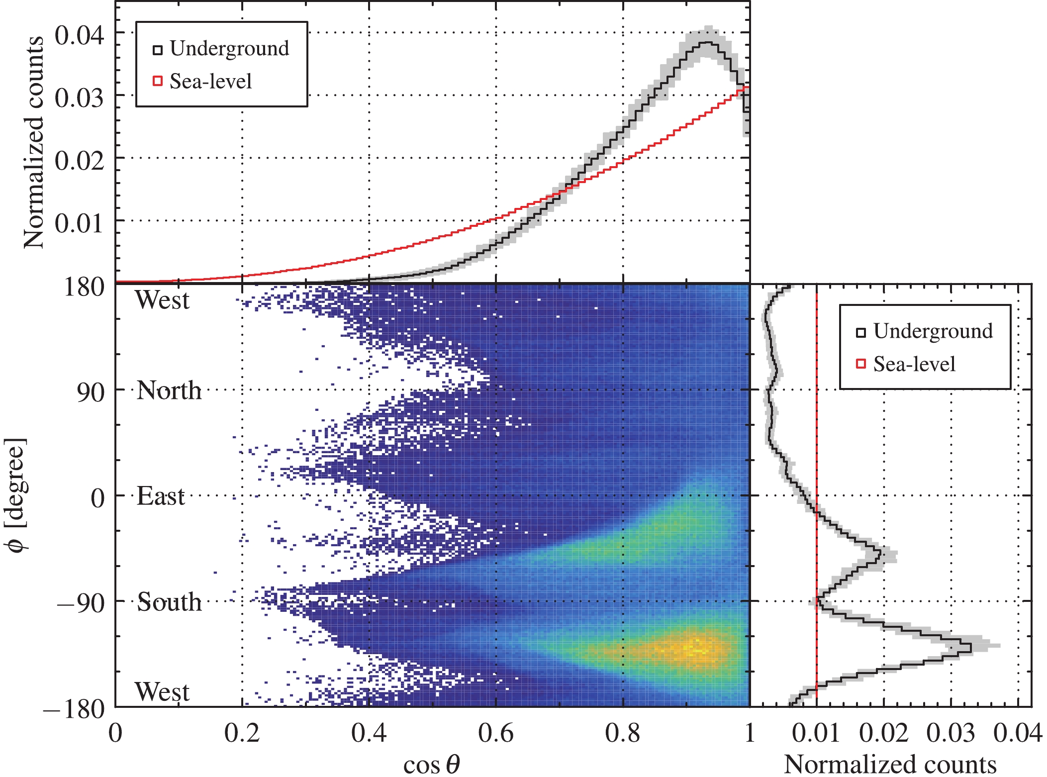
Figure 4. (color online) Simulation result of underground muon direction
$(\cos\theta,\phi)$ and one-dimensional projections. Muons from the south are more intense, as expected from the contour map in Fig. 2. The gray band shows the 1$\sigma$ uncertainty. See more details in the text. The spectrum of muons at sea-level is also plotted.Due to the high elevation (
$ \sim $ 4000 m), the altitude and latitude may affect the muon distributions described in Eq. (1). However, Ref. [24] pointed out that the differential flux at high energy ($ >40 $ GeV) and small zenith angle barely depends on altitude and latitude. Since the minimum energy required for muons to reach CJPL-I is approximately 3 TeV, and the cosine of the zenith angle is concentrated above 0.4, we conclude that CJPL-I's altitude and latitude do not affect the underground muon spectrum. -
This study analyzed the data collected from July 31, 2017 to July 12, 2019. We first required that runs should be flagged as good runs, i.e., neither pedestal calibration nor detector maintenance. Data quality check parameters for identifying apparent noise were the trigger rate, baseline, and baseline fluctuation of a waveform. A data file should not have these quantities deviate from the reference values by more than three standard deviations. The live time after the data quality check was
$ 5.575\times10^7 $ s, or 645.2 live days.We then required a minimum number of photoelectrons (PEs), corresponding to approximately 100 MeV energy deposits or 50 cm track length in the scintillator. When passing through the detector's edge, a muon deposits less energy and is indistinguishable from that from the radioactive background, muon showers, or noise events. Therefore, this cut discarded low-energy events to get a high purity sample.
We finally removed the electronics noise and flasher events, which are highly-charged light-emitting events, possibly from discharge of the PMT bases. Examining all the high energy deposit event waveforms, we found that some of them always had a single PMT with a much higher charge than the others, while a muon event was of a more uniform charge distribution. To identify the flasher events, we required that the ratio of maximum PE number of each PMT to total PE number in one event, denoted by
$ r_{\rm{max}} $ , should not be greater than 0.15 to identify the flasher events.Figure 5 shows a two-dimensional distribution and one-dimensional projections of PE number and
$ r_{\rm{max}} $ , indicating that the flasher events and the electronic noise events correspond to the clusters with larger$ r_{\rm{max}} $ . We also show the simulation result and one-dimensional projections for better comparison. In the end, 264 muon candidates passed the selection criteria. Table 1 summarizes all the selection criteria for muon candidate selection.Type Selection criteria Data quality check Good run Trigger rate, baseline and baseline fluctuation Muon candidate selection Number of photoelectrons $>6000$ 

$r_{\rm{max}}<0.15$ 

Table 1. Summary of cuts for muon candidate selection.
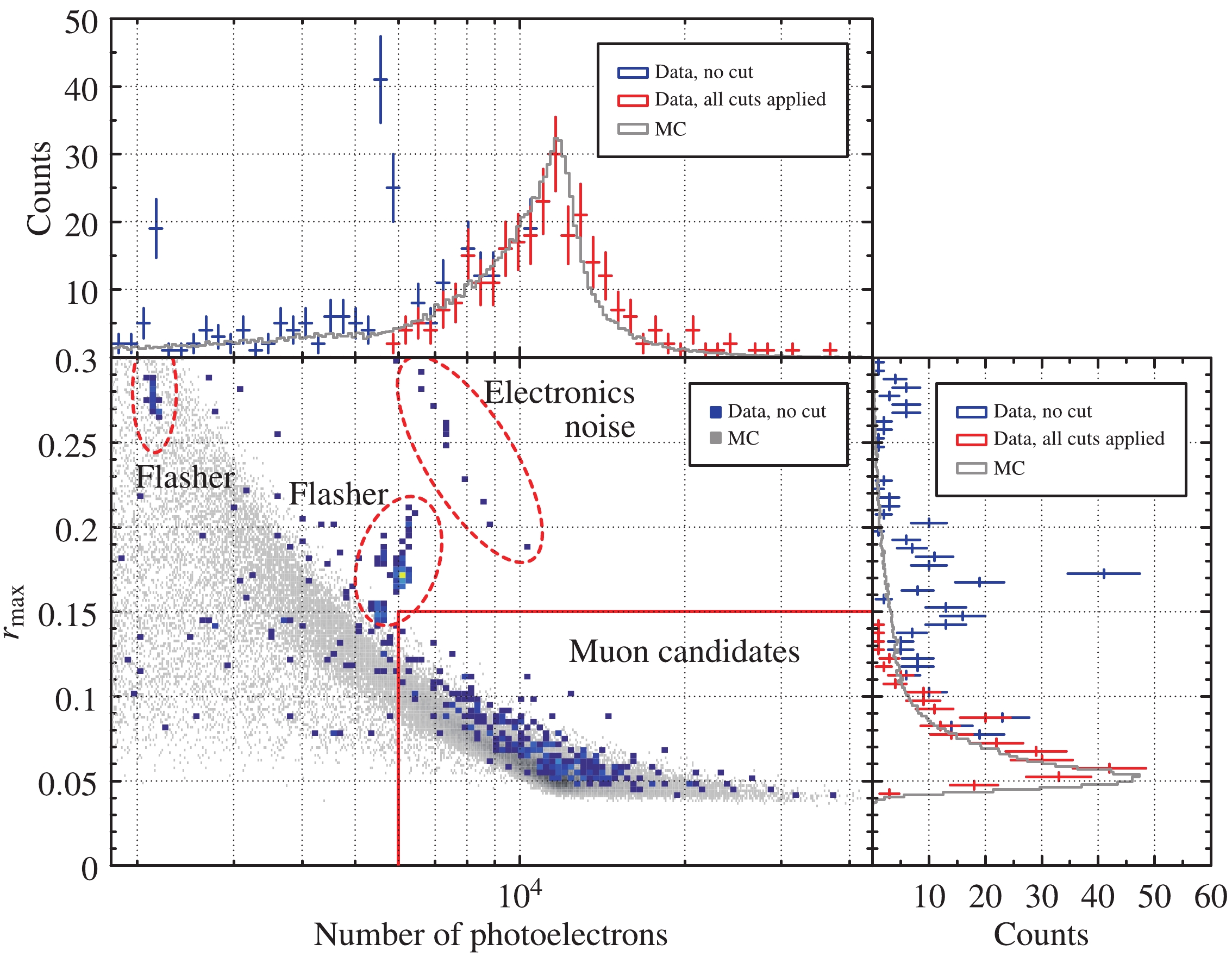
Figure 5. (color online) Scatter plot and one-dimensional projections of
$r_{\rm{max}}$ and PE number distribution from the data. The grey area in the two-dimensional distribution is the simulation result. Typical muon candidates spread in the region of$r_{\rm{max}}<0.15$ and PE number$>6000$ , while flasher and electronics noise events have larger$r_{\rm{max}}$ and are distributed in the clusters marked with circles. Low-energy events (PE number$<6000$ ) which may contain indistinguishable radioactive background, shower, or noise events are also removed. -
We used a template-based method to reconstruct the muon direction. The templates were generated from a Geant4-based simulation. Each template was tagged with the muon direction
${{p}}_i = (\cos\theta,\phi)$ and the entry point on the acrylic vessel$ (\cos\alpha,\beta) $ , as shown in Fig. 6. When a muon's direction was sampled from a uniform distribution, its entry point on the vessel surface was also sampled uniformly on the hemisphere facing the muon direction.
Figure 6. (color online) Muon generator in the PMT trigger time pattern template. The muon direction
$(\cos\theta,\phi)$ and entry point$(\cos\alpha,\beta)$ were sampled uniformly.About 250k template events passed the event selection criteria described in Section 4. For the PMT arrival time pattern vector of template i:
${{T}}_i = (t_{0i},t_{1i},\cdots,t_{29i})$ , we subtracted the mean value$ \bar{t}_i = \dfrac{1}{30}\displaystyle\sum^{29}_{j = 0}t_{ji} $ for zero centering,$ \tilde{{{T}}}_i = (\tilde{t}_{0i},\tilde{t}_{1i},\cdots,\tilde{t}_{29i}) = (t_{0i}-\bar{t}_i,t_{1i}-\bar{t}_i,\cdots,t_{29i}-\bar{t}_i) . $

(3) The zero-centered PMT arrival time pattern vector for data is
$ \tilde{{{T}}} = (\tilde{t}_{0},\tilde{t}_{1},\cdots,\tilde{t}_{29}) = (t_{0}-\bar{t},t_{1}-\bar{t},\cdots,t_{29}-\bar{t}), $

(4) where
$ \bar{t} = \dfrac{1}{30}\displaystyle\sum^{29}_{j = 0}t_{j} $ . We constructed the corresponding Euclidean distance,$ d_i = \lvert\tilde{{{T}}}_i-\tilde{{{T}}}\rvert = \sqrt{\sum\limits_{j = 0}^{29}\left(\tilde{t}_{ji}-\tilde{t}_{j}\right)^2} \ . $

(5) Then we searched for the k nearest neighbors, where the hyper-parameter k is an arbitrary integer to be chosen later. The reconstructed muon direction
${{P}}$ was calculated by the weighted average of the k nearest neighbors,$ {{P}} = \dfrac{\displaystyle\sum_{i = 1}^k\dfrac{1}{d_i}{{p}}_i}{\displaystyle\sum_{i = 1}^k\dfrac{1}{d_i}}\ . $

(6) We generated a test sample (also uniform muons) to evaluate the reconstruction method performance and determine the hyper-parameter k. The smearing induced by the detector response was included in the test sample to simulate the uncertainty from the electronics hardware and the time calibration. Figure 7 shows that the average included angle between the truth and the reconstructed directions
$ \Delta\Theta $ varies with the hyper-parameter k and becomes stable at$ k = 50 $ and above. Therefore, we chose$ k = 50 $ for the reconstruction. Figure 8 shows that the included angle distribution has a peak value of 10 degrees and an average of 20 degrees. The long tail is due to the limited time resolution of the electronics hardware and PMTs.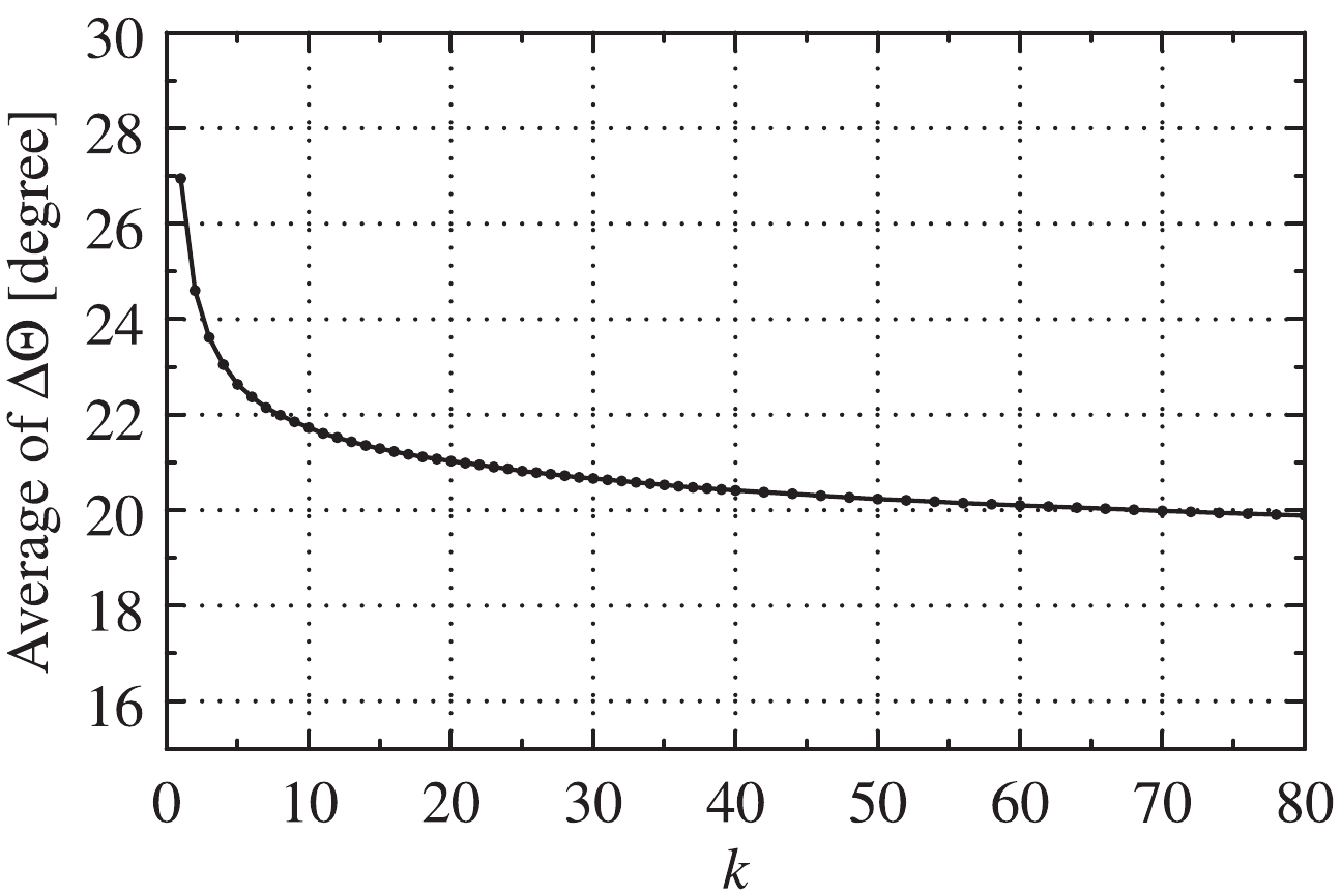
Figure 7. Average included angle
$\Delta\Theta$ between the truth and reconstructed directions as a function of the hyper-parameter k.
Figure 8. Included angle
$\Delta\Theta$ between the truth and the reconstructed directions for$k=50$ .Figure 9 shows the
$ \cos\theta $ and$ \phi $ distributions for both the data and the simulation. Both are consistent. The uneven structure observed for the$ \phi $ distribution indicates the different cosmic-ray leakage due to the mountain structure above CJPL-I.
Figure 9. (color online) Reconstructed
$\cos\theta$ and$\phi$ for the selected muon candidates. Also plotted are the one-dimensional projections for these two angles for the data (black) and the simulation (red). -
We define the overall efficiency
$ \epsilon $ as the ratio of the number of selected muon candidates$ N_\mu $ over the total number of muons going through the experiment hall$ N_{\rm{total}} $ ,$ \epsilon\equiv\frac{N_{\mu}}{N_{\rm{total}}}. $

(7) The selected muon candidates contain a small fraction of the muon shower events, due to muon interactions with the atoms of the rock. As a consequence, the incident particles are the parent muons. We had to evaluate this effect in the detection efficiency, so we simulated the whole experiment hall. With the underground muon energy spectrum and angular distribution in Section III, we performed another Geant4-based simulation to study the detection efficiency. Considering the effect of muon showers in the rock and detector components, we added 1 m thick rock in the geometry and generated muons flying towards the five surfaces (excluding the bottom surface) of an 8 m
$ \times $ 6 m$ \times $ 5 m experiment hall, as shown in Fig. 10.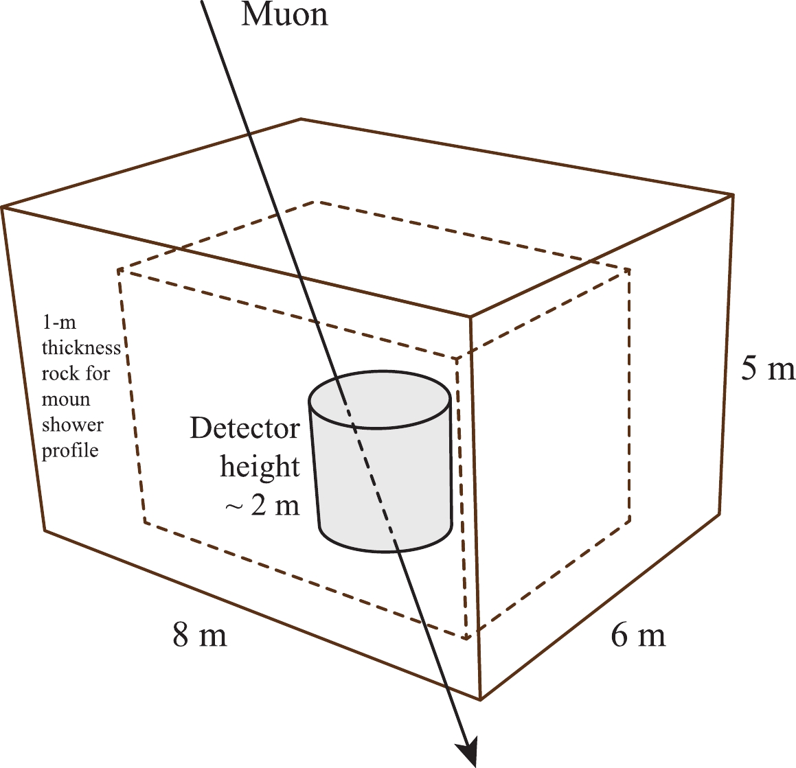
Figure 10. Geometry setup in the simulation.
After being decomposed into a geometry factor
$ \epsilon_g $ , a detection efficiency$ \epsilon_d $ , and a shower factor$ \epsilon_s $ , the overall efficiency becomes$ \epsilon = \epsilon_g\cdot\epsilon_d+\epsilon_s, $

(8) $ \epsilon_g = \frac{N_p}{N_{\rm{total}}},\quad\epsilon_d = \frac{N_1}{N_p},\quad \epsilon_s = \frac{N_2}{N_{\rm{total}}}, $

(9) where
$ N_p $ is the number of muons passing through the scintillator target,$ N_1 $ is the number of detected muons passing through the scintillator target, and$ N_2 $ is the number of detected muon shower events,$ N_\mu = N_1+N_2 $ . The simulation results show that$ \epsilon = 1.70\%,~\epsilon_g = 2.02\%,~\epsilon_d = 82.7\%,~\epsilon_s = 0.04\%. $

(10) The detection efficiency
$ \epsilon_d = $ 82.7% indicates that the efficiency loss in the event selection is less than 20%.As shown in Fig. 11, for a surface S with normal direction
$ (\alpha_{\rm{zenith}},\beta_{\rm{azimuth}}) $ and muon direction$ (\theta, \phi) $ , the horizontal projection area$ S_{\rm{p}} $ is given by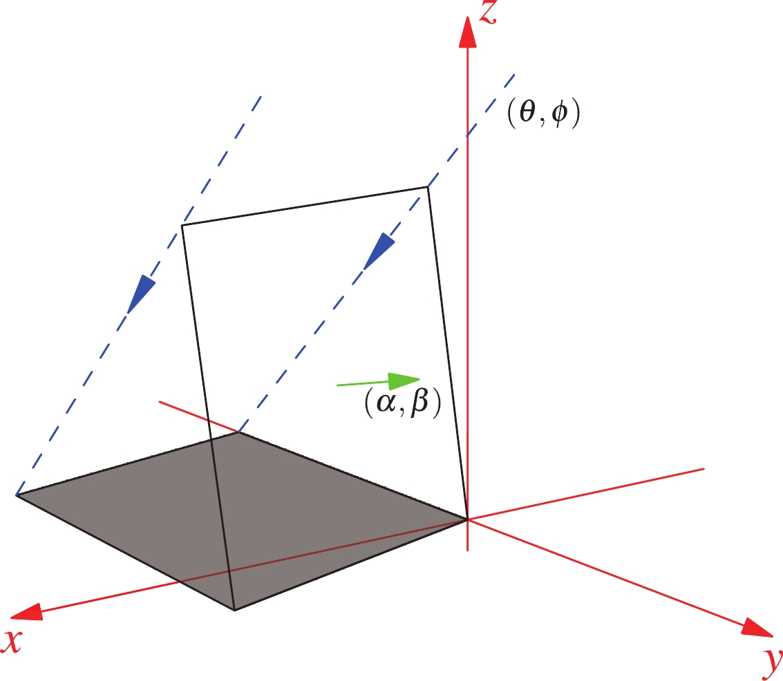
Figure 11. (color online) Projection area (gray) of the surface
$(\alpha,\beta)$ for the muon direction$(\theta,\phi)$ .$ S_{\rm{p}}(\theta, \phi) = \left|\sin \alpha \tan \theta \cos (\beta -\phi )+\cos \alpha \right|S . $

(11) We define
$ S_{i} $ as the projection area of the i-th surface, which is an integral for the normalized incoming muon spectrum$ f(E_k, \theta,\phi) $ obtained from the simulation result of Section III,$ S_i = \int S_{{\rm{p}}}(\theta, \phi) f(E_k, \theta,\phi)\,{\rm{d}}(\cos\theta){\rm{d}}\phi . $

(12) The experiment hall projection area
$ S_{\rm{total}} $ is the sum of the five surfaces,$ S_{\rm{total}} = \sum\limits_{i = 1}^5S_i = 78.7\, \rm{m}^2. $

(13) -
The muon flux
$ \phi_\mu $ was calculated by$ \phi_\mu = \frac{N_{\rm{total}}}{T\cdot S_{\rm{total}}} = \frac{N_\mu/\epsilon}{T\cdot S_{\rm{total}}}, $

(14) where T is the live time and
$ N_\mu $ is the number of muon candidates. By defining$ S\equiv\epsilon S_{\rm{total}} $ as the active area, we simplified the 1-ton prototype detector flux calculation to$ \phi_\mu = \frac{N_\mu}{T\cdot S} = 3.53\times10^{-10}\,{\rm{cm}}^{-2}{\rm{s}}^{-1} . $

(15) The simulation results show that the active area
$ S = 1.34 $ m$ ^2 $ is close to the cross-section of the liquid scintillator sphere of the detector, which is 1.31 m$ ^2 $ . -
Table 2 summarizes the systematic uncertainties, which mainly come from two components: (1) the PE number calculation (energy scale) in the data and (2) the efficiency calculation in the Monte-Carlo simulation. A quadrature sum of the individual components gives the total systematic uncertainty.
Source Parameter uncertainty Flux measurement uncertainty Energy scale $\pm2.0$ %

$\pm0.6$ %

Efficiency calculation PE yield $\pm1.6$ %

$\pm0.5$ %

Acrylic vessel radius $\pm0.5$ cm

$\pm1.6$ %

Lead shielding thickness $\pm5$ cm

±0.6%* Rock thickness for muon shower profile $\pm50$ cm

±0.8%* Muon spectra − ±0.7%* Total systematic − $\pm2.2$ %

Statistical − $\pm6.2$ %

$^*$ Dominated by the statistical uncertainty of the Monte Carlo process.

Table 2. Summary of uncertainties for the muon flux measurement.
The conversion from the charge to the number of PEs was done through a PMT gain factor. A run-by-run PMT calibration corrected the gain drift and introduced a 2.0% systematic uncertainty for the 6,000 p.e. cut, corresponding to a 0.6% efficiency variation in flux measurement.
The uncertainty in the efficiency calculation comes from the parameters in the simulation inputs. We compared the data and simulation PE distribution and tuned the scintillation light yield to ensure consistency between the data and simulation. The systematic uncertainty for the consistency was obtained from the Pearson's
$ \chi^2 $ ,$ \chi^2 = \sum\limits_{i = 1}^{\rm{nbins}}\frac{(n_{i}^{\rm{data}}-n_{i}^{\rm{sim}})^2}{n_i^{\rm{data}}} , $

(16) where
$ n_{i}^{\rm{data}} $ is the count in the i-th bin for the data distribution, and$ n_i^{\rm{sim}} $ is the count in the i-th bin for the simulation distribution. The systematic uncertainty of PE yield in the simulation was set to the variation at$ \chi^2_{\min}+1 $ .The acrylic vessel is formed of two hemispheres glued together, for which the machining accuracy was estimated to 5 mm according to the international tolerance grade. This contributed a 1.6% systematic uncertainty in the efficiency calculation.
The muon showers in the rock and lead shielding also contributed to the global efficiency. We placed 1 m depth of rock in the simulation. To verify whether that depth is enough, we added or subtracted 0.5 m rock in different simulations to observe the variation and found that the global efficiency was not sensitive to rock depth. The lead wall thickness was not uniform due to different arrangements of the lead bricks. We changed the thickness by
$ \pm5 $ cm, the typical size of a lead brick, in the simulations, and found little variation in the global efficiency. Limited by the statistical uncertainty of Monte-Carlo, the above studies gave 0.6% and 0.8% systematic uncertainty for the muon shower effect.We scanned different muon spectra (energy and angular distribution) in Section III in the detection efficiency simulation. Thanks to the detector's spherical symmetry, the uncertainty from the muon spectra was also small and dominated by the statistical uncertainty of the Monte Carlo process.
-
The monthly average muon candidate rate appears constant in Fig. 12. The seasonal modulation of muon flux is unobservable because the statistical uncertainty is much larger than the seasonal variation (
$ \sim1.3 $ % in Ref. [25]). The total measured cosmic-ray muon flux is$ (3.53\pm0.22_{\rm{stat.}}\pm0.07_{\rm{sys.}})\times10^{-10} $ cm$ ^{-2} $ s$ ^{-1} $ . The vertical intensity I is calculated to be$ (2.0\pm0.3_{\rm{stat.}})\times10^{-10} $ cm$ ^{-2} $ s$ ^{-1} $ sr$ ^{-1} $ using the 47 muon candidates ($ N_I $ ) reconstructed in$ 0.95<\cos\theta<1 $ ,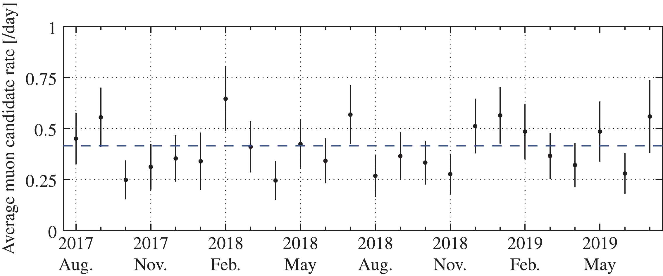
Figure 12. (color online) Cosmic-ray muon rate measured by the 1-ton prototype at CJPL-I, as a function of time. The data are shown in monthly bins.
$ I = \frac{N_I}{T\cdot S\cdot\Omega}, $

(17) where T and S are the live time and active area described in Sec. VI.B, and
$ \Omega = 0.314 $ is the solid angle for$ 0.95<\cos\theta<1 $ . We also studied the flux variation as a function of horizontal location at CJPL-I using a Geant4-based simulation. The result indicated that the variation should be less than 2.3% along the east-west direction within a variation of 100 m.Figure 13(a) shows the vertical intensity of muons at WIPP [26], Soudan [27], Boulby [28], Sudbury [29], Kamioka [30], Gran Sasso [25], Fréjus [31], and Jinping as a function of vertical overburden. Also plotted is the prediction by a parametrized formula, given by Ref. [12],
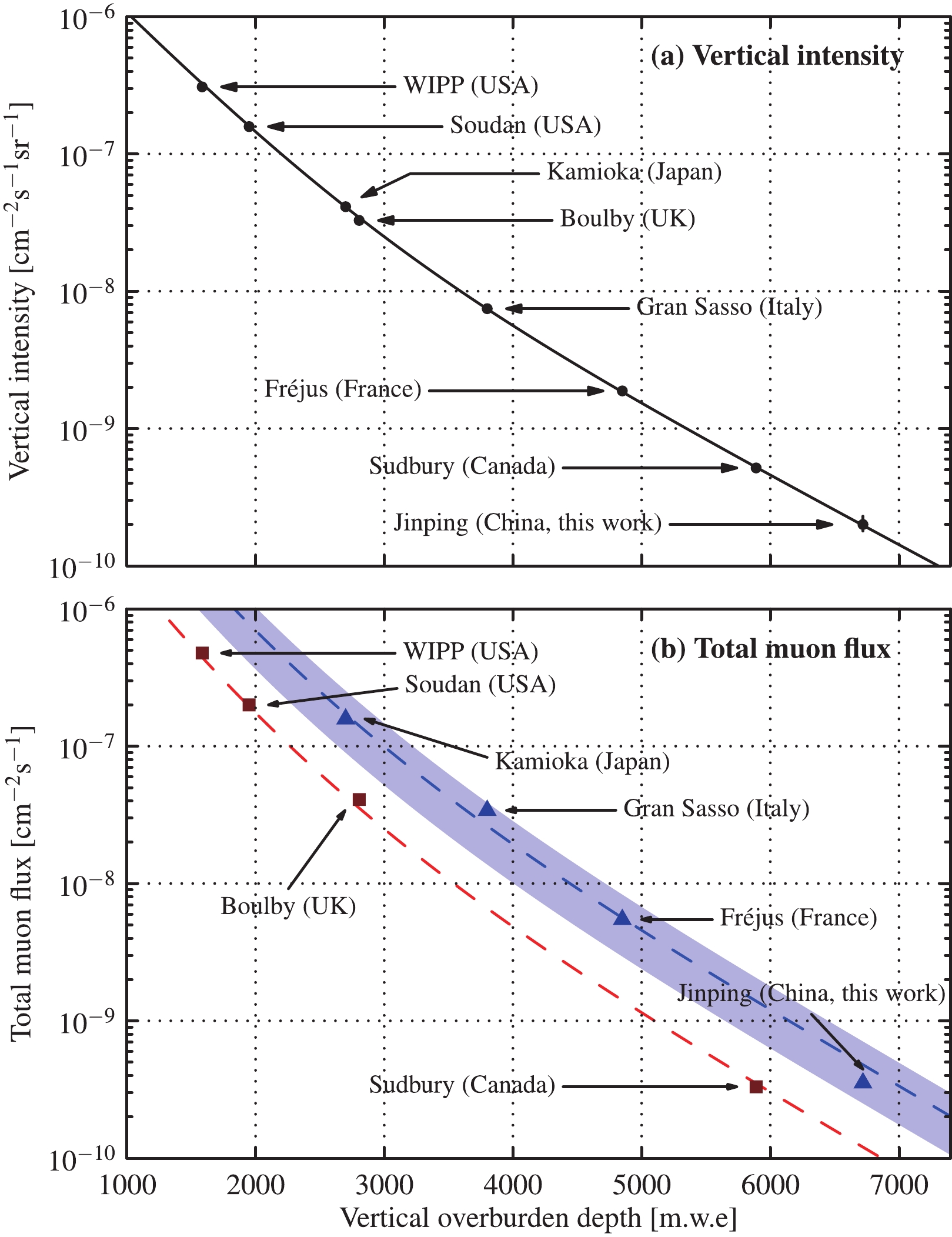
Figure 13. (color online) Measurements of the vertical intensity (a) and total muon flux (b) at different underground sites. The red dashed line in (b) is the empirical formula for the mine shaft case. The blue dashed line and shaded area in (b) are the fitting result and uncertainty respectively for the factor F.
$ I(h) = I_1 {\rm{e}}^{-h/\lambda_1}+I_2 {\rm{e}}^{-h/\lambda_2} $

(18) where
$ I(h) $ is the differential muon intensity corresponding to the slant depth h, and$ I_1, I_2, \lambda_1, \lambda_2 $ are parameters in Ref. [12]. The measurement result in this work is consistent with Eq. (18).Figure 13(b) summarizes the total muon flux measured at different underground sites. WIPP, Soudan, Boulby, and Sudbury are labs situated down mine shafts, while Kamioka, Gran Sasso, Fréjus, and Jinping are below mountains. The underground muon flux
$ \phi $ is a complicated integral over the muon spectrum$ f(E_k,\theta,\phi) $ and slant depth (or muon track length) d,$ \phi = \int f(E_k,\theta,\phi)\cdot p(E_k,d)\, {\rm{d}} E_k {\rm{d}}\theta {\rm{d}}\phi , $

(19) where
$ p(E_k,d) $ is the survival probability at slant depth d. For the mine shaft (flat overburden) case, we have$ d = h/\cos\theta $ . We simulated the muon flux at 50 different depths for the flat overburden case, using Geant4. For simplicity, we fitted these simulation points with a series expansion of Eq. (19),$ \phi_0(h) = \exp\left(a_0+a_1h+a_2h^2+a_3h^3+a_4h^4\right)\,{\rm{cm}}^{-2}{\rm{s}}^{-1} , $

(20) where
$ \phi_0(h) $ is the muon flux at vertical overburden depths h (in km.w.e),$ a_0 = -10.147 $ ,$ a_1 = -3.385\,{\rm{km}}^{-1} $ ,$ a_2 = 0.404\,{\rm{km}}^{-2} $ ,$ a_3 = -0.0344\,{\rm{km}}^{-3} $ ,$ a_4 = 0.00111\,{\rm{km}}^{-4} $ . The differences between the empirical formula and data are$ -6.9 $ % (WIPP),$ -2.6 $ % (Soudan),$ -13.3 $ % (Boulby), and$ 5.7 $ % (Sudbury). The red dashed line in Fig. 13(b) plots the fitting result.The total muon flux of a lab situated below a mountain,
$ \phi_1(h) $ , can be scaled by a factor F to$ \phi_0(h) $ ,$ \phi_1(h) = F\cdot\phi_0(h). $

(21) Usually
$ F>1 $ because the mountain case has less rock shielding, which leads to a more considerable muon flux. The factors F were 3.7 (Kamioka), 5.2 (Gran Sasso), 3.9 (Fréjus) and 2.9 (Jinping). We assumed that mountains on the Earth have similar topography and elemental compositions so that the factors for different locations would not vary too much. We fitted these four labs using the empirical formula in Eq. (21) with an uncertainty assigned so that$ \chi^2/ $ ndf is one. The fitting result$ F = (4.0\pm1.9) $ and this uncertainty account for the variation of mountain topography profiles. The blue dashed line in Fig. 13(b) illustrates the fitting result. Using$ \phi_0 $ and factor F, anyone can easily get a rough estimate from the vertical overburden without doing any simulation or measurement. -
We studied the cosmic-ray muons at CJPL-I using the 1-ton prototype of the Jinping Neutrino Experiment. This study determined the muon flux to be
$ (3.53\pm0.22_{\rm{stat.}}\pm 0.07_{\rm{sys.}})\times10^{-10} $ cm$ ^{-2} $ s$ ^{-1} $ . The zenith and azimuth angle distributions show that cosmic-ray leakage is due to the mountain topography profile, as expected. A survey of muon fluxes at different laboratories situated under mountains and down mine shafts indicated that the flux at the former is generally a factor of$ (4.0\pm1.9) $ larger than at the latter, for the same vertical overburden. This study provides a reference for passive and active shielding designs for future underground neutrino experiments. -
We acknowledge Orrin Science Technology, Jingyifan Co., Ltd, and Donchamp Acrylic Co., Ltd, for their efforts in the engineering design and fabrication of the stainless steel and acrylic vessels. Many thanks to the CJPL administration and the Yalong River Hydropower Development Co., Ltd. for logistics and support.
Muon flux measurement at China Jinping Underground Laboratory
- Received Date: 2020-07-31
- Accepted Date: 2020-09-30
- Available Online: 2021-02-15
Abstract: China Jinping Underground Laboratory (CJPL) is ideal for studying solar, geo-, and supernova neutrinos. A precise measurement of the cosmic-ray background is essential in proceeding with R&D research for these MeV-scale neutrino experiments. Using a 1-ton prototype detector for the Jinping Neutrino Experiment (JNE), we detected 264 high-energy muon events from a 645.2-day dataset from the first phase of CJPL (CJPL-I), reconstructed their directions, and measured the cosmic-ray muon flux to be


 DownLoad: