


 Abstract
 HTML
HTML Reference
 Related
 PDF
PDF


-
Although ground-state hyperons were discovered more than 60 years ago and have played a key role in our understanding of the weak interaction, there are still open questions concerning their weak decay mechanisms. In particular, the hyperon weak radiative decays provide a unique probe for studying the weak, strong, and electromagnetic (EM) interactions [1]. This process generally has a very small branching ratio and is difficult to measure. Recently, BESIII has collected more than 1 billion
$ J/\psi $ events, which can provide a golden opportunity to investigate the properties of the hyperons produced in$ J/\psi $ decays. In particular, it is time to revisit the detailed dynamics of the hyperon weak radiative decays.One of the long-standing questions associated with the hyperon weak radiative decays is the so-called “Hara theorem” [2]. It was shown in Ref. [2] that the parity-violating amplitudes for
$ \Sigma^+ \to p \gamma $ and$ \Xi^- \to \Sigma^- \gamma $ are zero in the limit of unitary symmetry within the pole approximation [3]. However, experimental measurements did not support this prediction, and the asymmetry parameter was found to be large for$ \Sigma^+ \!\to\! p \gamma $ , with a negative sign [4].There is an abundant amount of literature regarding theoretical efforts to understand the physics behind the Hara theorem and the experimental observations. A unified theory was proposed by Zenczykowski et al. [5-12], who combined the SU(6) symmetry with the vector meson dominance for the study of the hyperon weak radiative decays. It was shown in Refs. [11, 12] that large negative values for the asymmetry parameter in
$ \Sigma^+\to p \gamma $ were due to the SU(3) flavor symmetry breaking effects. In Ref. [13], Close and Rubinstein proposed a “modern pole model” and illustrated the importance of long-distance contributions arising from intermediate pole terms. By estimating the relative SU(6) spin-flavor coupling coefficients, they showed that the intermediate$ 1/2^- $ states could have sizeable contributions to the parity-violating amplitude. Various calculations based on the pole dominance scenario in the quark model can be found in the literature [14-20]. The SU(3) flavor symmetry and pole model are combined to investigate the weak electromagnetic decays of hyperons in Ref. [21]. In addition to the quark model approaches, chiral perturbation theory (ChPT) has also been applied to the hyperon decays, wherein the intermediate$ 1/2^- $ states were found to play an essential role [22-25]. In Ref. [26], the radiative decay of$ \Sigma^+\to p \gamma $ was calculated using an extended QCD sum rule approach. Unitarity and the MIT bag model have also been employed to study hyperon radiative weak decays in the literature [27, 28]. It is worth mentioning that in Refs. [18, 29], the Hara theorem was shown to result from the old-fashioned$SU(3) _{f} $ model, which cannot avoid the flavor-changing neutral current. In the framework of the Glashow-Iliopoulos-Maiani mechanism, the “penguin” transition process can evade the flavor-changing neutral current and lead to a nonvanishing asymmetry parameter for$ \Sigma^+\to p \gamma $ [30]. However, such a mechanism does not seem to be sufficient to explain the large value of the asymmetry parameter.The recognition of the importance of the pole term contributions in the hyperon radiative decays [13] seems to be crucial for a coherent interpretation of the puzzling experimental data. Similar phenomena have also been found in the hadronic weak decays [31, 32]. A recent investigation of the Cabbibo-favored
$ \Lambda_c $ hadronic weak decays also showed that the pole terms play a dominant role in the transition amplitudes [33]. There are interesting consequences arising from the pole models. First, it suggests that the hadronic or radiative weak decays are driven by nonlocal interactions, where the strong or radiative interaction and the weak interaction are connected by intermediate propagators. Second, these pole terms may undergo interference, which leads to large SU(3) flavor symmetry breaking effects. This is understandable because a relatively small SU(3) flavor symmetry breaking in each pole term can be amplified if destructive interference is involved [31, 32]. Third, the inclusion of the$ 1/2^- $ states can contribute to large parity-violating effects and thus evade the Hara theorem [13, 15, 25]. These general points will be addressed in this analysis based on the systematic study of the hyperon radiative decays.In this work, we will revisit the hyperon weak radiative decays in the framework of the non-relativistic constituent quark model (NRCQM) and provide a coherent description of the Cabbibo-allowed weak radiative decays. The rest of this manuscript is organized as follows. The details of the framework are presented in Sec. II. Results and discussions are given in Sec. III, and a brief summary is given in Sec. IV. Conventions and analytical amplitudes are provided in the Appendix.
-
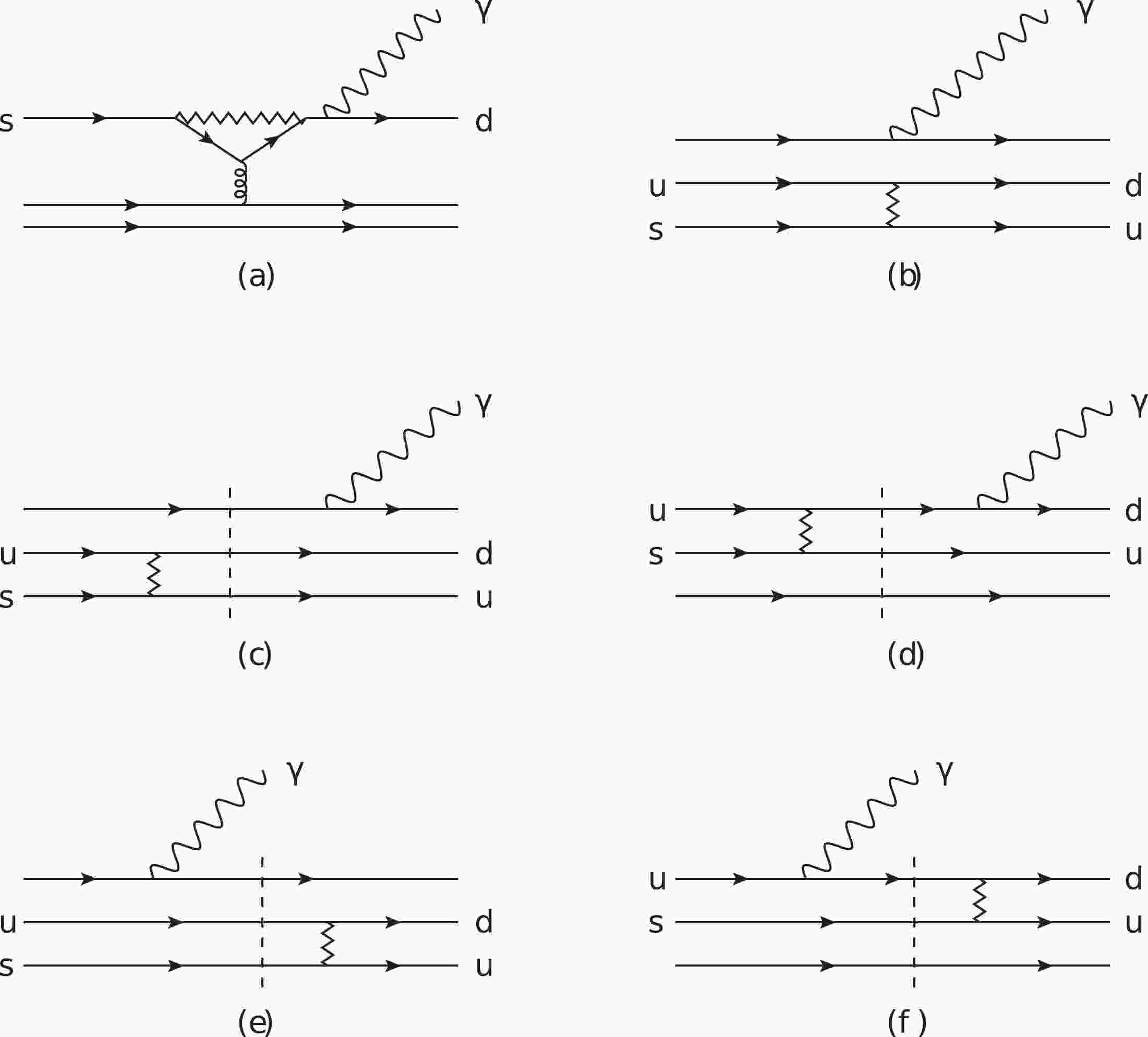
An obvious feature of radiative decays is that the charge is conserved. This suggests that the Cabbibo-allowed weak transition processes occur at leading order, either via a single-quark transition through a penguin diagram, as shown in Fig. 1(a), or via a two-quark transition process through an internal conversion of
$ su\to ud $ , as shown in Figs. 1(b)-(f). The penguin transition is strongly suppressed, primarily because it involves loops; this explains the small partial width of$ \Xi^-\to \Sigma^-\gamma $ . In contrast, the internal conversion processes are tree-level transitions. These are focused in this work.
Figure 1. Typical weak radiative transitions, categorized as follows: (a) is the typical single-quark transition diagram. (b)-(f) are the two-quark transition diagrams, among which (c)-(f) are called pole terms. Note that every diagram actually stands for a group of diagrams, considering that the photon can be emitted by any quark.
The two-quark transition processes can be further categorized into two classes, depending on whether intermediate baryons contribute or not, i.e., the short-distance process and long-distance process. Figure 1(b) illustrates the short-distance process, which stands for a group of diagrams where the photon is radiated from any charged particle. Figures 1(c)-(f) are identified as long-distance processes because intermediate resonances (pole terms) contribute to the transition matrix element. For the hyperon weak decays, the long-distance pole terms become leading contributions because of the closeness of the intermediate baryons to either the initial or final-state baryons. A coarse estimate of the enhancement factor is
$ 2\tilde{M}^2/(M_i^2-M_f^2)\simeq \tilde{M}/(M_i-M_f) $ , which arises from the intermediate propagators with$ \tilde{M}\simeq (M_i+M_f)/2 $ , a mass scale set by the initial and final-state hyperons. We note in advance that, in most cases, there exist cancellations among the pole terms of Figs. 1(c)-(f) [31, 32]. Still, the dominance of the pole terms is evident. We thus only consider the pole contributions in this work. Instead of trying to perfectly describe the available data, we intend to appraise the overall quality of the NRCQM approach. -
Concentrating on the transition amplitudes from the pole terms, the internal conversion via the weak interaction and photon radiation via the EM transition are connected by intermediate baryons. The weak interaction operator can be described by [13, 31, 34]
$ H_W = \frac{G_F}{\sqrt 2}\int {\rm d} {{x}} \frac12 \{ J^{-,\mu}({{x}}),J^{+}_{\mu}({{x}}) \},$

(1) where
$ \begin{aligned} J^{+,\mu}({{x}})& = \left(\begin{array}{cc}\bar u&\bar c \end{array}\right)\cdot\gamma^\mu(1-\gamma_5)\cdot \left(\begin{array}{cc} \cos \theta_C & \sin \theta_C \\ -\sin \theta_C &\cos \theta_C \end{array}\right) \cdot\left( \begin{array}{c} d\\s \end{array}\right), \\ J^{-,\mu}({{x}})& = \left(\begin{array}{cc}\bar d &\bar s \end{array}\right)\cdot \left(\begin{array}{cc} \cos \theta_C & -\sin \theta_C \\ \sin \theta_C &\cos \theta_C \end{array}\right)\cdot \gamma^\mu(1-\gamma_5)\cdot \left( \begin{array}{c} u\\c \end{array}\right). \end{aligned} $

(2) $ H_W $ can be separated into two parts, with either parity-conserving (PC) or parity-violating (PV) behavior, i.e.,$ H_{W}\equiv H_W^{\rm PC}+H_W^{\rm PV} , $

(3) where
$ H_W^{\rm PC}\equiv \frac{G_F}{\sqrt 2} \int \mathrm d {{x}} \left[ j_\mu^{(-)}({{x}})j^{(+)\mu}({{x}}) +j_{5\mu}^{(-)}({{x}})j_5^{(+)\mu}({{x}}) \right], $

(4) $ H_W^{\rm PV}\equiv \frac{G_F}{\sqrt 2} \int \mathrm d {{x}} \left[ j_\mu^{(-)}({{x}})j_5^{(+)\mu}({{x}}) +j_{5\mu}^{(-)}({{x}})j^{(+)\mu}({{x}}) \right]. $

(5) In the non-relativistic limit,
$H_W^{\rm PC,PV}$ , can be reduced to [34]$ \begin{aligned}[b] H_W^{\rm PC} =& \frac{G_F}{\sqrt 2} V_{ud}V_{us} \sum\limits_{i\neq j}\frac{1}{(2\pi)^3} \tau^{(-)}_i \nu^{(+)}_j\\&\times\left( 1- {{{\sigma}}}_i\cdot{{{\sigma}}}_j\right)\delta({{p}}_i^\prime+{{p}}_j^\prime-{{p}}_i-{{p}}_j), \end{aligned} $

(6) and
$ \begin{aligned}[b] H_W^{\rm PV} =& \frac{G_F}{\sqrt 2} V_{ud}V_{us} \sum\limits_{i \neq j }\frac{1}{(2\pi)^3}\delta({{p}}_i^\prime+{{p}}_j^\prime-{{p}}_i-{{p}}_j) \tau^{(-)}_i \nu^{(+)}_j \\ & \times \frac{1}{2m_q} \left\{ -({{\sigma}}_i-{{\sigma}}_j)\cdot[({{p}}_i^\prime-{{p}}_j^\prime)+({{p}}_i-{{p}}_j)]\right.\\&\left. + {\rm i} ({{\sigma}}_i\times{{\sigma}}_j)\cdot[({{p}}_i-{{p}}_j)-({{p}}_i^\prime-{{p}}_j^\prime)] \right\}, \end{aligned} $

(7) where
$ \tau^{(-)} $ and$ \nu^{(+)} $ are flavor changing operators that operate as$ \tau^{(-)}u = d $ and$ \nu^{(+)}s = u $ , respectively. The subscripts$ i, j $ are the quark labels. m is the constituent quark mass. In this work, we take the SU(3) flavor symmetry limit with$ m_q = m_u = m_d = m_s $ .$V_{ud}$ and$V_{us}$ are the Cabbibo-Kobayashi-Maskawa matrix elements.The Hamiltonian for the EM interaction is written as
$ H_{\rm EM} = {\mathsf{e}} \int {\rm d} {{x}} \bar q({{x}})\gamma^\mu q(x)A_\mu({{x}}) \ , $

(8) where
$ {\mathsf{e}} $ is the charge of the quark;$ q({{x}}) $ and$ \bar q({{x}}) $ are the$j^{\rm th}$ quark fields before and after emitting the photon, respectively. In the non-relativistic limit,$H_{\rm EM}$ can be expanded in momentum space as:$ \begin{aligned}[b] H_{\rm EM} = &\sum\limits_j {\mathsf{e}}_j \bar u({{p}}_j^f)\gamma^\mu u({{p}}_j^i)\epsilon_\mu \delta({{p}}^f_j+{{k}} -{{p}}^i_j)\\ = &\frac{1}{(2\pi)^\frac32}\frac{1}{(2k^0)^\frac12}\sum\limits_j {\mathsf{e}}_j \left \{\epsilon_0\!-\!\left[\frac{{{\epsilon}} \cdot {{p}}_j^i}{2m_j}\!+\!\frac{{{\epsilon}} \cdot {{p}}_j^f}{2m_j} \!+\!{\rm i}\frac{{{\sigma}}_j \cdot({{k}}\times {{\epsilon}}) }{2m_j}\right ] \right\}\\&\times \delta({{p}}_j^f+{{k}} -{{p}}_j^i), \\[-16pt]\end{aligned} $

(9) where
$ m_j $ and$ {\mathsf{e}}_j $ are the mass and charge of the$j^{\rm th}$ quark, respectively;$ {{p}}^i_j $ and$ {{p}}^f_j $ denote the three-vector momentum carried by the$j^{\rm th}$ quark before and after emitting the photon, respectively;$ {{k}} $ is the photon momentum, and$ (\epsilon_0,{{\epsilon}}) $ is its polarization. For a real emitted photon, only the transverse polarizations can contribute.$H_{\rm EM}$ can thus be reduced to$ \begin{aligned}[b] H_{\rm EM} =& -\frac{1}{(2\pi)^\frac32}\frac{1}{(2k^0)^\frac12}\sum\limits_j {\mathsf{e}}_j \left[\frac{{{\epsilon}} \cdot {{p}}^i_j}{m_j}+{\rm i}\frac{{{\sigma}}_j \cdot({{k}}\times {{\epsilon}}) }{2m_j}\right] \\&\times \delta^3({{p}}_j^f+{{k}} -{{p}}_j^i). \end{aligned}$

(10) The first term contributes to the electric-dipole transition, which could raise or decrease the orbital angular momentum by one unit, and the second term contributes to the magnetic-dipole transition, which could raise or decrease the spin of the
$j^{\rm th}$ quark by one unit [13, 31, 34]. -
With the operators defined in the previous subsection, we can calculate the pole terms in the NRCQM framework. We take the direction of the photon momentum as the z-axis, i.e.,
$ k^0 = k $ and$ {{k}} = (0, \ 0, \ k) $ are the energy and three momentum of the photon, respectively. The energy and momentum of the initial and final baryon are noted as$ (E_i, \ {{P}}_i) $ and$ (E_f, \ {{P}}_f) $ , respectively. In the rest frame of the initial baryon, we have$ {{P}}_i = 0 $ and$ {{k}} = -{{P}}_f $ .The nonlocal operators for the weak and EM transitions will distinguish processes between Figs. 1(c) and (e) (or between Figs. 1(d) and (f)). With the baryon wavefunctions constructed on the basis of SU(6)
$ \otimes $ O(3) symmetry and by separately calculating the weak internal conversion and EM transition couplings, Figs. 1(c) and (e) together will be evaluated explicitly with the quark labels tagged to the interacting quarks, and similarly, Figs. 1(d) and (f) will be evaluated. Note that in the literature, e.g., [18], Figs. 1(c) and (d) (or Figs. 1(e) and (f)) are sometimes treated as two different transition processes according to whether or not the EM transition operator is involved in the weak internal conversion process. If the symmetry is properly accounted for regarding both wavefunctions and operators, in principle, there is no need to distinguish between Figs. 1(c) and (d), or between (e) and (f). For convenience, we label the amplitudes of Figs. 1(c)-(d) and Figs. 1(e)-(f) by the subscripts A and B, respectively.Proceeding to the calculation of the full transition amplitudes, we separate the parity-conserving and parity-violating parts as follows:
$ {\cal M} = {\cal M}({{\epsilon}},S_f^z,S_i^z) = {\cal M}_{\rm PC}+ {\cal M}_{\rm PV}, $

(11) where
$ S_f^z $ and$ S_i^z $ are the third component of the spin of the final baryon and initial baryon, respectively, and are omitted to simplify the representation. Also omitted is the photon polarization$ {{\epsilon}} = \mp (1,\pm i,0)/\sqrt2 $ . Owing to the symmetries and hermiticity of the Hamiltonian, the amplitudes corresponding to the two possible polarizations are related, and it is sufficient to perform the calculation with the polarization$ {{\epsilon}} = -(1,i,0)/\sqrt2 $ , abbreviated as "+". The parity-conserving amplitude${\cal M}_{\rm PC}$ and parity-violating amplitude${\cal M}_{\rm PV}$ are then given by the pole terms via the process A or B, i.e.,$ {\cal M}_{\rm PC} = {\cal M}_{{\rm PC},A}+ {\cal M}_{{\rm PC},B}, $

(12) $ {\cal M}_{\rm PV} = {\cal M}_{{\rm PV},A}+ {\cal M}_{{\rm PV},B}, $

(13) where
$\begin{aligned}[b] {\cal M}_{{\rm PC},A}\equiv& \sum\limits_{B_m} \left\langle B_f({{P}}_f,S_f^z) \middle| H_{\rm EM} \middle| B_m({{P}}_i,S_i^z) \right\rangle \\&\times\frac{{\rm i}}{\not\!\! p_{B_m} -M_{B_m}+\frac{\rm i}{2}\Gamma_{B_m}} \left\langle B_m({{P}}_i,S_i^z) \middle| H_W^{\rm PC} \middle| B_i({{P}}_i,S_i^z) \right\rangle,\end{aligned} $

(14) $\begin{aligned}[b] {\cal M}_{{\rm PV},A}\equiv& \sum\limits_{B'_m} \left\langle B_f({{P}}_f,S_f^z) \middle| H_{\rm EM} \middle| B'_m({{P}}_i,S_i^z) \right\rangle \\&\times\frac{{\rm i}}{\not\!\! p_{B'_m} -M_{B'_m}+\frac{{\rm i}}{2}\Gamma_{B'_m}} \left\langle B'_m({{P}}_i,S_i^z) \middle| H_W^{\rm PV} \middle| B_i({{P}}_i,S_i^z) \right\rangle, \end{aligned}$

(15) $\begin{aligned}[b] {\cal M}_{{\rm PC},B}\equiv& \sum\limits_{B_m} \left\langle B_f({{P}}_f,S_f^z) \middle| H_{W}^{\rm PC} \middle| B_m({{P}}_f,S_f^z) \right\rangle \\&\times\frac{{\rm i}}{\not\!\! p_{B_m} -M_{B_m}+\frac{{\rm i}}{2}\Gamma_{B_m}} \left\langle B_m({{P}}_f,S_f^z) \middle| H_{\rm EM} \middle| B_i({{P}}_i,S_i^z) \right\rangle,\end{aligned} $

(16) $\begin{aligned}[b]{\cal M}_{{\rm PV},B}\equiv& \sum\limits_{B'_m} \left\langle B_f({{P}}_f,S_f^z) \middle| H_{W}^{\rm PV} \middle| B'_m({{P}}_f,S_f^z) \right\rangle\\&\times \frac{{\rm i}}{\not\!\! p_{B'_m} -M_{B'_m}+\frac{{\rm i}}{2}\Gamma_{B'_m}} \left\langle B'_m({{P}}_f,S_f^z) \middle| H_{\rm EM} \middle| B_i({{P}}_i,S_i^z) \right\rangle, \end{aligned}$

(17) where a complete set of intermediate baryon states
$ B_m $ ($ B_m' $ ) with quantum numbers$ 1/2^+ $ ($ 1/2^- $ ) has been included in processes A and B, respectively.$\langle B | H_{W}^{\rm PC/PV} | B'\rangle$ and$\langle B| H_{\rm EM} | B' \rangle$ are the weak and EM transition matrix elements, respectively. The weak matrix elements are calculated in a manner similar to that reported in Refs. [32, 33]. In the following, we provide some details about the calculations of the EM transition matrix elements.Taking advantage of the fact that we use baryon wave functions that are fully symmetric with respect to the space, spin, and flavor degrees of freedom (see Appendix),
$H_{\rm EM}$ can be replaced by$\begin{aligned}[b] H^{+}_{\rm EM} =& \sum\limits_j (H_{\rm EM}^+)_j \to 3(H_{\rm EM}^+)_1\\ =& -\frac{1}{(2\pi)^\frac32}\frac{1}{(2k^0)^\frac12}\frac{3 {\mathsf{e}}_1}{\sqrt2 m_1} \\&\times\left[p_1^+ +\sigma_1^+ k \right] \delta^3({{p}}_1^f+{{k}} -{{p}}_1^i),\end{aligned} $

(18) where
$ p^+\equiv p_x+{\rm i}p_y, \quad \sigma^+\equiv \frac{\sigma_x+{\rm i}\sigma_y}{2}. $

(19) Taking the decay of
$ \Lambda\to \gamma n $ of the A-type as an example, the EM transition amplitude can be obtained as$ \begin{aligned}[b] & \left\langle B_f({{P}}_f,S_f^z)\middle | H_{\rm EM}^+ \middle | B_i({{P}}_i,S_i^z) \right\rangle \\ =& \left\langle \frac{1}{\sqrt2}(\phi_n^\rho\chi_{1/2,S_f^z}^\rho+\phi_n^\lambda\chi_{1/2,S_f^z}^\lambda)\Phi^{00;00}_{00}({{p}}_1^f,{{p}}_2^f,{{p}}_3^f) \Biggr| H_{\rm EM}^+ \right.\\&\times\Biggr |\left. \frac{1}{\sqrt2}(\phi_n^\rho\chi_{1/2,S_i^z}^\rho+\phi_n^\lambda\chi_{1/2,S_i^z}^\lambda)\Phi^{00;00}_{00}({{p}}_1^i,{{p}}_2^i,{{p}}_3^i) \right\rangle \\ = &C \langle\Phi^{00;00}_{00}(\{{{p}}_j^f\})|p^+_1|\Phi^{00;00}_{00}(\{{{p}}_j^i\})\rangle\\&+ D \langle\Phi^{00;00}_{00}(\{{{p}}_j^f\})|k|\Phi^{00;00}_{00}(\{{{p}}_j^i\})\rangle. \end{aligned} $

(20) Here
$ \Phi({{p}}_1,{{p}}_2,{{p}}_3) = \Psi({{P}},{{p}}_\rho,{{p}}_\lambda) $ is the wavefunction written in terms of individual momenta and spelled out in the Appendix as a function of the Jacobi coordinates, and its indices denote both the internal and global radial and orbital excitations. Accordingly, the two last brackets are the matrix elements of these spatial wave functions in momentum space, and the coefficients C and D are the factors extracted in the spin-isospin space. The first term will raise the orbital angular momentum projection of the interacting quark by one unit, and the second one will raise its spin projection by one unit. A general definition of the convolution integral is as follows:$ \begin{split} \langle \cdots O(p) \cdots \rangle&{} = I_{n_\rho^f \ell_\rho^f;n_\lambda^f\ell_\lambda^f;L^f M^f;n_\rho^i \ell_\rho^i;n_\lambda^i \ell_\lambda^i;L^i M^i}(O(p))\\ &{} = \int {\rm d}^{(3)}{{p}}^f d^{(3)}{{p}}^i \delta^3({{p}}_1^f+{{k}} -{{p}}^i_1)\delta^3({{p}}_2^f-{{p}}_2^i)\\ &{} \quad\times \delta^3({{p}}_3^f-{{p}}_3^i)\Phi^*{\,}_{L^f M^f}^{n_\rho^f\ell_\rho^f;n_\lambda^f{}\ell_\lambda^f}({{p}}_1^f,{{p}}_2^f,{{p}}_3^f) O(p)\\ &{} \quad\times \Phi_{L^i M^i}^{n_\rho^i\ell_\rho^i;n_\lambda^i{}\ell_\lambda^i}({{p}}_1^i,{{p}}_2^i,{{p}}_3^i), \\[-15pt]\end{split} $

(21) where
$ O(p) $ is a function of quark momenta, such as$ p_1^+ $ and k. For the transitions between two ground states, it is easy to verify that$ I(p^+_1) = 0,\qquad I(k) = k {\rm e}^{-\genfrac{}{}{}{1}{k^2}{6 \alpha ^2}}.$

(22) This indicates that only the term proportional to D, namely the magnetic-dipole part of
$H^+_{\rm EM}$ in Eq. (20), can contribute to the transitions between the two ground states. With fixed spin projections in the initial and final states, i.e.,$ S_i^z = -1/2 $ and$ S_f^z = 1/2 $ , coefficient D can be calculated in the spin-flavor space:$ \begin{split}D=& -\frac{3}{(2\pi)^\frac32}\frac{1}{(2k^0)^\frac12} \left\langle \frac{1}{\sqrt2}\left(\phi_n^\rho\chi_{1/2,1/2}^\rho+\phi_n^\lambda\chi_{1/2,1/2}^\lambda \right) \Biggr|\frac{ {\mathsf{e}}_1 \sigma^+_1}{\sqrt2 m_1} \right.\\ &\times \Biggr|\left.\frac{1}{\sqrt2}\left(\phi_n^\rho\chi_{1/2,-1/2}^\rho+\phi_n^\lambda\chi_{1/2,-1/2}^\lambda \right) \right\rangle \\ =& \frac{ {\mathsf{e}}}{6 \sqrt{2} \pi ^{3/2} \sqrt{k^0} m_q}. \\[-13pt]\end{split} $

(23) Finally, we have
$ \left\langle n \left({{P}}_f,\frac12 \right) \middle | H_{\rm EM}^+ \middle | n\left({{P}}_i,-\frac12\right) \right\rangle = \frac{ {\mathsf{e}} k}{6 \sqrt{2} \pi^{3/2} \sqrt{k^0} m_q} {\rm e}^{-\genfrac{}{}{}{1}{k^2}{6 \alpha ^2}}. $

(24) Analogously, the radiative transitions between the intermediate
$ 1/2^- $ baryon and final$ 1/2^+ $ baryon can be calculated. In such processes, the contributions will come from the term proportional to C in Eq. (20). The wavefunctions and detailed expressions of the transition amplitudes are provided in the Appendix.With the explicit amplitudes for the PC and PV transitions, the partial decay width for the hyperon weak radiative decays can be obtained as follows:
$ \Gamma = 8\pi^2 \frac{|{\bf{k}}| k^0 E_f}{M_i}\frac{1}{2S_i+1}\sum\limits_{S_f^z,S_i^z} 2\left(| {\cal M}^{+,S_f^z,S_i^z}_{\rm PC}|^2 + | {\cal M}^{+,S_f^z,S_i^z}_{\rm PV}|^2\right), $

(25) where
$ {\cal M}^{+,S_f^z,S_i^z}_{\rm PC} $ and$ {\cal M}^{+,S_f^z,S_i^z}_{\rm PV} $ are the PC and PV amplitudes, respectively, with the photon polarization$ {{\epsilon}} ^+ $ , and$ S_i $ and$ M_i $ are the spin and mass of the initial baryon, respectively.The parity asymmetry parameter can be extracted in the quark model. Generally, the amplitude of the hyperon weak radiative decay at the hadron level has the following form:
$ {\cal M} = G_F \frac{ {\mathsf{e}}}{\sqrt{4\pi}}\epsilon_\mu \bar u(p')(A+B\gamma_5)\sigma^{\mu\nu}q_\nu u(p), $

(26) where
$ \epsilon_\mu $ is the polarization vector of the photon;$ u(p) $ and$ \bar u(p') $ are the spinors of the initial-state hyperon and final-state nonstrange baryon, respectively. A and B represent the PC (P-wave) and PV (S-wave) amplitudes, respectively. The asymmetry parameter is defined as follows:$ \alpha_\gamma\equiv \frac{2 {\rm{Re}}(A^*B)}{|A|^2+|B|^2}. $

(27) By matching A and B to the quark model amplitudes, the asymmetry parameter
$ \alpha_\gamma $ can be expressed in terms of the quark model amplitudes for the PC and PV transitions, i.e.,$ \alpha_\gamma = \frac{2 {\rm{Re}}( {\cal M}_{\rm PC}^* {\cal M}_{\rm PV})}{| {\cal M}_{\rm PC}|^2+| {\cal M}_{\rm PV}|^2}. $

(28) With this asymmetry parameter, the angular distribution of the final-state baryon in the rest frame of the initial hyperon can be written as follows:
$\frac{{\rm d} N}{{\rm d} \Omega} = \frac{N}{4\pi}\left (1+\alpha_\gamma {{P}}_h \cdot \hat{{{p}}} \right ), $

(29) where
$ {{P}}_h $ is the polarization vector of the decaying hyperon, and$ \hat{{{p}}} $ is the direction of the three-vector momentum of the final-state baryon.The following processes are included in this work:
$ \Lambda \to n \gamma $ ,$ \Sigma^+\to p\gamma $ ,$ \Sigma^0\to n\gamma $ ,$ \Xi^0 \to \Lambda\gamma $ , and$ \Xi^0 \to \Sigma^0 \gamma $ . Although the partial width of$ \Sigma^0\to \Lambda \gamma $ is saturated by the EM interaction, we still evaluate the weak radiative decay contribution here as a comparison with the EM process. -
These weak radiative decay processes, i.e.,
$ \Lambda \to n \gamma $ ,$ \Sigma^+ \to p \gamma $ ,$ \Sigma^0 \to n \gamma $ ,$ \Xi^0 \to \Lambda\gamma $ , and$ \Xi^0 \to \Sigma^0\gamma $ , are all Cabbibo-favored with$ |\Delta I| = 1/2 $ and$ |\Delta s| = 1 $ transitions. The dominance of the pole terms in the transition amplitudes suggests that all the intermediate states of$ J^P = 1/2^+ $ with the proper flavor should be included for the PC amplitude, while all the states of$ 1/2^- $ should be included for the PV one. However, taking into account the propagator suppression effects when the intermediate states become highly off-shell, we only consider the first orbital excitation states for the PV amplitude. This approximation will introduce some uncertainties to the final results. Taking the$ \Lambda $ decays as an example, the upper limit of the uncertainties can be estimated by the ratios$R_{\rm PC} = |(M_\Lambda^2-M_p^2)/(M_\Lambda^2-M_{N^*(1440)}^2)|^2\simeq 0.20$ for the PC part in the branching ratio, and$R_{\rm PV} = |(M_\Lambda(1405)^2-M_p^2)/ (M_{\Lambda(L = 3)}^2-M_p^2)|^2\simeq 0.12$ for the PV part in the branching ratio. Here,$ N^*(1440) $ is the first radial excitation state of the nucleon, and$ \Lambda(L = 3) $ denotes the second negative parity orbital excitation state of$ \Lambda $ . The multiplets with$ L = 3 $ have not yet been established experimentally, so we adopt$ M_{\Lambda(L = 3)} = 2 $ GeV for its mass as a conservative estimate. Theoretical calculations in the literature suggest that their masses are well above 2 GeV [35] (see also Ref. [36] for a review of baryon spectroscopy in the quark model and references therein).The intermediate states considered in this work are listed in Table 1. These states are either ground states with
$ J^P = 1/2^+ $ or first orbital excitations with$ J^P = 1/2^- $ . For the$ 1/2^- $ intermediate hyperons,$ \Lambda(1405) $ is assigned as the flavor singlet in the representation$ [70,^21] $ . For multiplets of representations$ [70,^28] $ and$ [70,^48] $ , the corresponding states have not yet been determined experimentally. Although the quantum numbers of$ \Xi(1620) $ and$ \Xi(1690) $ have not been measured in experiments, they are considered to belong to representations$ [70,^28] $ and$ [70,^48] $ , respectively.PC $ [56,^28] $ 

p n $ \Lambda $ 

$ \Xi^0 $ 

$ 0.94 $ 

$ 0.94 $ 

$ 1.12 $ 

$ 1.31 $ 

$ \Sigma^+ $ 

$ \Sigma^0 $ 

$ 1.20 $ 

$ 1.20 $ 

PV $ [70,^28] $ 

$ N(1535) $ 

$ \Lambda(1670) $ 

$ \Sigma(1620) $ 

$ \Xi(1620) $ 

$ 1.53(0.15) $ 

$ 1.67(0.035) $ 

$ 1.62(0.05) $ 

$ 1.62(0.03) $ 

$ [70,^48] $ 

$ N(1650) $ 

$ \Lambda(1800) $ 

$ \Sigma(1750) $ 

$ \Xi(1690) $ 

$ 1.655(0.135) $ 

$ 1.8(0.3) $ 

$ 1.75(0.15) $ 

$ 1.62(0.03) $ 

$ [70,^{{2}}{}{{10}}] $ 

$ \Delta(1620) $ 

1.61(0.13) Table 1. Intermediate states considered in our calculation. The baryon masses and decay widths (given in the brackets) are taken from PDG [37] (in units of GeV). Only the central values of the masses and widths are listed.
With the EM and weak coupling matrix elements for the
$ 1/2^+ $ and$ 1/2^- $ states calculated in the NRCQM, we can obtain the analytical amplitudes for each pole term; they are provided in Appendix C. One can see that the PC amplitudes are given by the intermediate$ 1/2^+ $ octet baryons, and the decays are given through a P wave, while the parity-violating ones are given through an S wave.In our framework, the input parameters include the constituent quark masses and harmonic oscillator strengths. In the present calculations, we take the SU(3) flavor symmetry for the constituent quark masses, i.e.,
$ m_q = m_u = m_d = m_s = 0.35 $ GeV, as the leading order approximation. This simplifies the baryon wavefunctions at this moment. Because the three-vector momentum carried by the photon is rather small, this approximation does not cause significant uncertainty in the numerical results. In contrast, the numerical results are more sensitive to the harmonic oscillator strengths, i.e.,$ \alpha_\rho $ and$ \alpha_\lambda $ for the$ \rho $ and$ \lambda $ degrees of freedom in the Jacobi coordinate, respectively. In the equal mass limit of$ m_u = m_d = m_s $ , these two parameters satisfy$ \alpha_\rho = \alpha_\lambda\equiv \alpha $ . One can see later that the analytical amplitudes will be proportional to$ \alpha^3 $ . Thus, more uncertainties can arise from the harmonic oscillator strength$ \alpha $ . Considering that$ \Xi $ contains two s quarks, the SU(3) flavor symmetry breaking effect should not be ignored, so we adopt a different value for the oscillator strength of the$ \Xi $ decays. Thus, in the numerical studies, we adopt$ \alpha = 0.45 $ GeV for the$ \Lambda $ and$ \Sigma $ decays and$ \beta = 0.38 $ GeV for the$ \Xi $ decays.The numerical results of amplitudes are given in Table 2. Some general features can be understood as follows.
Process PCA PVA PCB PVB Total (PC) Total (PV) $ \Lambda \to n\gamma $ 

n $ -6.68 $ 

$ N(1535) $ 

$-4.72-0.99{\rm i}$ 

$ \Lambda $ 

$ 3.97 $ 

$ \Lambda(1670) $ 

$-1.54-0.047{\rm i}$ 

$ 5.82 $ 

$-14.91-1.48{\rm i}$ 

$ N(1650) $ 

$0.22+0.032{\rm i}$ 

$ \Sigma^0 $ 

$ 8.53 $ 

$ \Lambda(1800) $ 

$0.072-0.017{\rm i}$ 

$ \Delta(1620) $ 

$ 0 $ 

$ \Lambda(1405) $ 

$-4.27-0.28{\rm i}$ 

$ \Sigma(1620) $ 

$-4.91-0.23{\rm i}$ 

$ \Sigma(1750) $ 

$ 0.24 $ 

$ \Sigma^+\to p\gamma $ 

p $ -19.06 $ 

$ N(1535) $ 

$-9.65-2.39{\rm i}$ 

$ \Sigma^+ $ 

$ 24.16 $ 

$ \Sigma(1620) $ 

$-5.75-0.27{\rm i}$ 

$ 5.10 $ 

$-15.40-2.66{\rm i}$ 

$ N(1650) $ 

$ 0 $ 

$ \Sigma(1750) $ 

$ 0 $ 

$ \Delta(1620) $ 

$ 0 $ 

$ \Sigma^0\to n\gamma $ 

n $ 8.93 $ 

$ N(1535) $ 

$7.69+1.92{\rm i}$ 

$ \Lambda $ 

$ -7.91 $ 

$ \Lambda(1670) $ 

$2.15+0.066{\rm i}$ 

$ 6.69 $ 

$1.33+1.37{\rm i}$ 

$ N(1650) $ 

$-0.68-0.15{\rm i}$ 

$ \Sigma^0 $ 

$ 5.67 $ 

$ \Lambda(1800) $ 

$-0.20-0.046{\rm i}$ 

$ \Delta(1620) $ 

$ 0 $ 

$ \Lambda(1405) $ 

$-5.58-0.36{\rm i}$ 

$ \Sigma(1620) $ 

$-2.28-0.11{\rm i}$ 

$ \Sigma(1750) $ 

$ 0.22 $ 

$ \Xi^0\to \Lambda\gamma $ 

$ \Lambda $ 

$ 5.79 $ 

$ \Lambda(1670) $ 

$4.73+0.26{\rm i}$ 

$ \Xi^0 $ 

$ -13.60 $ 

$ \Xi(1620) $ 

$6.33+0.22{\rm i}$ 

$ -7.81 $ 

$-4.38-3.88{\rm i}$ 

$ \Sigma^0 $ 

$ 0 $ 

$ \Lambda(1800) $ 

$-0.23-0.083{\rm i}$ 

$ \Xi(1690) $ 

$-0.46-0.014{\rm i}$ 

$ \Lambda(1405) $ 

$-14.7-4.26{\rm i}$ 

$ \Sigma(1620) $ 

$ 0 $ 

$ \Sigma(1750) $ 

$ 0 $ 

$ \Xi^0\to \Sigma^0\gamma $ 

$ \Lambda $ 

$ -8.15 $ 

$ \Lambda(1670) $ 

$-10.75-0.59{\rm i}$ 

$ \Xi^0 $ 

$ 0 $ 

$ \Xi(1620) $ 

$ 0 $ 

$ -8.15 $ 

$-45.65-10.67{\rm i}$ 

$ \Sigma^0 $ 

$ 0 $ 

$ \Lambda(1800) $ 

$0.21+0.074{\rm i}$ 

$ \Xi(1690) $ 

$ 0 $ 

$ \Lambda(1405) $ 

$-35.11-10.15{\rm i}$ 

$ \Sigma(1620) $ 

$ 0 $ 

$ \Sigma(1750) $ 

$ 0 $ 

Table 2. Numerical results of amplitudes for every channel, in units of
$ (10^{-10}\; {\rm{GeV}}^{-1/2}) $ . -
For the processes
$ \Sigma^+\to p\gamma $ and$ \Lambda \to n \gamma $ , it appears that the A- and B-type processes have a destructive interference in the the PC channels, but become constructive in the PV channels. This results in the value of the PC amplitudes becoming smaller than the value of the PV ones for these two decays. Furthermore, this leads to a large value for the asymmetry parameter.It is interesting to note that the PV amplitude of the
$ N(1650) $ , which is assigned as the SU(6) representation$ [70,^48] $ with$ J^P = 1/2^- $ , vanishes in$ \Sigma^+\to p\gamma $ but contributes to the neutral channels of$ \Lambda \to n \gamma $ and$ \Sigma^0\to n\gamma $ . This is understandable via the EM coupling between the$ N^* $ of$ [70,^48] $ and proton$ [56,^28] $ . In such an EM transition process, the so-called “Moorhouse selection rule” [38] should play a role, preventing the intermediate$ N(1650) $ from decaying into$ p\gamma $ .To be more specific, one can prove that the
$ \rho $ mode decays or excitations between states of$ [70,^48] $ and$ [56,^28] $ via the EM transition operator vanish. Because the spin and orbital angular momentum operators are symmetric with respect to the quark indices of the first two quarks, the$ \rho $ mode spatial wavefunction of$ [70,^48] $ cannot orbitally decay into a symmetric spatial wavefunction of$ [56,^28] $ . The$ \lambda $ mode decays or excitations between states of$ [70,^48] $ and$ [56,^28] $ are, in principle, allowed. However, for the charged channel of$ N^*([70,^48])\to p\gamma $ , one has$ \langle \phi^\lambda_{N^{*+}}|\Sigma_{i = 1}^3 {\mathsf{e}}_i|\phi^\lambda_p\rangle = 3\langle \phi^\lambda_{N^{*+}} | {\mathsf{e}}_3|\phi^\lambda_p\rangle = 0 $ . Thus, the$ \lambda $ mode is also forbidden.It should be noted that representations of
$ [70,^48] $ and$ [70,^28] $ in the first orbital excitations can mix, and the physical states$ N(1535) $ and$ N(1650) $ are actually mixing states of these two configurations. As a consequence, both states can actually contribute to$ \Sigma^+\to p\gamma $ . This is an interesting phenomenon that may provide an alternative way to study the structure of these two resonances.A similar relation also appears in the EM transitions of the PV B-type process, i.e., the EM transitions between
$ \Sigma^+ $ of$ [56,^28] $ and$ \Sigma^{*+} $ of$ [70,^48] $ . Again, one can prove that only the$ \lambda $ mode of transitions is allowed. However, with$ \langle \phi^\lambda_{\Sigma^{*+}}|\Sigma_{i = 1}^3 {\mathsf{e}}_i|\phi^\lambda_{\Sigma^+}\rangle = 3\langle \phi^\lambda_{\Sigma^{*+}}| {\mathsf{e}}_3|\phi^\lambda_{\Sigma^+}\rangle = 0 $ , the$ \lambda $ mode of transitions will also be forbidden. Thus, states of$ [70,^48] $ do not contribute to the PV amplitude in$ \Sigma^+\to p\gamma $ .It is also clear that the states of
$ [70,^{{2}}{}{{10}}] $ do not contribute to the octet radiative weak decays. This is due to the requirement of the$ \rho $ mode orbital excitations between the spatial wavefunctions of$ [70,^{{2}}{}{{10}}] $ and$ [56,^28] $ in association with the spin-flavor operators in Eq. (7), which are nonvanishing between$ \lambda $ and$ \rho $ modes. As a consequence, the two terms in Eq. (7) exactly cancel out. This vanishing transition was listed in Ref. [15] but was not discussed much there. Note that the transition$ \Sigma^+\to p\gamma $ does not violate the$ |\Delta I| = 1/2 $ rule. The vanishing contribution of the$ \Delta(1620) $ of representation$ [70,^{{2}}{}{{10}}] $ can be regarded as a kind of dynamic selection rule in the quark model. In fact, this selection rule also plays a role in the hadronic weak decays of$ \Sigma\to N\pi $ and$ \Lambda\to N\pi $ . A recent study can be found in Ref. [33]. -
The situation in
$ \Xi^0\to \Sigma^0 \gamma $ and$ \Lambda \gamma $ is different from that in$ \Lambda $ and$ \Sigma $ decays. Here, the contributions from the PC processes are larger than those from the destructive PV ones.It is noticeable that the B-type amplitudes in
$ \Xi^0 \to \Sigma^0 \gamma $ vanish for both PC and PV transitions. Meanwhile, the intermediate$ \Sigma^{(*)} $ states do not contribute to the A-type transitions. These are due to the weak interaction operators. Note that the flavor transition element vanishes:$ \langle \phi_{\Sigma^0}^\rho|\tau_1^{(-)}\nu_2^{(+)}|\phi_{\Xi^0}^\rho\rangle = 0 $ . In the PC B-type transition, this leaves the$ \lambda $ mode to contribute. However, one finds that the spin transition element$ \langle\chi_{\frac 12 S_z}^\lambda|(1-{{{\sigma}}}_1\cdot{{{\sigma}}}_2) |\chi_{\frac 12 S_z}^\lambda\rangle = 0 $ , with the spins of the first two quarks in parallel. Therefore, the intermediate$ \Sigma^0 $ does not contribute to the PC amplitude.For the PV A-type transitions, the intermediate
$ \Sigma^{*0} $ belongs to either representation$ [70,^28] $ or$ [70,^48] $ . Again, with$ \langle \phi_{\Sigma^0}^\rho|\tau_1^{(-)}\nu_2^{(+)}|\phi_{\Xi^0}^\rho\rangle = 0 $ , it leaves the wavefunction component$ \phi_{\Sigma^0}^\lambda(\chi_{\frac 12 S_z}^\rho\psi_{11L_z}^\rho({{{\rho}}}, {{{\lambda}}})-\chi_{\frac 12 S_z}^\lambda\psi_{11L_z}^\lambda({{{\rho}}}, {{{\lambda}}})) $ of$ [70,^28] $ to be considered. From the PV operators in Eq. (7), one can easily prove that only the transitions between$ \rho $ and$ \lambda $ modes in the spin and spatial spaces can survive. However, the two terms in Eq. (7) have the same average values but opposite signs. They will thus cancel and lead to vanishing contributions from the intermediate$ \Sigma^{*0} $ of$ [70,^28] $ . For the intermediate$ \Sigma^{*0} $ of$ [70,^48] $ , one finds that the corresponding spatial transitions between the$ \rho $ mode will vanish.For the B-type transitions, the intermediate
$ \Xi^{(*)0} $ can be in either$ [56,^28] $ (PC) or$ [70,^28] $ (PV). Their transitions into the final$ \Sigma^0 $ vanish for the same reason, arising from the weak transition operators. Thus, we have the interesting result that all the$ \Xi^{(*)0} $ pole terms in the B-type processes and all the$ \Sigma^0 $ pole terms in the A-type ones vanish in$ \Xi^0 \to \Sigma^0 \gamma $ . -
Proceeding to the calculation of experimental observables, the calculated branching ratios and parity asymmetry parameters are listed in the last columns of Tables 3 and 4, respectively, in comparison with other models. As shown in Table 3, the central values of the branching ratios are similar to the experimental results, except for
$ \Xi^0\to \Sigma^0 \gamma $ . By introducing 0.5% errors to the quark model parameters, i.e.,$ \alpha,\; \beta $ and$ m_q $ , we can estimate the uncertainties of our model calculations. The results show that the uncertainties with the branching ratios are approximately 40%$ \sim $ 50% for each channel, which means that the amplitudes are sensitive to the quark model parameters. This is understandable because the amplitudes are proportional to$ \alpha^3/m_q $ ($ \beta^3/m_q $ ). In contrast, the uncertainties with the asymmetry parameter are relatively smaller. As seen from the expression of Eq. (28) for$ \alpha_\gamma $ , the uncertainties arising from the dependence of$ \alpha^3/m_q $ or$ \beta^3/m_q $ are largely cancelled out.$ B_i\to B_f \gamma $ 

PDG data [37] Broken SU(3) [11] ChPT [25] Pole model [17] Pole model [15] Our result $ \Sigma^+\to p\gamma $ 

$ (1.23\pm0.05) $ 

$ 0.72 $ 

$ \approx 16 $ 

$ 0.75\pm0.30 $ 

$ 1.15 $ 

$ 1.06\pm0.59 $ 

$ \Lambda\to n\gamma $ 

$ (1.75\pm0.15) $ 

$ 0.77 $ 

$ \approx 1.45 $ 

$ 0.16\pm0.06 $ 

$ 0.62 $ 

$ 1.83\pm0.96 $ 

$ \Xi^0\to\Lambda\gamma $ 

$ (1.17\pm0.07) $ 

$ 1.02 $ 

$ \approx 1.17 $ 

$ 0.72\pm0.42 $ 

$ 3.0 $ 

$ 0.96\pm0.32 $ 

$ \Xi^0\to\Sigma^0\gamma $ 

$ 3.33\pm0.1 $ 

$ 4.42 $ 

$ \approx 1.14 $ 

$ 2.6\pm1.2 $ 

$ 7.2 $ 

$ 9.75\pm4.18 $ 

$ \Sigma^0\to n\gamma $ 

− − $ \approx 10^{-9} $ 

$ 1.8\times10^{-9} $ 

$ 10^{-10} $ 

$ \approx 10^{-10} $ 

Table 3. Calculated branching ratios (in units of
$ 10^{-3} $ ) compared with experimental data and other theoretical predictions. In Ref. [25], the results are given by decay width.Note that there are only a limited number of parameters under the NRCQM framework. The overall quality of our model calculations turns out to be reasonable. Our results indicate that the lowest lying states play an essential role through the intermediate pole terms, which is consistent with the results of ChPT [25] and previous quark model calculations [15].
In Table 4, one can see that the signs of the asymmetry parameters are quite different. Our model gives the correct signs for the
$ \Sigma^+ $ and$ \Lambda $ channel and prefers a large value. However, for the$ \Xi^0 $ channels, the sign of the asymmetry parameter is opposite to that of the experimental data. The sign of the asymmetry parameter of$ \Sigma^0\to n \gamma $ is positive, which is opposite to that of the other model calculations [15, 17].$ B_i\to B_f \gamma $ 

PDG [37] Broken SU(3) [11] ChPT [25] Pole model (I) [17] Pole model (II) [15] Our result $ \Sigma^+\to p\gamma $ 

$ -0.76\pm0.08 $ 

$ -0.67 $ 

$ -0.49 $ 

$ -0.92 $ 

$ -0.80 $ 

$ -0.58\pm0.060 $ 

$ \Lambda\to n\gamma $ 

− $ -0.93 $ 

$ -0.19 $ 

$ 0.91 $ 

$ -0.49 $ 

$ -0.67\pm0.060 $ 

$ \Xi^0\to\Lambda\gamma $ 

$ (-0.70\pm0.07) $ 

$ -0.97 $ 

$ 0.46 $ 

$ 0.07 $ 

$ -0.78 $ 

$ 0.72\pm0.11 $ 

$ \Xi^0\to\Sigma^0\gamma $ 

$ (-0.69\pm0.06) $ 

$ -0.92 $ 

$ 0.15 $ 

$ -0.75 $ 

$ -0.96 $ 

$ 0.33\pm0.036 $ 

$ \Sigma^0\to n\gamma $ 

− − − $ -0.65 $ 

$ -0.98 $ 

$ 0.37\pm0.035 $ 

Table 4. Numerical results of the asymmetry parameter compared with experimental data and other theoretical predictions.
In Table 5, we also list the partial decay widths in comparison with the PDG values [37]. Note that the calculated partial decay width of
$ \Sigma^0\to n \gamma $ is comparable to those of the other channels, although its branching ratio appears to be very small. This is due to the large total width saturated by the EM transition of$ \Sigma^0\to \Lambda \gamma $ . The partial width for$ \Sigma^0\to n \gamma $ has not been measured experimentally. The measurement of this quantity may be pursued at BESIII with large event samples collected for$ J/\psi $ decays.$ B_i\to B_f \gamma $ 

$ \Sigma^+\to p\gamma $ 

$ \Lambda\to n\gamma $ 

$ \Xi^0\to\Lambda\gamma $ 

$ \Xi^0\to\Sigma^0\gamma $ 

$ \Sigma^0\to n\gamma $ 

PDG data [37] $ 10.10\pm0.41 $ 

$ 4.40\pm0.38 $ 

$ 2.66\pm0.18 $ 

$ 7.56\pm0.33 $ 

− Our result $ 8.73\pm4.88 $ 

$ 4.59\pm2.42 $ 

$ 2.20\pm0.73 $ 

$ 22.13\pm9.50 $ 

$ 1.59\pm0.55 $ 

Table 5. Calculated partial decay widths (in units of
$ 10^{-18} $ GeV) compared with the experimental data from PDG [37]. -
In this work, we revisit the hyperon weak radiative decays in the framework of the NRCQM. The dominance of the pole terms turns out to be crucial for achieving an overall self-consistent description of the available experimental data for hyperon weak radiative decays. This study confirms the nonlocal feature of the hyperon weak radiative transition operators, which provides a natural mechanism for evading the Hara theorem, i.e., the PV contributions can come from the intermediate orbital excitations in the NRCQM. We also discuss several interesting selection rules arising from either the EM or the weak interaction vertices. Moreover, there exist cancellations between pole terms that can significantly violate the SU(3) flavor symmetry in the observables. These features suggest nontrivial relations among various hyperon decays. It is interesting to note that the dominance of the pole terms is somewhat counterintuitive, taking into account the short-ranged property of the weak interactions. Therefore, a coherent study of the hyperon weak radiative decays and confirmation of the dominance of the pole terms are crucial for a better understanding of the underlying dynamics. Future studies of possible dynamic effects are strongly recommended. A better description of the transition operators will make the hyperons good probes for long-ranged weak-decay dynamics in nuclear few-body systems.
-
J.M.R. would like to thank the hospitality provided to him at IHEP, where part of this work was completed, and the support by the Munich Institute for Astro- and Particle Physics (MIAPP) of the DFG cluster of excellence “Origin and Structure of the Universe” during the Workshop “Deciphering Strong-Interaction Phenomenology through Precision Hadron-Spectroscopy.”
-
The following conventions are adopted for the quark and anti-quark field:
$\tag{A1} \begin{aligned}[b] q(x) =& \int \frac{{\rm d} {{p}}}{(2\pi)^{3/2}}\left(\frac{m}{p^0}\right)^{1/2} \sum\limits_s u_s({{p}})b_s({{p}}){\rm e}^{{\rm i} p\cdot x}\\&+v_s({{p}})d^\dagger_s({{p}}){\rm e}^{-{\rm i} p\cdot x}, \end{aligned}$

$\tag{A2}\begin{aligned}[b] \bar q(x) =& \int\frac{{\rm d}{{p}}}{(2\pi)^{3/2}}\left(\frac{m}{p^0}\right)^{1/2} \sum\limits_s \bar u_s({{p}})b^\dagger_s({{p}}){\rm e}^{-{\rm i} p\cdot x}\\&+\bar v_s({{p}})d_s({{p}}){\rm e}^{{\rm i} p\cdot x}.\end{aligned}$

The commutation and anticommutation relations of the creation and annihilation operators are given by
$\tag{A3}\{b_s({{p}}),b_{s'}^\dagger({{p}}') \} = \{d_s({{p}}),d_{s'}^\dagger({{p}}') \} = \delta_{ss'}\delta^3({{p}}-{{p}}'). $

The spinor normalization is
$ u^\dagger_s({{p}})u_{s'}({{p}}) = v^\dagger_s({{p}})v_{s'}({{p}}) = $ $ (p^0/m)\delta_{ss'} $ . It should be emphasized that the convention of quark field and spinor must match with each other to keep the nonrelativistic Hamiltonian independent of any convention. -
We adopt the nonrelativistic quark model wave functions for the baryons [35] in the calculation. The total wavefunction of the hadron consists of four parts: a) the color wavefunction, which is trivial and neglected here; b) the spin wavefunction; c) the flavor wavefunction; and d) the spatial wavefunction.
The spin wavefunctions for a three-quark system are written as follows:
$\tag{B1} \begin{aligned}[b] \chi^{s}_{3/2} =& {}\uparrow \uparrow \uparrow ,\\ \chi^{s}_{-1/2} =& \frac{1}{\sqrt3}\left( \uparrow\downarrow\downarrow+\downarrow\uparrow\downarrow+\downarrow\downarrow\uparrow\right) ,\\ \chi^{s}_{1/2} =& \frac{1}{\sqrt3}\left(\uparrow \uparrow \downarrow +\uparrow \downarrow \uparrow +\downarrow \uparrow \uparrow \right) , \\\chi^{s}_{-3/2} = & \downarrow\downarrow\downarrow , \end{aligned} $

$\tag{B2} \begin{aligned}[b] \chi^{\rho}_{1/2} =& \frac{1}{\sqrt2}\left(\uparrow \downarrow \uparrow -\downarrow \uparrow \uparrow \right),\\ \chi^{\lambda}_{1/2} =& -\frac{1}{\sqrt6}\left( \uparrow\downarrow\uparrow+\downarrow\uparrow\uparrow-2\uparrow\uparrow\downarrow \right), \\ \chi^{\rho}_{-1/2} =& \frac{1}{\sqrt2}\left(\uparrow \downarrow \downarrow -\downarrow \uparrow \downarrow \right),\\ \chi^{\lambda}_{-1/2} =& \frac{1}{\sqrt6}\left( \uparrow\downarrow\downarrow+\downarrow\uparrow\downarrow-2\downarrow\downarrow\uparrow\right) \ , \end{aligned} $

where the superscripts s, a,
$ \rho $ , and$ \lambda $ are used to label the symmetry types of the corresponding wavefunctions, namely overall symmetric and antisymmetric states, and mixed symmetry states that are either antisymmetric or symmetric under the exchange of the first two quarks, respectively.The flavor wavefunctions for the octet baryons are written as [34]
$ \begin{aligned}[b] &\phi_p^\lambda = \frac{1}{\sqrt{6}}(2 u u d-d u u-u d u), \\&\phi_p^\rho = \frac{1}{\sqrt{2}}(u d u-d u u), \\ &\phi_n^\lambda = \frac{1}{\sqrt{6}}(d u d+u d d-2 d d u), \end{aligned} $

$\tag{B3} \begin{aligned}[b] &\phi_n^\rho = \frac{1}{\sqrt{2}}(u d d-d u d), \\&\phi_{\Lambda}^\lambda = \frac{1}{2}(sud+usd-sdu-dsu),\\ &\phi_{\Lambda}^\rho = \frac{1}{2\sqrt3}(usd+sdu-sud-dsu-2dus+2uds),\\ &\phi_{\Sigma^+}^\lambda = \frac{1}{\sqrt6}(suu+usu-2uus), \\&\phi_{\Sigma^+}^\rho = \frac{1}{\sqrt2}(suu-usu), \\ &\phi_{\Sigma^0}^\lambda = \frac{1}{2\sqrt3}(sdu+sud+usd+dsu-2uds-2dus), \\&\phi_{\Sigma^0}^\rho = \frac{1}{2}(sud+sdu-usd-dsu), \\ &\phi^\lambda_{\Xi^0} = \frac{1}{\sqrt6}(2ssu-sus-uss),\\& \phi^\rho_{\Xi^0} = \frac{1}{\sqrt2}(sus-uss). \end{aligned} $

A basis of spatial wavefunctions in the momentum space is given by [34]
$\tag{B4}\begin{aligned}[b] \Psi^{n_\rho\ell\rho;n_\lambda \ell_\lambda}_{LM}({{P}},{{p}}_\rho,{{p}}_\lambda) =& \delta^3({{P}}_{cm}-{{P}})\sum\limits_m \langle l_\rho,m;l_\lambda,M-m|LM \rangle \\&\times \psi_{n_\rho l_\rho m }({{p}}_\rho)\psi_{n_\lambda l_\lambda M-m }({{p}}_\lambda),\\[-15pt] \end{aligned}$

where
$ {{P}} $ ,$ {{p}}_\rho $ , and$ {{p}}_\lambda $ are the usual Jacobi coordinates, and$\tag{B5}\begin{aligned}[b] \psi_{n,l,m}({{p}}) =& (i)^l(-1)^n \left[\frac{2n!}{(n+l+1/2)!} \right]^{1/2}\\&\times\frac{1}{\alpha^{l+3/2}}{\rm e}^{-\genfrac{}{}{}{1}{{{p}}^2}{2\alpha^2}}L_n^{l+1/2}({{p}}^2/\alpha^2) {\cal Y}_{lm}({{p}}). \end{aligned}$

$ n_\rho $ and$ n_\lambda $ count the radial excitations, and$ {{L}} $ is the total angular momentum.$ L_n^\nu(x) $ are generalized Laguerre polynomials, and$ \alpha $ is the oscillator parameter.$ {\cal Y}_{lm}({{p}}) $ is solid spherical harmonics.The baryons are three-quark systems, and in the limit of SU(3) flavor symmetry, their total wavefunctions become totally symmetric. With the color wavefunction total antisymmetric, the rest of the total wavefunction should then be symmetric. The total wavefunction (except for the color part) of an octet baryon B is written as follows:
$\tag{B6} |56,^28,0,0,s_z\rangle = \frac{1}{\sqrt2}(\phi_B^\rho \chi^\rho_{s_z}+\phi_B^\lambda \chi^\lambda_{s_z})\Psi^{00;00}_{00}({{p}}_\rho,{{p}}_\lambda). $

The total wavefunction of the first orbital excitation states of
$ [70,^28] $ ($ N(1535), \ \Lambda(1670), \ \Sigma(1620) $ , and$ \Xi(1620) $ ) is written as follows:$\tag{B7} \begin{aligned}[b] |70,^28,1,1,J_z\rangle =& \sum\limits_{L_z+S_z = J_z}\langle1 L_z;\frac{1}{2}S_z|\frac12 J_z\rangle \frac{1}{2}\\&\times\bigl[(\phi_B^\rho \chi_{S_z}^\lambda +\phi_B^\lambda \chi_{S_z}^\rho)\Psi^{1L_z;00}_{1L_z}({{p}}_\rho,{{p}}_\lambda)\\&+ (\phi_B^\rho \chi_{S_z}^\rho-\phi_B^\lambda \chi_{S_z}^\lambda)\Psi^{0,0;1,L_z}_{1L_z}({{p}}_\rho,{{p}}_\lambda) \bigr]. \end{aligned} $

The total wavefunction of the first orbital excitation states of
$ [70,^48] $ ($ N(1650),\Lambda(1800),\Sigma(1750) $ , and$ \Xi(1690) $ ) is as follows:$ \tag{B8}\begin{aligned}[b] |70,^48,1,1,J_z\rangle =& \sum\limits_{L_z+S_z = J_z}\langle1 L_z;\frac{3}{2}S_z|\frac12 J_z\rangle \frac{1}{\sqrt2}\left[\phi_B^\rho \chi_{S_z}^s \right.\\&\left.\times\Psi^{1 L_z;0 0}_{1L_z}({{p}}_\rho,{{p}}_\lambda)+ \phi_B^\lambda \chi_{S_z}^s\Psi^{00;1 L_z}_{1L_z}({{p}}_\rho,{{p}}_\lambda) \right]. \end{aligned}$

The total wavefunction of the first orbital excitation states of
$ [70,^{{2}}{}{{10}}] $ ($ \Delta(1620) $ ) is as follows:$\tag{B9} \begin{aligned}[b] |70,^{{2}}{}{{10}},1,1,J_z\rangle =& \sum\limits_{L_z+S_z = J_z}\langle1 L_z;\frac{1}{2}S_z|\frac12 J_z\rangle \frac{1}{\sqrt2}\left[\phi_B^s \chi_{S_z}^\rho \right.\\&\left.\times\Psi^{1 L_z;0 0}_{1L_z}({{p}}_\rho,{{p}}_\lambda)+ \phi_B^s \chi_{S_z}^\lambda\Psi^{00;1 L_z}_{1L_z}({{p}}_\rho,{{p}}_\lambda) \right]. \end{aligned}$

The total wavefunction of the first orbital excitation state of
$ [70, \ ^21] $ ($ \Lambda(1405) $ ) is$ \tag{B10}\begin{aligned}[b] |70,^21,1,1,J_z\rangle =& \sum\limits_{L_z+S_z = J_z}\langle1 L_z;\frac{1}{2}S_z|\frac12 J_z\rangle \frac{1}{\sqrt2}\left[\phi_\Lambda^a \chi_{S_z}^\lambda \right.\\&\left.\times\Psi^{1L_z;00}_{1L_z}({{p}}_\rho,{{p}}_\lambda)- \phi_\Lambda^a \chi_{S_z}^\rho\Psi^{00;1 L_z}_{1L_z}({{p}}_\rho,{{p}}_\lambda) \right], \end{aligned}$

where
$ \tag{B11} \phi_\Lambda^a = \frac{1}{\sqrt6}(uds+ dsu+sud-dus-usd -sdu).$

-
The transition amplitudes with the EM operator
$H_{\rm EM}^+$ are given in this section. Note that only the nonzero amplitudes are listed. The nonzero amplitudes are labeled${\cal M}_{{\rm PC/PV},A/B}(B)$ , where the spin indexes$ \epsilon $ ,$ S_z^f = +1/2 $ , and$ S_z^i = -1/2 $ are omitted. B in the parentheses is the name of the intermediate baryon. In the following part,$ S_F(B) $ stands for the propagator of the intermediate baryon and is written as follows:$ \tag{C1} S_F(B) = \frac{{\rm i}(\not\!\! p_B+M_{B})}{ p^2_{B} -M^2_{B}+{\rm i}\Gamma_{B}M_{B}}\approx\frac{2{\rm i} M_{B}}{ p^2_{B} -M^2_{B}+{\rm i}\Gamma_{B}M_{B}}, $

where
$ M_B \ (\Gamma_B) $ is the mass (width) of the baryon, and$ p_B $ is its four momentum.●
$ \Sigma^+\to p \gamma $ $ \tag{C2} {\cal M}_{{\rm PC},A}(p) = \left[\frac{3 \alpha ^3 G_F V_{ud} V_{us}}{2 \pi ^{3/2}} \right] S_F(p) \left[ -\frac{ {\mathsf{e}} k}{4 \sqrt{2} \pi ^{3/2} \sqrt{k^0} m_q} \right] {\rm e}^{-\genfrac{}{}{}{1}{k^2}{6 \alpha ^2}}, $

$\tag{C3} {\cal M}_{{\rm PV},A}(N(1535)) = \left[-\frac{3 {\rm i} \alpha ^4 G_F V_{ud} V_{us}}{2 \sqrt{2} \pi ^{3/2} m_q} \right] S_F(N(1535)) \left[\frac{{\rm i} {\mathsf{e}} \left(2 \alpha ^2-k^2\right)}{24 \pi ^{3/2} \alpha \sqrt{k^0} m_q} \right]{\rm e}^{-\genfrac{}{}{}{1}{k^2}{6 \alpha ^2}}. $

$\tag{C4} {\cal M}_{{\rm PC},B}(\Sigma^+) = {\rm e}^{-\genfrac{}{}{}{1}{k^2}{6 \alpha ^2}}\left[-\frac{ {\mathsf{e}} k }{4 \sqrt{2} \pi ^{3/2} \sqrt{k^0} m_q} \right] S_F(\Sigma^+) \left[ \frac{3 \alpha ^3 G_F V_{ud} V_{us}}{2 \pi ^{3/2}} \right], $

$\tag{C5} {\cal M}_{{\rm PV},B}(\Sigma(1620)) = {\rm e}^{-\genfrac{}{}{}{1}{k^2}{6 \alpha ^2}} \left[ -\frac{{\rm i} {\mathsf{e}} \left(2 \alpha ^2-k^2\right)}{24 \pi ^{3/2} \alpha \sqrt{k^0} m_q} \right] S_F(\Sigma(1620)) \left[ \frac{3 {\rm i} \alpha ^4 G_F V_{ud} V_{us}}{2 \sqrt{2} \pi ^{3/2} m_q} \right]. $

●
$ \Lambda \to n \gamma $ $\tag{C6} {\cal M}_{{\rm PC},A}(n) = \left[-\frac{\sqrt{\frac{3}{2}} \alpha ^3 G_F V_{ud} V_{us}}{2 \pi ^{3/2}} \right] S_F(n) \left[ \frac{ {\mathsf{e}} k }{6 \sqrt{2} \pi ^{3/2} \sqrt{k^0} m_q} \right]{\rm e}^{-\genfrac{}{}{}{1}{k^2}{6 \alpha ^2}}, $

$\tag{C7} {\cal M}_{{\rm PV},A}(N(1535)) = \left[\frac{{\rm i} \sqrt{3} \alpha ^4 G_F V_{{ud}} V_{{us}}}{4 \pi ^{3/2} m_q} \right] S_F(N(1535)) \left[-\frac{{\rm i} {\mathsf{e}} \left(6 \alpha ^2-k^2\right)}{72 \pi ^{3/2} \alpha \sqrt{k^0} m_q} \right]{\rm e}^{-\genfrac{}{}{}{1}{k^2}{6 \alpha ^2}}, $

$\tag{C8} {\cal M}_{{\rm PV},A}(N(1650)) = \left[\frac{{\rm i} \sqrt{3} \alpha ^4 G_F V_{{ud}} V_{{us}}}{2 \pi ^{3/2} m_q} \right] S_F(N(1650)) \left[\frac{{\rm i} {\mathsf{e}} k^2 }{72 \pi ^{3/2} \alpha \sqrt{k^0} m_q} \right]{\rm e}^{-\genfrac{}{}{}{1}{k^2}{6 \alpha ^2}}. $

$\tag{C9} {\cal M}_{{\rm PC},B}(\Lambda) = {\rm e}^{-\genfrac{}{}{}{1}{k^2}{6 \alpha ^2}}\left[\frac{ {\mathsf{e}} k }{12 \sqrt{2} \pi ^{3/2} \sqrt{k^0} m_q} \right] S_F(\Lambda) \left[-\frac{\sqrt{\frac{3}{2}} \alpha ^3 G_F V_{\rm{ud}} V_{\rm{us}}}{2 \pi ^{3/2}} \right], $

$\tag{C10} {\cal M}_{{\rm PC},B}(\Sigma^0) = {\rm e}^{-\genfrac{}{}{}{1}{k^2}{6 \alpha ^2}}\left[-\frac{ {\mathsf{e}} k }{4 \sqrt{6} \pi ^{3/2} \sqrt{k^0} m_q} \right] S_F(\Sigma^0) \left[\frac{3 \alpha ^3 G_F V_{{ud}} V_{{us}}}{2 \sqrt{2} \pi ^{3/2}} \right], $

$\tag{C11} {\cal M}_{{\rm PV},B}(\Lambda(1670)) = {\rm e}^{-\genfrac{}{}{}{1}{k^2}{6 \alpha ^2}}\left[\frac{{\rm i} {\mathsf{e}} \left(6 \alpha ^2-k^2\right)}{144 \pi ^{3/2} \alpha \sqrt{k^0} m_q} \right] S_F(\Lambda(1670)) \left[-\frac{{\rm i} \sqrt{3} \alpha ^4 G_F V_{{ud}} V_{{us}}}{4 \pi ^{3/2} m_q} \right], $

$\tag{C12} {\cal M}_{{\rm PV},B}(\Lambda(1800)) = {\rm e}^{-\genfrac{}{}{}{1}{k^2}{6 \alpha ^2}}\left[-\frac{{\rm i} {\mathsf{e}} k^2 }{144 \pi ^{3/2} \alpha \sqrt{k^0} m_q} \right] S_F(\Lambda(1800)) \left[-\frac{{\rm i} \sqrt{3} \alpha ^4 G_F V_{{ud}} V_{{us}}}{2 \pi ^{3/2} m_q} \right], $

$\tag{C13} {\cal M}_{{\rm PV},B}(\Lambda(1450)) = {\rm e}^{-\genfrac{}{}{}{1}{k^2}{6 \alpha ^2}}\left[-\frac{{\rm i} {\mathsf{e}} \left(2 \alpha ^2-k^2\right)}{48 \pi ^{3/2} \alpha \sqrt{k^0} m_q} \right] S_F(\Lambda(1450)) \left[\frac{{\rm i} \sqrt{3} \alpha ^4 G_F V_{{ud}} V_{{us}}}{2 \pi ^{3/2} m_q} \right], $

$\tag{C14} {\cal M}_{{\rm PV},B}(\Sigma(1620)) = {\rm e}^{-\genfrac{}{}{}{1}{k^2}{6 \alpha ^2}}\left[ -\frac{{\rm i} {\mathsf{e}} \left(6 \alpha ^2-k^2\right)}{48 \sqrt{3} \pi ^{3/2} \alpha \sqrt{k^0} m_q}\right] S_F(\Sigma(1620)) \left[\frac{3 {\rm i} \alpha ^4 G_F V_{{ud}} V_{{us}}}{4 \pi ^{3/2} m_q} \right], $

$\tag{C15} {\cal M}_{{\rm PV},B}(\Sigma(1750)) = {\rm e}^{-\genfrac{}{}{}{1}{k^2}{6 \alpha ^2}}\left[ \frac{{\rm i} {\mathsf{e}} k^2 }{48 \sqrt{3} \pi ^{3/2} \alpha \sqrt{k^0} m_q} \right] S_F(\Sigma(1750)) \left[ \frac{3{\rm i} \alpha ^4 G_F V_{{ud}} V_{{us}}}{2 \pi ^{3/2} m_q}\right]. $

●
$ \Xi^0\to\Lambda\gamma $ $\tag{C16} {\cal M}_{{\rm PC},A}(\Lambda) = \left[ \frac{2 \sqrt{3} \alpha ^3 \beta ^3 G_F V_{{ud}} V_{{us}}}{\pi ^{3/2} \left(\alpha ^2+\beta ^2\right)^{3/2}} \right] S_F(\Lambda) \left[\frac{ {\mathsf{e}} k }{12 \sqrt{2} \pi ^{3/2} \sqrt{k^0} m_q} \right]{\rm e}^{-\genfrac{}{}{}{1}{k^2}{6 \alpha ^2}}, $

$\tag{C17} {\cal M}_{{\rm PV},A}(\Lambda(1670)) = \left[-\frac{{\rm i} \sqrt{6} \alpha ^4 \beta ^3 G_F V_{{ud}} V_{{us}}}{\pi ^{3/2} \left(\alpha ^2+\beta ^2\right)^{3/2} m_q} \right] S_F(\Lambda(1670)) \left[-\frac{{\rm i} {\mathsf{e}} \left(6 \alpha ^2-k^2\right)}{144 \pi ^{3/2} \alpha \sqrt{k^0} m_q} \right]{\rm e}^{-\genfrac{}{}{}{1}{k^2}{6 \alpha ^2}}, $

$\tag{C18} {\cal M}_{{\rm PV},A}(\Lambda(1800)) = \left[ -\frac{2 {\rm i} \sqrt{6} \alpha ^4 \beta ^3 G_F V_{{ud}} V_{{us}}}{\pi ^{3/2} \left(\alpha ^2+\beta ^2\right)^{3/2} m_q} \right] S_F(\Lambda(1800)) \left[ \frac{{\rm i} {\mathsf{e}} k^2 }{144 \pi ^{3/2} \alpha \sqrt{k^0} m_q} \right]{\rm e}^{-\genfrac{}{}{}{1}{k^2}{6 \alpha ^2}}, $

$\tag{C19} {\cal M}_{{\rm PV},A}(\Lambda(1450)) = \left[ -\frac{{\rm i} \sqrt{6} \alpha ^4 \beta ^3 G_F V_{{ud}} V_{{us}}}{\pi ^{3/2} \left(\alpha ^2+\beta ^2\right)^{3/2} m_q} \right] S_F(\Lambda(1450)) \left[ \frac{{\rm i} {\mathsf{e}} \left(2 \alpha ^2-k^2\right)}{48 \pi ^{3/2} \alpha \sqrt{k^0} m_q}\right]{\rm e}^{-\genfrac{}{}{}{1}{k^2}{6 \alpha ^2}}. $

$\tag{C20} {\cal M}_{{\rm PC},B}(\Xi^0) = {\rm e}^{-\genfrac{}{}{}{1}{k^2}{6 \beta ^2}}\left[\frac{ {\mathsf{e}} k }{6 \sqrt{2} \pi ^{3/2} \sqrt{k^0} m_q} \right] S_F(\Xi^0) \left[ \frac{2 \sqrt{3} \alpha ^3 \beta ^3 G_F V_{{ud}} V_{{us}}}{\pi ^{3/2} \left(\alpha ^2+\beta ^2\right)^{3/2}} \right], $

$\tag{C21} {\cal M}_{{\rm PV},B}(\Xi(1620)) = {\rm e}^{-\genfrac{}{}{}{1}{k^2}{6 \beta ^2}}\left[\frac{i {\mathsf{e}} \left(6 \beta ^2-k^2\right)}{72 \pi ^{3/2} \beta \sqrt{k^0} m_q} \right] S_F(\Xi(1620)) \left[ \frac{i \sqrt{6} \alpha ^3 \beta ^4 G_F V_{{ud}} V_{{us}}}{\pi ^{3/2} \left(\alpha ^2+\beta ^2\right)^{3/2} m_q} \right], $

$\tag{C22} {\cal M}_{{\rm PV},B}(\Xi(1690)) = {\rm e}^{-\genfrac{}{}{}{1}{k^2}{6 \beta ^2}}\left[ -\frac{{\rm i} {\mathsf{e}} k^2 }{72 \pi ^{3/2} \beta \sqrt{k^0} m_q} \right] S_F(\Xi(1690)) \left[ \frac{2 {\rm i} \sqrt{6} \alpha ^3 \beta ^4 G_F V_{{ud}} V_{{us}}}{\pi ^{3/2} \left(\alpha ^2+\beta ^2\right)^{3/2} m_q} \right]. $

●
$ \Xi^0\to\Sigma^0\gamma $ $\tag{C23} {\cal M}_{{\rm PC},A}(\Lambda) = \left[ \frac{2 \sqrt{3} \alpha ^3 \beta ^3 G_F V_{{ud}} V_{{us}}}{\pi ^{3/2} \left(\alpha ^2+\beta ^2\right)^{3/2}} \right] S_F(\Lambda) \left[ -\frac{ {\mathsf{e}} k }{4 \sqrt{6} \pi ^{3/2} \sqrt{k^0} m_q} \right]{\rm e}^{-\genfrac{}{}{}{1}{k^2}{6 \alpha ^2}}, $

$\tag{C24} {\cal M}_{{\rm PV},A}(\Lambda(1670)) = \left[ -\frac{{\rm i} \sqrt{6} \alpha ^4 \beta ^3 G_F V_{{ud}} V_{{us}}}{\pi ^{3/2} \left(\alpha ^2+\beta ^2\right)^{3/2} m_q} \right] S_F(\Lambda(1670)) \left[ \frac{{\rm i} {\mathsf{e}} \left(6 \alpha ^2-k^2\right)}{48 \sqrt{3} \pi ^{3/2} \alpha \sqrt{k^0} m_q} \right]{\rm e}^{-\genfrac{}{}{}{1}{k^2}{6 \alpha ^2}}, $

$\tag{C25} {\cal M}_{{\rm PV},A}(\Lambda(1800)) = \left[ -\frac{2 {\rm i} \sqrt{6} \alpha ^4 \beta ^3 G_F V_{{ud}} V_{{us}}}{\pi ^{3/2} \left(\alpha ^2+\beta ^2\right)^{3/2} m_q} \right] S_F(\Lambda(1800)) \left[ -\frac{{\rm i} {\mathsf{e}} k^2 }{48 \sqrt{3} \pi ^{3/2} \alpha \sqrt{k^0} m_q} \right] {\rm e}^{-\genfrac{}{}{}{1}{k^2}{6 \alpha ^2}}, $

$\tag{C26} {\cal M}_{{\rm PV},A}(\Lambda(1450)) = \left[ -\frac{{\rm i} \sqrt{6} \alpha ^4 \beta ^3 G_F V_{{ud}} V_{{us}}}{\pi ^{3/2} \left(\alpha ^2+\beta ^2\right)^{3/2} m_q} \right] S_F(\Lambda(1450)) \left[ \frac{{\rm i} {\mathsf{e}} \left(2 \alpha ^2-k^2\right)}{16 \sqrt{3} \pi ^{3/2} \alpha \sqrt{k^0} m_q} \right] {\rm e}^{-\genfrac{}{}{}{1}{k^2}{6 \alpha ^2}}. $

●
$ \Sigma^0\to n \gamma $ $\tag{C27} {\cal M}_{{\rm PC},A}(n) = \left[ \frac{3 \alpha ^3 G_F V_{{ud}} V_{{us}}}{2 \sqrt{2} \pi ^{3/2}} \right] S_F(n) \left[ \frac{ {\mathsf{e}} k }{6 \sqrt{2} \pi ^{3/2} \sqrt{k^0} m_q} \right] {\rm e}^{-\genfrac{}{}{}{1}{k^2}{6 \alpha ^2}}, $

$\tag{C28} {\cal M}_{{\rm PV},A}(N(1535)) = \left[ -\frac{3 {\rm i} \alpha ^4 G_F V_{{ud}} V_{{us}}}{4 \pi ^{3/2} m_q} \right] S_F(N(1535)) \left[ -\frac{{\rm i} {\mathsf{e}} \left(6 \alpha ^2-k^2\right)}{72 \pi ^{3/2} \alpha \sqrt{k^0} m_q} \right] {\rm e}^{-\genfrac{}{}{}{1}{k^2}{6 \alpha ^2}}, $

$\tag{C29} {\cal M}_{{\rm PV},A}(N(1650)) = \left[ -\frac{3 {\rm i} \alpha ^4 G_F V_{{ud}} V_{{us}}}{2 \pi ^{3/2} m_q} \right] S_F(N(1650)) \left[ \frac{{\rm i} {\mathsf{e}} k^2 }{72 \pi ^{3/2} \alpha \sqrt{k^0} m_q} \right] {\rm e}^{-\genfrac{}{}{}{1}{k^2}{6 \alpha ^2}}. $

$\tag{C30} {\cal M}_{{\rm PC},B}(\Lambda) = {\rm e}^{-\genfrac{}{}{}{1}{k^2}{6 \alpha ^2}}\left[ -\frac{ {\mathsf{e}} k }{4 \sqrt{6} \pi ^{3/2} \sqrt{k^0} m_q} \right] S_F(\Lambda) \left[-\frac{\sqrt{\frac{3}{2}} \alpha ^3 G_F V_{{ud}} V_{{us}}}{2 \pi ^{3/2}} \right], $

$\tag{C31} {\cal M}_{{\rm PC},B}(\Sigma^0) = {\rm e}^{-\genfrac{}{}{}{1}{k^2}{6 \alpha ^2}}\left[ -\frac{ {\mathsf{e}} k }{12 \sqrt{2} \pi ^{3/2} \sqrt{k^0} m_q}\right] S_F(\Sigma^0) \left[\frac{3 \alpha ^3 G_F V_{{ud}} V_{{us}}}{2 \sqrt{2} \pi ^{3/2}} \right], $

$\tag{C32} {\cal M}_{{\rm PV},B}(\Lambda(1670)) = {\rm e}^{-\genfrac{}{}{}{1}{k^2}{6 \alpha ^2}}\left[ -\frac{{\rm i} {\mathsf{e}} \left(6 \alpha ^2-k^2\right)}{48 \sqrt{3} \pi ^{3/2} \alpha \sqrt{k^0} m_q} \right] S_F(\Lambda(1670)) \left[ -\frac{{\rm i} \sqrt{3} \alpha ^4 G_F V_{{ud}} V_{{us}}}{4 \pi ^{3/2} m_q} \right], $

$\tag{C33} {\cal M}_{{\rm PV},B}(\Lambda(1800)) = {\rm e}^{-\genfrac{}{}{}{1}{k^2}{6 \alpha ^2}}\left[ \frac{{\rm i} {\mathsf{e}} k^2 }{48 \sqrt{3} \pi ^{3/2} \alpha \sqrt{k^0} m_q} \right] S_F(\Lambda(1800)) \left[ -\frac{{\rm i} \sqrt{3} \alpha ^4 G_F V_{{ud}} V_{{us}}}{2 \pi ^{3/2} m_q} \right], $

$\tag{C34} {\cal M}_{{\rm PV},B}(\Lambda(1450)) = {\rm e}^{-\genfrac{}{}{}{1}{k^2}{6 \alpha ^2}}\left[ -\frac{{\rm i} {\mathsf{e}} \left(2 \alpha ^2-k^2\right)}{16 \sqrt{3} \pi ^{3/2} \alpha \sqrt{k^0} m_q} \right] S_F(\Lambda(1450)) \left[ \frac{{\rm i} \sqrt{3} \alpha ^4 G_F V_{{ud}} V_{{us}}}{2 \pi ^{3/2} m_q} \right], $

$\tag{C35} {\cal M}_{{\rm PV},B}(\Sigma(1620)) = {\rm e}^{-\genfrac{}{}{}{1}{k^2}{6 \alpha ^2}}\left[ -\frac{{\rm i} {\mathsf{e}} \left(6 \alpha ^2-k^2\right)}{144 \pi ^{3/2} \alpha \sqrt{k^0} m_q} \right] S_F(\Sigma(1620)) \left[ \frac{3 {\rm i} \alpha ^4 G_F V_{{ud}} V_{{us}}}{4 \pi ^{3/2} m_q} \right], $

$\tag{C36} {\cal M}_{{\rm PV},B}(\Sigma(1750)) = {\rm e}^{-\genfrac{}{}{}{1}{k^2}{6 \alpha ^2}}\left[ \frac{{\rm i} {\mathsf{e}} k^2 }{144 \pi ^{3/2} \alpha \sqrt{k^0} m_q} \right] S_F(\Sigma(1750)) \left[ \frac{3 {\rm i} \alpha ^4 G_F V_{{ud}} V_{{us}}}{2 \pi ^{3/2} m_q} \right]. $

Hyperon weak radiative decay
- Received Date: 2020-07-23
- Available Online: 2021-01-15
Abstract: We revisit the hyperon weak radiative decays in the framework of the non-relativistic constituent quark model. This study confirms the nonlocal feature of the hyperon weak radiative transition operators, which are dominated by the pole terms, and an overall self-consistent description of the available experimental data for the Cabibbo-favored hyperon weak radiative decays is presented. It provides a natural mechanism for evading the Hara theorem, where sizeable parity-violating contributions can come from the intermediate orbital excitations. Cancellations between pole terms also explain the significant SU(3) flavor symmetry breaking manifested by the experimental data. We also discuss several interesting selection rules arising from either the electromagnetic or the weak interaction vertices. These features suggest nontrivial relations among various hyperon decays.


 DownLoad: