


 Abstract
 HTML
HTML Reference
 Related
 PDF
PDF


-
In non-central collisions of heavy ions at high energies, a substantial orbital angular momentum (OAM) is generated. Through spin-orbit couplings in parton-parton scatterings, hadrons can be globally polarized along the OAM of two colliding nuclei [1-3]. In the hydrodynamic picture, the large OAM is distributed into a fluid of quarks and gluons in the form of local vorticity [4-9], which leads to the local polarization of hadrons along the vorticity direction [10, 11] (for a recent review on the subject, see, e.g., [12]).
The global polarization of
$ \Lambda $ (including$ \bar{\Lambda} $ ) has been measured in the STAR experiment in Au+Au collisions in the collision energy range of 7.7-200 GeV [13, 14] through their weak decays into pions and protons. The magnitude of the global polarization is approximately a few percent, and it decreases with increasing collision energies. Hydrodynamic and transport models have been proposed to describe the polarization data for$ \Lambda $ from which the vorticity fields can be determined [8, 9, 15-21]. Then, through the integration of the vorticity over the freezeout hyper-surface [10, 11], the global polarization of$ \Lambda $ has been obtained, and it has been found to agree with the data [20-24].The previous STAR measurement of the global polarization is limited to the central rapidity region. The behavior of the polarization in the forward rapidity region can shed light on the polarization mechanism. The STAR collaboration is currently working on a series of upgrades in the forward region, which will add calorimetry and charged-particle tracking in the rapidity range
$ [2.5,4] $ , and it is expected to collect the data of Au+Au collisions at 200 GeV in 2023. Then,$ \Lambda $ and$ \bar{\Lambda} $ may be constructed in this forward region, allowing for the measurement of their polarization.In this paper, we will give a geometric model for the hadron polarization with an emphasis on the rapidity dependence. This work is the natural extension of previous work by some of us [25]. The geometric model is based on the model of Brodsky, Gunion, and Kuhn (BGK) [26] as well as the Bjorken scaling model [25, 27]. The BGK model can provide a good description of the hadron's rapidity distribution in nucleus-nucleus collisions.
The rest of this paper is organized as follows. In Sec. II, we give formulas for the average longitudinal momentum and local orbital angular momentum using the method of Ref. [25], where the rapidity distribution of hadrons is given by the BGK model. In Sec. III, we use the hard sphere and Woods-Saxon model [28] for the nuclear density distribution to calculate the rapidity distribution of hadrons. In Sec. IV, the hadron polarization from the local OAM is calculated with the WS nuclear density distribution. By constraining the parameter using the polarization data at mid-rapidity, we make predictions of the polarization in the forward rapidity region. A summary is given in the final section.
-
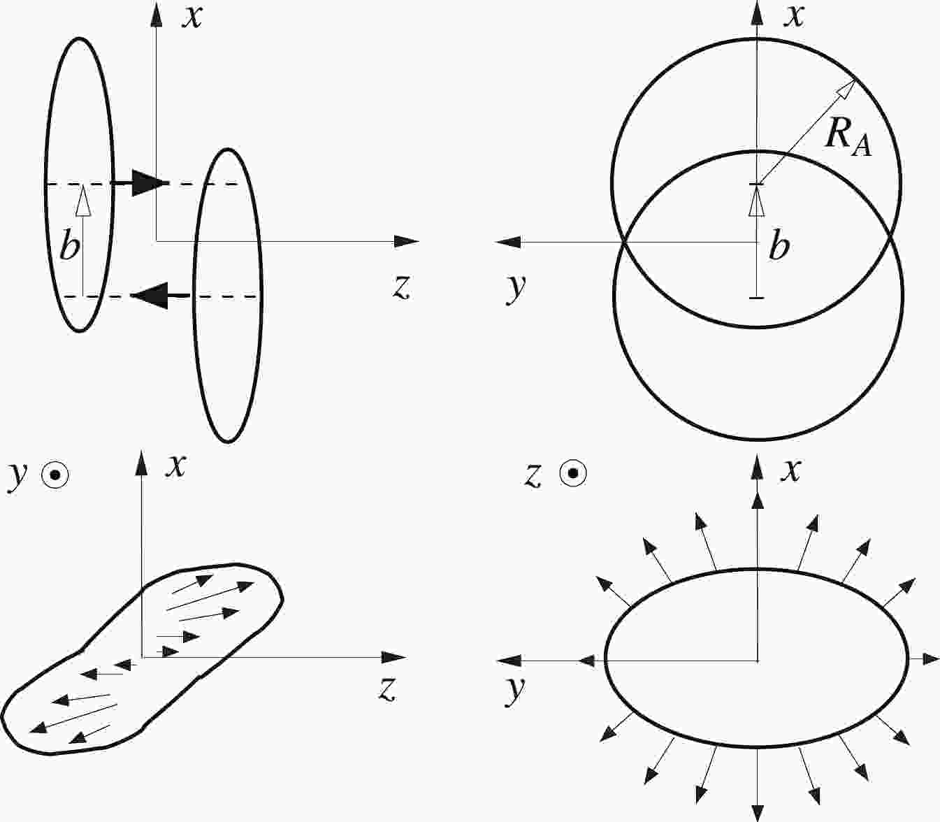
There is an intrinsic rotation of the initially produced matter in the reaction plane in non-central heavy ion collisions. The rotation can be characterized by a tilted local rapidity distribution of produced hadrons toward the projectile and target direction in the transverse plane. We consider non-central collisions of two nuclei
$ {A}+{ A} $ : the first one is regarded as the projectile moving in the$ z $ direction, while the second is regarded as the target moving in the$ -z $ direction; see Fig. 1 for an illustration. The impact parameter is in the direction from the target to the projectile, i.e., in the$ x $ direction. The orbital angular momentum (OAM) is in the direction determined by the vector product of the impact parameter and the projectile momentum,$ {{b}}\times{{p}}_{\rm{proj}} $ which is the$ -y $ direction.
Figure 1. Schematic figure taken from [25] for non-central heavy ion collisions with impact parameter
${{b}}$ pointing in the$x$ direction. The orbital angular momentum is in the$-y$ direction.In the center of the rapidity frame for
$ {{p}}+A $ collisions, the proton has rapidity$ Y_{\rm L} $ and interacts at a transverse impact parameter$ {{r}}_{T} $ with$ N_{\rm{Part}}^{A}\approx\sigma_{NN}T_{A}({{r}}_{T}) $ nucleons with rapidity$ -Y_{\rm L} $ , where$ T_{A}({{r}}_{T}) $ is the thickness function or the number of nucleons per unit area$ T_{A}({{r}}_{T}) = \int {\rm d}z\rho_{A}({{r}}), $

(1) where
$ {{r}} = (x,y,z) $ ,$ {{r}}_{T} = (x,y) $ , and$ \rho_{A} $ is the number density of nucleons in the nucleus,$ \sigma_{NN} $ is the inelastic cross-section of nucleon-nucleon collisions, and$ Y_{\rm L}\approx \ln[\sqrt{s}/(2m_{N})] $ is the largest rapidity. The triangular rapidity distribution of hadrons is the result of string fragmentation between the projectile proton and the target nucleus. The hadrons produced by the wounded projectile proton are in the rapidity range$ Y\in[0,Y_{\rm L}] $ , while those produced by the wounded target nucleons are in the range$ Y\in[-Y_{\rm L},0] $ . The rapidity distribution of produced hadrons is approximately given by the BGK model [26] as$ \frac{{\rm d}^{3}N_{{{p}}A}}{{\rm d}^{2}{{r}}_{T}{\rm d}Y} = \frac{{\rm d}N_{{pp}}}{{\rm d}Y}\left[T_{A}({{r}}_{T})\frac{Y_{\rm L}-Y}{2Y_{\rm L}}+T_{{{p}}}\frac{Y_{\rm L}+Y}{2Y_{\rm L}}\right], $

(2) where
$ T_{{{p}}}\approx1 $ is the number of projectile protons per unit area. In the forward or projectile region$ Y\approx Y_{\rm L} $ , the rapidity distribution approaches that of p+p collisions$ {\rm d}N_{{pp}}/{\rm d}Y $ , while in the backward or target region, it approaches$ ({\rm d}N_{{pp}}/{\rm d}Y)T_{A}({{r}}_{T}) $ . From the experimental data, we take a Gaussian form for$ {\rm d}N_{{pp}}/{\rm d}Y $ ,$ \frac{{\rm d}N_{{pp}}}{{\rm d}Y} = a_{1}\,\exp\left(-\frac{Y^{2}}{a_{2}}\right)\frac{1}{\sqrt{1+a_{3}(\cosh Y)^{4}}}, $

(3) where
$ a_{1} $ ,$ a_{2} $ , and$ a_{3} $ are parameters:$ a_{1} $ sets the magnitude at$ Y = 0 $ , and$ a_{2} $ and$ a_{3} $ describe the width of the rapidity distribution. The values of these parameters in inelastic non-diffractive events for p+p collisions are determined by simulation results using PYTHIA8.2 [29] (see Fig. 2) and are listed in Table 1.$\sqrt{s_{NN}}/{\rm{GeV}}$ 

200 130 62.4 54.4 39 27 19.6 14.5 11.5 7.7 a1 4.584 4.096 3.862 3.726 3.420 3.421 3.099 3.049 2.784 2.831 a2 26.112 25.896 18.911 18.931 18.779 13.555 13.629 9.947 10.488 8.008 a3 $9.70\times10^{-8}$ 

$5.61\times10^{-7}$ 

$9.75\times10^{-6}$ 

$1.71\times10^{-5}$ 

$6.61\times10^{-5}$ 

$2.50\times10^{-4}$ 

$8.76\times10^{-4}$ 

$2.44\times10^{-3}$ 

$5.90\times10^{-3}$ 

$9.40\times10^{-3}$ 

Table 1. Values of parameters in the hadron rapidity distribution in inelastic non-diffractive events for p+p collisions at various collision energies from simulation using PYTHIA8.2 [29].
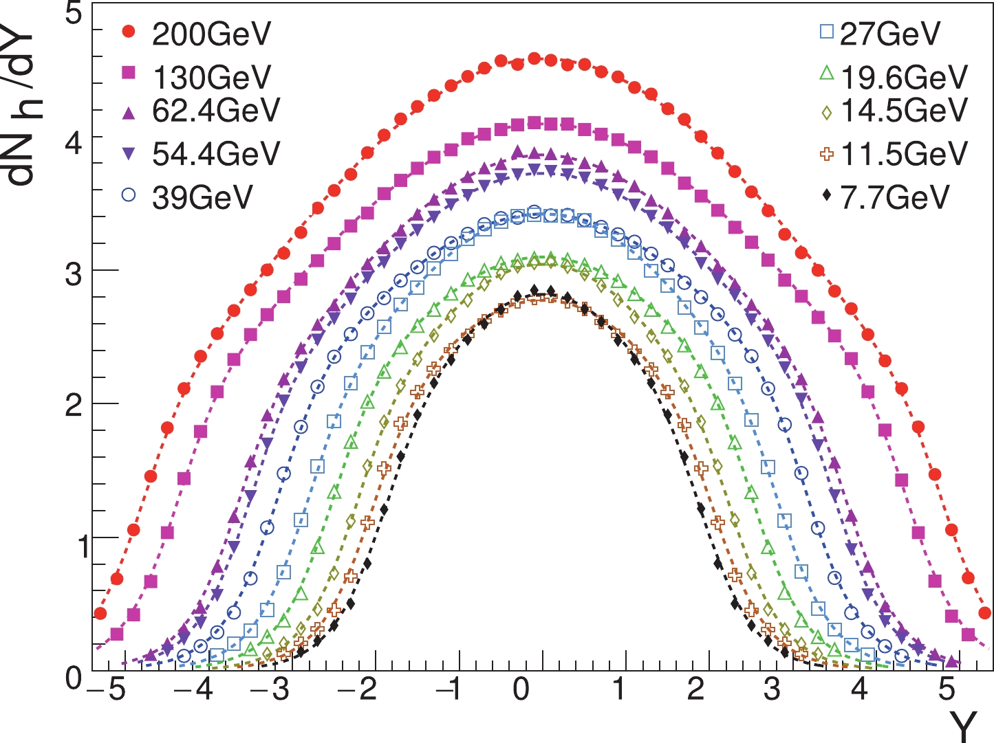
Figure 2. (color online) Simulation results of hadron rapidity distributions in inelastic non-diffractive events for p+p collisions using PYTHIA8.2. The curves of Eq. (3) are shown in lines.
The trapezoidal shape of the rapidity distribution in (2) in the BGK model is a consequence of the string fragmentation and can be described naturally using the LUND string [30] and HIJING model [31, 32]. An extension of the BGK model has been applied to the jet tomography of twisted strongly coupled quark-qluon plasmas [33], as well as the global polarization in nucleus-nucleus collisions [4]. In nucleus-nucleus collisions with projectile
$ A $ and target$ B $ , at the point$ {{r}}_{T} = (x,y) $ in the transverse plane in the participant region (the coordinate system is shown in the upper-left of Fig. 1), the rapidity distribution of produced hadrons has the form that is a generalization of Eq. (2), i.e., the sum over contributions from projectile ('proj') and target ('tar')$ \begin{aligned}[b] \frac{{\rm d}^{3}N_{AB}}{{\rm d}^{2}{{r}}_{T}{\rm d}Y} =& \frac{{\rm d}^{3}N_{A}^{\rm{proj}}}{{\rm d}^{2}{{r}}_{T}{\rm d}Y}+\frac{{\rm d}^{3}N_{B}^{\rm{tar}}}{{\rm d}^{2}{{r}}_{T}{\rm d}Y} \\ =& \frac{{\rm d}N_{{pp}}}{{\rm d}Y}\left[T_{A}({{r}}_{T}-{{b}}/2)\frac{Y_{\rm L}+Y}{2Y_{\rm L}}+T_{B}({{r}}_{T}+{{b}}/2)\frac{Y_{\rm L}-Y}{2Y_{\rm L}}\right]. \end{aligned} $

(4) Here, thickness functions
$ T_{A}({{r}}_{T}-{{b}}/2) $ and$ T_{B}({{r}}_{T}+{{b}}/2) $ in Eq. (4) are given by$ T_{A,B}({{r}}_{T}\mp{{b}}/2) = \int {\rm d}z\rho^{A,B}({{r}}_{T}\mp{{b}}/2), $

(5) where
$ \rho^{A,B}({{r}}_{T}\mp{{b}}/2) $ are the participant nucleon number density functions of nuclei$ A $ and$ B $ . One can verify that distribution (4) is proportional to$ T_{A/B}({{r}}_{T}\mp{{b}}/2) $ at$ Y = \pm Y_{\rm L} $ .From Eq. (4), we can derive the distribution in the in-plane position
$ x $ and the rapidity$ Y $ by integrating over the out-plane position$ y $ in the range$ [-y_{m},y_{m}] $ ,$\begin{aligned}[b]\!\!\! \frac{{\rm d}^{2}N_{AB}}{{\rm d}x{\rm d}Y} =& \frac{{\rm d}N_{{pp}}}{{\rm d}Y}\left\{ \frac{1}{2}\int_{-y_{m}}^{y_{m}}{\rm d}y\left[T_{A}({{r}}_{T}-{{b}}/2)+T_{B}({{r}}_{T}+{{b}}/2)\right]\right. \\ &\left.+\frac{Y}{2Y_{\rm L}}\int_{-y_{m}}^{y_{m}}{\rm d}y\left[T_{A}({{r}}_{T}-{{b}}/2)-T_{B}({{r}}_{T}+{{b}}/2)\right]\right\} , \end{aligned} $

(6) where
$ y_{m} $ is the maximum of$ y $ at a specific$ x $ ; in the hard sphere model of the nuclear density distribution, it is defined by the boundary of the overlapping region of two nuclei, while in the Woods-Saxon model, there is no sharp boundary, but it can be set to a value much larger than$ y_{m} $ in the hard sphere model. We define the normalized probability distribution of$ Y $ at$ x $ ,$ f(Y,x) = \left(\frac{{\rm d}N_{AB}}{{\rm d}x}\right)^{-1}\frac{{\rm d}^{2}N_{AB}}{{\rm d}x{\rm d}Y}, $

(7) where the distribution
$ {\rm d}N_{AB}/{\rm d}x $ is given by$ \begin{aligned} \frac{{\rm d}N_{AB}}{{\rm d}x} =& \int_{-Y_{\rm L}}^{Y_{\rm L}}{\rm d}Y\frac{{\rm d}^{2}N_{AB}}{{\rm d}x{\rm d}Y} \\ =& \int_{0}^{Y_{\rm L}}{\rm d}Y\frac{{\rm d}N_{{pp}}}{{\rm d}Y}\int_{-y_{m}}^{y_{m}}{\rm d}y\left[T_{B}({{r}}_{T}+{{b}}/2)+T_{A}({{r}}_{T}-{{b}}/2)\right]. \end{aligned} $

(8) According to the Bjorken scaling model [25], the average rapidity of the particle as a function of
$ Y $ at$ x $ in the rapidity window$ [Y-\Delta_{Y}/2,Y+\Delta_{Y}/2] $ is given by$ \begin{aligned}[b]\left\langle Y\right\rangle _{\Delta} = \frac{\displaystyle\int_{Y-\Delta_{Y}/2}^{Y+\Delta_{Y}/2}{\rm d}Y^{\prime}\:Y^{\prime}f(Y^{\prime},x)}{\displaystyle\int_{Y-\Delta_{Y}/2}^{Y+\Delta_{Y}/2}{\rm d}Y^{\prime}\:f(Y^{\prime},x)} \approx Y+\frac{\Delta_{Y}^{2}}{12}\frac{1}{f(Y,x)}\frac{{\rm d}f(Y,x)}{{\rm d}Y}, \end{aligned} $

(9) where
$ \Delta_{Y} $ is the width of the rapidity window in which particles interact to reach collectivity. We assumed$ \Delta_{Y}\ll Y $ so that$ \Delta_{Y} $ can be treated as a perturbation. The average rapidity of the particle as a function of$ x $ in the full rapidity range reads$ \begin{aligned}[b]\left\langle Y\right\rangle =& \frac{\displaystyle\int_{-Y_{\rm L}}^{Y_{\rm L}}{\rm d}Y\:Yf(Y,x)}{\displaystyle\int_{-Y_{\rm L}}^{Y_{\rm L}}{\rm d}Y\:f(Y,x)} \\ =& \frac{1}{Y_{\rm L}}\left\langle Y^{2}\right\rangle _{{pp}}\frac{\displaystyle\int_{-y_{m}}^{y_{m}}{\rm d}y\left[T_{A}({{r}}_{T}-{{b}}/2)-T_{B}({{r}}_{T}+{{b}}/2)\right]}{\displaystyle\int_{-y_{m}}^{y_{m}}{\rm d}y\left[T_{A}({{r}}_{T}-{{b}}/2)+T_{B}({{r}}_{T}+{{b}}/2)\right]}, \end{aligned} $

(10) where
$ \left\langle Y^{2}\right\rangle _{{pp}} $ is defined as$ \begin{aligned} \left\langle Y^{2}\right\rangle _{{pp}} = \frac{\displaystyle\int_{-Y_{\rm L}}^{Y_{\rm L}}{\rm d}Y\:({\rm d}N_{{pp}}/{\rm d}Y)Y^{2}}{\displaystyle\int_{-Y_{\rm L}}^{Y_{\rm L}}{\rm d}Y\:({\rm d}N_{{pp}}/{\rm d}Y)}. \end{aligned} $

(11) The average longitudinal momentum
$ p_{z} $ and the average energy$ E_{p} $ of the particle are$ \begin{aligned}[b] \left\langle p_{z}\right\rangle = & \left\langle p_{T}\right\rangle \sinh\left\langle Y\right\rangle _{\Delta} \\ \approx & \left\langle p_{T}\right\rangle \sinh Y+\left\langle p_{T}\right\rangle \frac{\Delta_{Y}^{2}}{12}\frac{{\rm d}\ln f(Y,x)}{{\rm d}Y}\cosh Y, \end{aligned} $

$ \begin{aligned}[b] \left\langle E_{p}\right\rangle = & \left\langle p_{T}\right\rangle \cosh\left\langle Y\right\rangle _{\Delta} \\ \approx & \left\langle p_{T}\right\rangle \cosh Y+\left\langle p_{T}\right\rangle \frac{\Delta_{Y}^{2}}{12}\frac{{\rm d}\ln f(Y,x)}{{\rm d}Y}\sinh Y, \end{aligned} $

(12) where we have treated terms proportional to
$ \Delta_{Y}^{2} $ as a perturbation. At a given$ Y $ , we consider two particles located at$ x+\Delta x/2 $ and$ x-\Delta x/2 $ . In their center of mass frame, the local average OAM for two colliding particles is given by [25]$ \begin{aligned}[b] \left\langle L_{y}\right\rangle \approx &-(\Delta x)\left\langle p_{z}^{\rm{cm}}\right\rangle \\ \approx & -(\Delta x)^{2}\left\langle p_{T}\right\rangle \frac{\Delta_{Y}^{2}}{24}\frac{{\rm d}\ln f(Y,x)}{{\rm d}Y{\rm d}x}, \end{aligned} $

(13) where
$ \left\langle p_{z}^{\rm{cm}}\right\rangle $ is the average longitudinal momentum in the center of mass frame for one particle. Here,$ \Delta x $ is a typical impact parameter of particle scatterings, and the function${\rm d}\ln f(Y,x)/{\rm d}x{\rm d}Y $ is called the shear of longitudinal momentum (SLM). In the following sections, we will use the average SLM over the in-plane coordinate$ \left\langle \frac{{\rm d}\ln f(Y,x)}{{\rm d}Y{\rm d}x}\right\rangle _{x} = \frac{\displaystyle\int {\rm d}x({\rm d}N_{AB}/{\rm d}x{\rm d}Y)({\rm d}\ln f(Y,x)/{\rm d}Y{\rm d}x)}{\displaystyle\int {\rm d}x({\rm d}N_{AB}/{\rm d}x{\rm d}Y)}, $

(14) where
$ {\rm d}N_{AB}/{\rm d}x{\rm d}Y $ is given in Eq. (6) as a weight function. -
In this section, we will calculate the rapidity distributions for hadrons
$ f(Y,x) $ in Eq. (7) with the hard sphere (HS) and Woods-Saxon (WS) nuclear density distributions, which are involved in the thickness functions in Eq. (5). As a simple illustration, we consider collisions of two identical nuclei with nucleon number$ A $ . -
The HS nuclear density is given by
$ \rho_{\rm{HS}}({{r}}) = \frac{3A}{4\pi R_{A}^{3}}\theta(R_{A}-r), $

(15) where
$ R_{A} = 1.2A^{1/3} $ fm is the radius of the nucleus. The thickness functions have the analytical form$ T_{A}({{r}}_{T}\pm{{b}}/2) = \frac{6A}{4\pi R_{A}^{3}}\left[R_{A}^{2}-(x\pm b/2)^{2}-y^{2}\right]^{1/2}. $

(16) Inserting the above into Eq. (4), we obtain the hadron distribution
$ {\rm d}N_{AA}/({\rm d}x{\rm d}y{\rm d}Y) $ , whose numerical results are shown in Fig. 3 at three rapidity values in Au+Au collisions at$ \sqrt{s_{NN}} = 200 $ GeV with the impact parameter$ b = 1.2R_{A} $ . In the HS model, the overlapping region of two nuclei is limited by$ |x|\!<\!R_{A}\!-\!b/2 $ and$ |y|\!<\!\sqrt{R_{A}^{2}\!-\!(|x|\!+\!b/2)^{2}} $ . We see that the distribution at$ Y = 0 $ is symmetric in$ x $ and$ y $ , while the distribution in the forward (backward) rapidity is shifted to the right (left) in the$ x $ direction.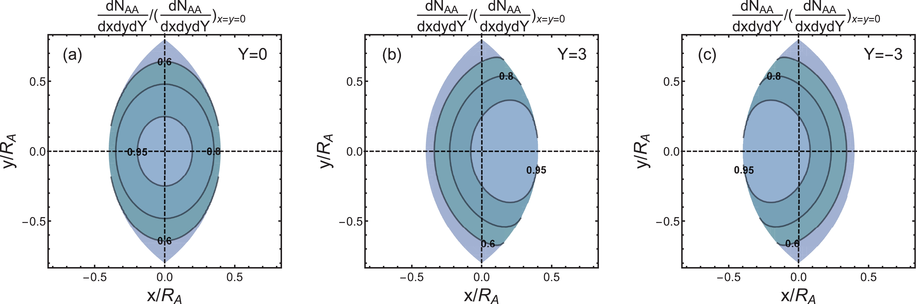
Figure 3. (color online) Hadron distributions (contour plot) in the HS model in the transverse plane for Au+Au collisions at
$\sqrt{s_{NN}} = 200$ GeV and$b = 1.2R_{A}$ . The number on the contour line denotes the value on the line normalized by that at the origin. The rapidity values are chosen to be (a)$Y = 0$ (central), (b)$Y = 3$ (forward), and (c)$Y = -3$ (backward).Integrating over the out-plane coordinate
$ y $ , we obtain the hadron distribution function$ \frac{{\rm d}^{2}N_{AA}}{{\rm d}x{\rm d}Y} = \frac{6A}{4\pi R_{A}^{3}}\frac{{\rm d}N_{pp}}{{\rm d}Y}\left[C_{1}^{+}+C_{1}^{-}+\frac{Y}{Y_{\rm L}}\left(C_{1}^{+}-C_{1}^{-}\right)\right], $

(17) where
$ C_{1}^{\pm} $ are defined in Eq. (27). In Fig. 4(a), we show$ {\rm d}N_{AA}/{\rm d}x{\rm d}Y $ as functions of the in-plane coordinate$ x $ at various rapidity values. We see that the distribution at$ Y = 0 $ is symmetric, while the distribution at forward (backward) rapidity is shifted to the positive (negative)$ x $ . The magnitude of the shift increases slightly with the rapidity. In Fig. 4(b), we show$ {\rm d}N_{AA}/{\rm d}x{\rm d}Y $ as functions of the rapidity for various values of$ x $ . We see that the distribution at$ x = 0 $ is symmetric, while that at positive (negative)$ x $ is tilted to the forward (backward) rapidity. From Eq. (7), we obtain the normalized function$ f(Y,x) $ as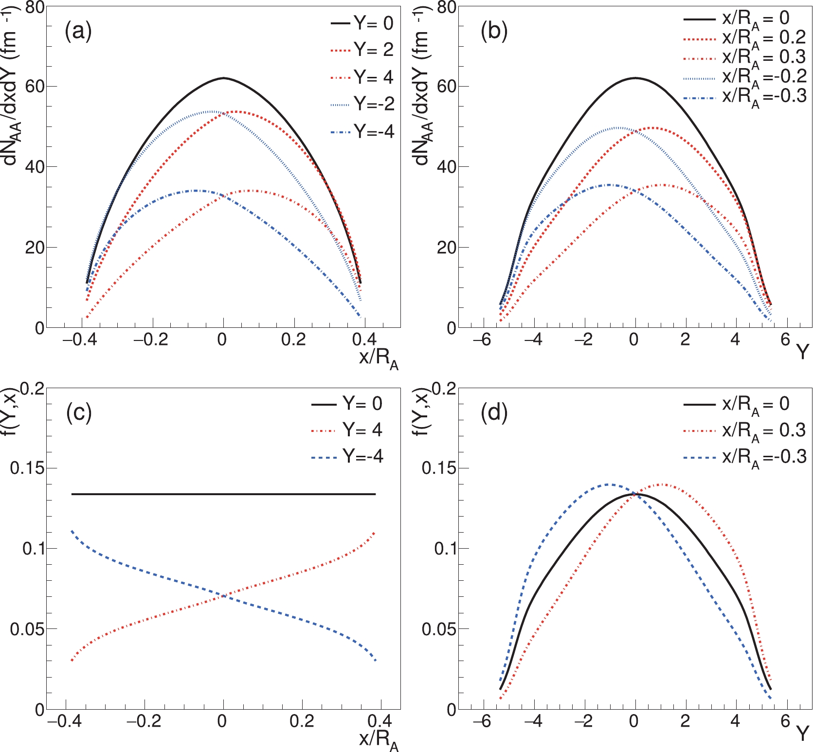
Figure 4. (color online) Hadron distributions in the HS model in Au+Au collisions at
$\sqrt{s_{NN}} = 200$ GeV as functions of (a) the in-plane position$x$ at different rapidity values and as functions of (b) the rapidity$Y$ at different values of$x$ . The impact parameter is set to$b = 1.2R_{A}$ . (c) The normalized distribution$f(Y,x)$ as functions of$x$ at different$Y$ . (d) The normalized distribution$f(Y,x)$ corresponding to (b). The definition of$f(Y,x)$ is given in Eq. (18).$ f(Y,x) = \frac{{\rm d}N_{{pp}}/{\rm d}Y}{2\int_{0}^{Y_{\rm L}}{\rm d}Y({\rm d}N_{{pp}}/{\rm d}Y)}\left(1+\frac{Y}{Y_{\rm L}}\cdot\frac{C_{1}^{+}-C_{1}^{-}}{C_{1}^{+}+C_{1}^{-}}\right), $

(18) where
$ |x|\leqslant R_{A}-b/2 $ and$ b\leqslant 2R_{A} $ . The numeical results of$ f(Y,x) $ are shown in Fig. 4(c, d).The derivative of
$ \ln f(Y,x) $ with respect to$ Y $ and$ x $ is derived in Eq. (37), from which one can obtain the average SLM through Eq. (14). We show numerical results of the average SLM in Fig. 5 as rapidity functions in Au+Au collisions at various collision energies. The average SLM increases slowly with the rapidity via the$ Y/Y_{\rm L} $ term, which can be seen in Eq. (37). The energy dependence of the average SLM is mostly controlled by$ Y_{\rm L}\approx \ln[\sqrt{s}/ (2m_{N})] $ , as shown in Eq. (37). The relatively obvious increase in the forward rapidity region is an artifact of the HS model in comparison with the WS model in the next subsection. The reason for this is that there is a sharp decrease in the nucleon density at the nucleus boundary in the HS model, which gives an infinite derivative in the SLM in the forward rapidity region. In the WS model, however, the decrease in the nucleon density at the boundary is smooth, resulting in a mild increase in the average SLM.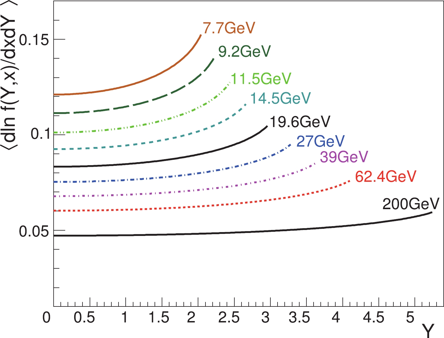
Figure 5. (color online) Average SLM as functions of the rapidity
$Y$ in the HS model for Au+Au collisions at various collision energies. The impact parameter is set to$b = 1.2R_{A}$ . The cutoff in$Y$ at a collision energy is set to$0.9Y_{\rm L}$ .From Eq. (10), we obtain the average rapidity in the full rapidity range as
$ \left\langle Y\right\rangle = \frac{1}{Y_{\rm L}}\left\langle Y^{2}\right\rangle _{{pp}}\frac{C_{1}^{+}-C_{1}^{-}}{C_{1}^{+}+C_{1}^{-}}. $

(19) The numerical result of the above average rapidity is shown in Fig. 6. The result for
$ \left\langle Y\right\rangle $ in the WS model in the next subsection (see Fig. 10) is similar to the result of Eq. (19) or Fig. 6, except in the boundary region. Comparison with the result of Ref. [25] is also made in Fig. 10.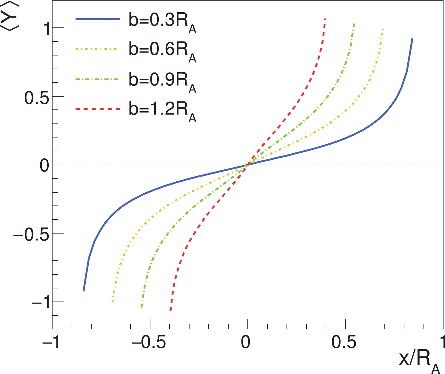
Figure 6. (color online) Average rapidity in the full rapidity range for Au+Au collisions at
$\sqrt{s_{NN}} = 200$ GeV as functions of$x$ from Eq. (19) in the HS model. -
In this subsection, we choose a more realistic nuclear density distribution, the WS distribution, defined as
$ f_{\rm{WS}}({{r}}) = \frac{C_{0}}{\exp\left[\left(r-R_{A}\right)/a\right]+1}, $

(20) where
$ r = |{{r}}| $ ,$ a = 0.54 $ fm, and$ C_{0} $ is a normalization constant to make the volume integral of$ f_{\rm{WS}}({{r}}) $ equal to the number of nucleons in the nucleus,$ C_{0} = \frac{A}{4\pi}\left[\int_{0}^{\infty}{\rm d}rr^{2}\frac{1}{\exp[(r-R_{A})/a]+1}\right]^{-1}. $

(21) For Au-197 nuclei, we have
$ R_{A}\approx6.98 $ fm and$ C_{0}\approx A/(4\pi)/120.2\approx0.131\:{\rm{fm}}^{-3} $ . According to the Glauber model, the participant nucleon number density for two colliding nuclei is given by$ \begin{aligned}[b]\rho_{\rm{WS}}^{A,B}({{r}}_{T}\mp{{b}}/2) =& f_{\rm{WS}}^{A,B}({{r}}_{T}\mp{{b}}/2)\\&\times\left\{ 1-\exp\left[-\sigma_{NN}\int {\rm d}zf_{\rm{WS}}^{B,A}({{r}}_{T}\pm{{b}}/2)\right]\right\}, \end{aligned} $

(22) where
$ \sigma_{NN} $ can be taken as the inelastic pp collision cross-section.We consider collisions of two identical nuclei. With the WS distribution in Eq. (20), we can calculate
$ f(Y,x) $ in Eq. (7). From Eq. (5), the thickness function becomes$ \begin{aligned}[b] T_{A}({{r}}_{T}\pm{{b}}/2) =& \int_{-\infty}^{\infty}{\rm d}z\rho_{\rm{WS}}^{A}({{r}}_{T}\pm{{b}}/2) \\ =& \int_{-\infty}^{\infty}{\rm d}zf_{\rm{WS}}({{r}}_{T}\pm{{b}}/2)\\&\times \left\{ 1-\exp\left[-\sigma_{NN}\int {\rm d}zf_{\rm{WS}}({{r}}_{T}\mp{{b}}/2)\right]\right\}. \end{aligned} $

(23) Substituting Eq. (23) into Eqs. (4) and (6), we obtain the hadron distribution
$ {\rm d}N_{AA}/({\rm d}x{\rm d}y{\rm d}Y) $ in the$ xy $ plane and$ {\rm d}N_{AA}/({\rm d}x{\rm d}Y) $ by an integration over$ y $ , respectively. The numerical results for$ {\rm d}N_{AA}/({\rm d}x{\rm d}y{\rm d}Y) $ and$ {\rm d}N_{AA}/({\rm d}x{\rm d}Y) $ are shown in Figs. 7 and 8, respectively for different rapidity values in Au+Au collisions at 200 GeV with$ b = 1.2R_{A} $ . Similar to the results of the HS model in Figs. 3 and 4, in the forward/backward rapidity region, the hadron distributions are tilted toward the positive/negative$ x $ . However, different from the results of the HS model, the hadron distributions in the WS model are smooth at the edge of the overlapping region.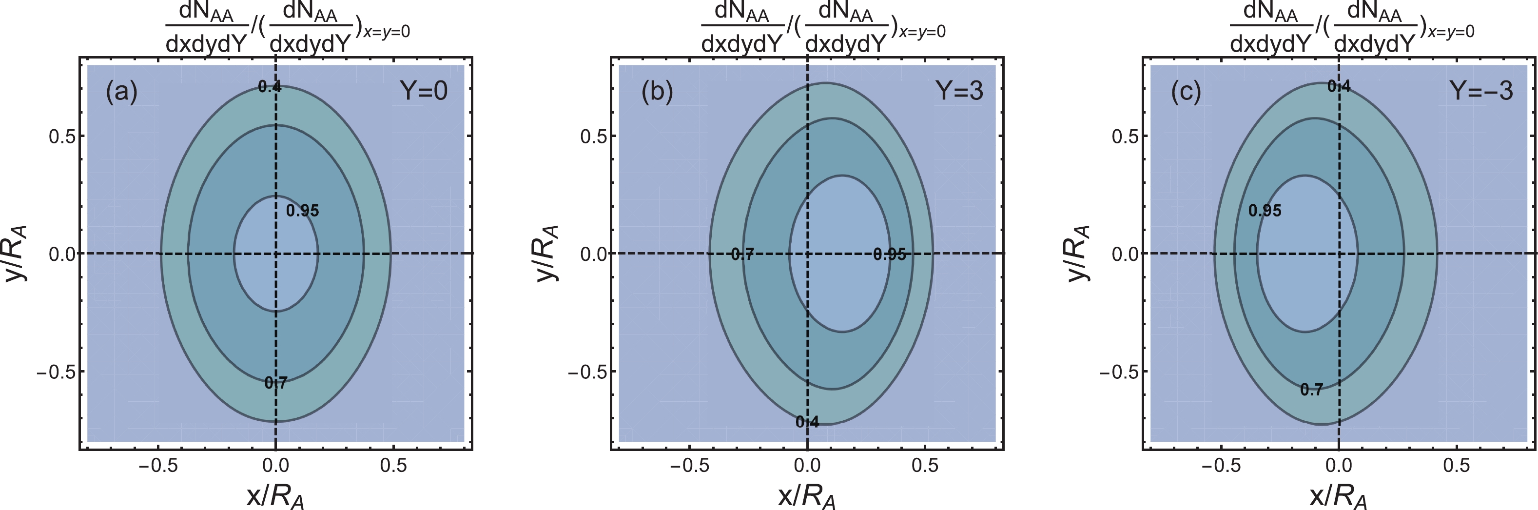
Figure 7. (color online) Hadron distributions (contour plot) in the WS model in the transverse plane for Au+Au collisions at
$\sqrt{s_{NN}} = 200$ GeV and$b = 1.2R_{A}$ . The number on the contour line denotes the value on the line normalized by that at the origin. The rapidity values are chosen to be (a)$Y = 0$ (central), (b)$Y = 3$ (forward), and (c)$Y = -3$ (backward).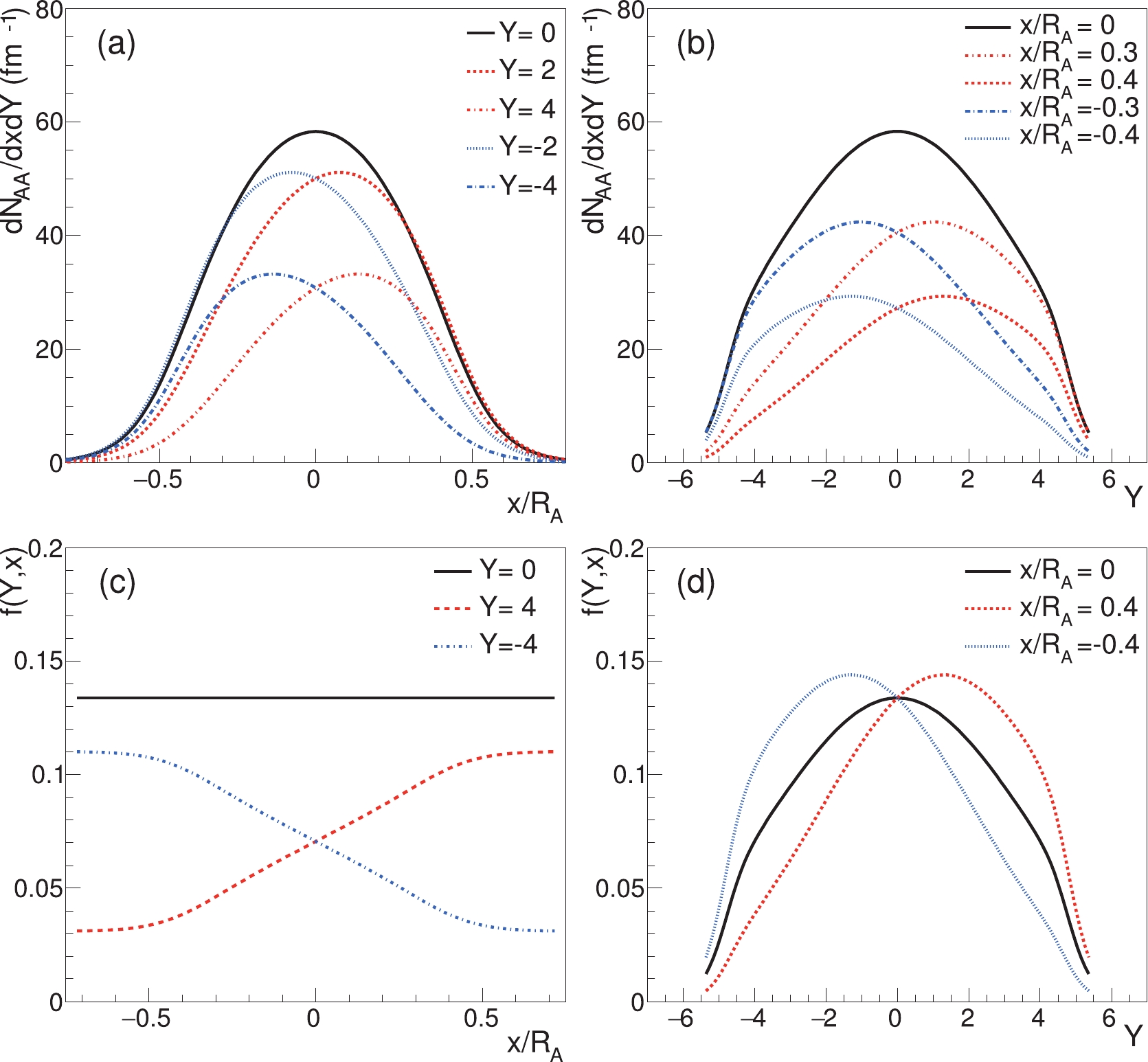
Figure 8. (color online) Hadron distributions in the WS model in Au+Au collisions at
$\sqrt{s_{NN}} = 200$ GeV as functions of (a) the in-plane position$x$ at different rapidity values and as functions of (b) the rapidity$Y$ at different values of$x$ . The impact parameter is set to$b = 1.2R_{A}$ . (c) The normalized distribution$f(Y,x)$ as functions of$x$ at different$Y$ . (d) The normalized distribution$f(Y,x)$ corresponding to (b). The definition of$f(Y,x)$ is given in Eq. (7).In Fig. 9, we show numerical results for the average SLM, applying Eq. (14) to the WS model. We choose
$ b = 1.2R_{A} $ in Au+Au collisions at different collision energies. We choose$ \sigma_{NN} $ as the inelastic proton-proton cross-section determined by the global fit of the experimental data [34], whose values are listed in Table 2. Also shown in Table 2 are the values of the average SLM at$ Y = 0 $ in Au+Au collisions with the HS and WS distributions.$\sqrt{s_{NN}}$ /GeV

200 62.4 54.4 39 27 19.6 14.5 11.5 9.2 7.7 $\sigma_{NN}$ /mb

42.0 36.3 35.2 33.6 32.8 32.3 31.8 31.4 30.9 30.6 $\left\langle \frac{{\rm d}\ln f(Y,x)}{{\rm d}Y{\rm d}x}\right\rangle _{x,{\rm{HS}}}$ 

0.0471 0.0602 0.0622 0.0678 0.0753 0.0833 0.0925 0.101 0.111 0.121 $\left\langle \frac{{\rm d}\ln f(Y,x)}{{\rm d}Y{\rm d}x}\right\rangle _{x,{\rm{WS}}}$ 

0.0374 0.0460 0.0472 0.0507 0.0558 0.0614 0.0678 0.0739 0.0809 0.0876 Table 2. Inelastic nucleon-nucleon cross-section
$\sigma_{NN}$ at different collisions energies (first two rows). The numerical results of the average SLM at$Y = 0$ in Au+Au collisions at different collisions energies (last two rows). The impact parameter is set to$b = 1.2R_{A}$ corresponding to 20%-50% centrality in experiments.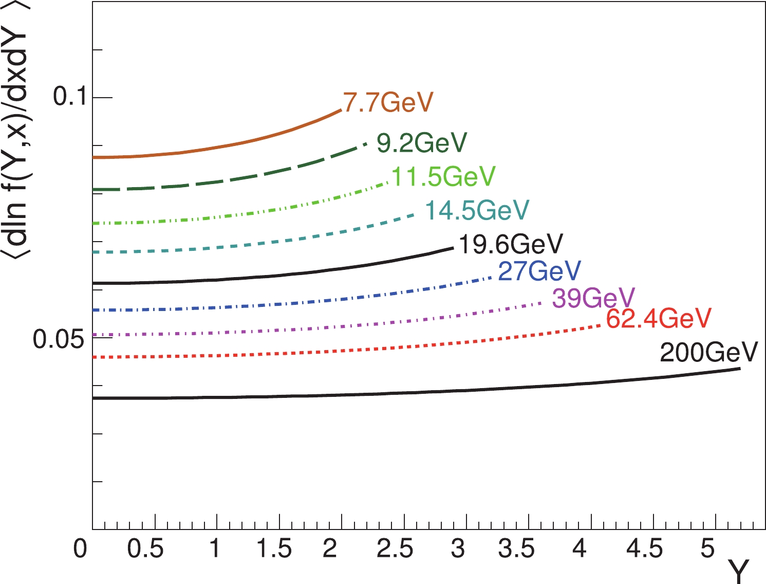
Figure 9. (color online) Average SLM as functions of the rapidity
$Y$ in the WS model for Au+Au collisions at various collision energies. The impact parameter is set to$b = 1.2R_{A}$ . The cutoff in$Y$ at a collision energy is set to$0.9Y_{\rm L}$ .Similar to the results of the HS model, the average SLM at
$ Y = 0 $ increases with decreasing collision energies, and it is a slowly increasing function of$ Y $ . There are also some differences between the WS and HS results. First, because of the smooth function in the WS model at the edge of the nucleus, the rapidity dependence of the average SLM in the WS model is slightly weaker than that in the HS model. Second, in addition to the explicit collision energy dependence of$ Y_{\rm L} $ ,$ \sigma_{NN} $ also depends on the collision energy and enters the thickness function via Eq. (22); therefore, the increase in the average SLM at$ Y = 0 $ in the WS model with decreasing collision energy is slightly slower than in the HS model.The numerical result for the average rapidity in the full rapidity range from Eq. (10) is shown in Fig. 10. In the figure, the result of Fig. 5 at
$ b = 0.6R_{A} $ in Ref. [25] is also shown for comparison. The strong fluctuations at the edge in the simulation result of Ref. [25] are due to the small number of nucleons in the boundary region. The difference between Fig. 10 with the WS distribution and Fig. 6 with the HS distribution is that the edge of the overlapping region of two nuclei$ \left\langle Y\right\rangle $ with the WS distribution is smoothly vanishing far outside the overlapping region, but$ \left\langle Y\right\rangle $ with the HS distribution is discontinuous at the boundary.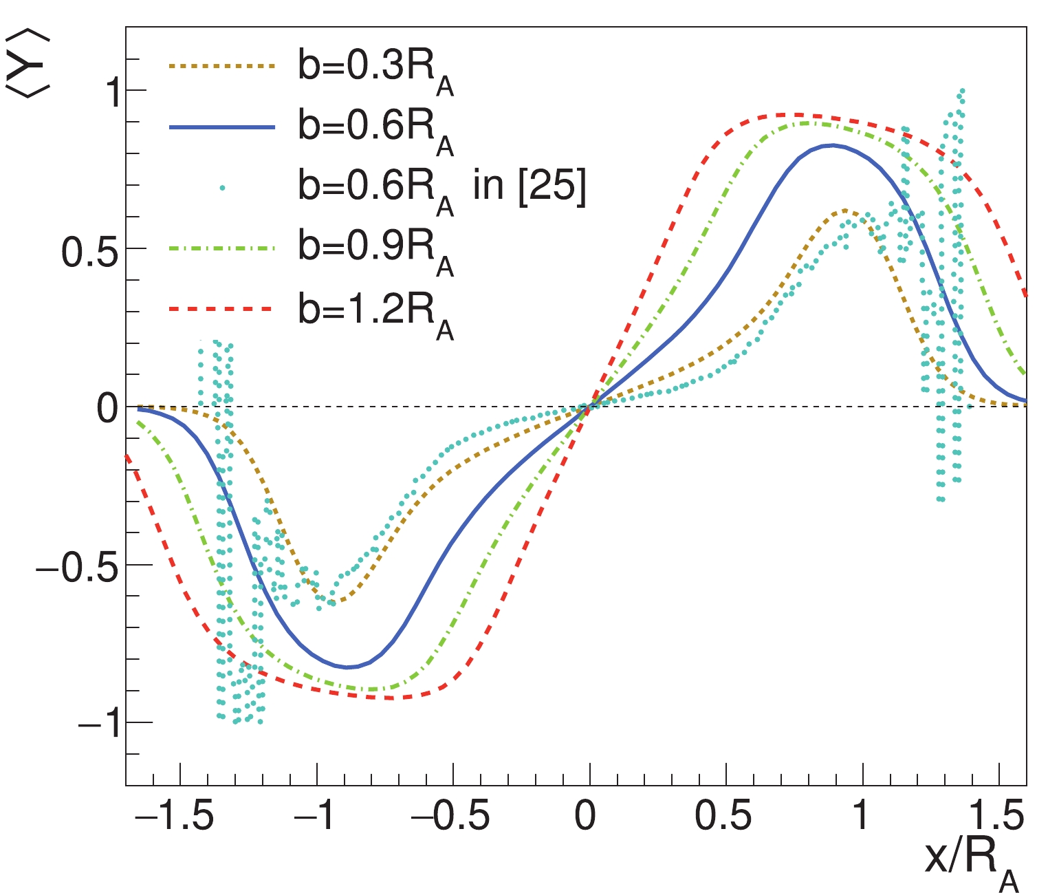
Figure 10. (color online) Average rapidity in the full rapidity range for Au+Au collisions
$\sqrt{s_{NN}} = 200$ GeV as a function of$x$ from Eq. (10) in the WS model. -
As proposed in [25], the OAM in peripheral collisions of two nuclei can induce hadron polarization. Here, we assume that the polarization is proportional to the local OAM
$ \begin{aligned} P_{q}\left(Y\right) = \alpha(Y)\left\langle L_{y}\right\rangle = -\alpha(Y)(\Delta x)^{2}\frac{\Delta_{Y}^{2}}{24}\left\langle p_{T}\right\rangle \left\langle \frac{{\rm d}\ln f(Y,x)}{{\rm d}Y{\rm d}x}\right\rangle _{x}, \end{aligned} $

(24) where we have replaced the SLM in Eq. (13) with its average in Eq. (14), and
$ \alpha(Y) $ is a rapidity-dependent coefficient. The minus sign means that the polarization is along the$ -y $ direction. We define a parameter$ \kappa(Y) = \alpha(Y)(\Delta x)^{2}\Delta_{Y}^{2}, $

(25) as a function of
$ Y $ . Note that in principle$ \Delta x $ ,$ \Delta_{Y} $ , and$ \left\langle p_{T}\right\rangle $ can also depend on$ Y $ .The global polarization of
$ \Lambda $ hyperons at mid-rapidity has been measured in the STAR experiment, by which the parameters in Eq. (24) can be determined. At mid-rapidity$ Y = 0 $ , Eq. (24) becomes$ P_{q}(Y = 0) = -\frac{1}{24}\kappa_{0}\left\langle p_{T}\right\rangle \left\langle \frac{{\rm d}\ln f(Y,x)}{{\rm d}Y{\rm d}x}\right\rangle _{x,Y = 0}, $

(26) where we have combined three parameters into one,
$ \kappa_{0}\equiv\kappa(Y = 0) $ . The average transverse momentum$ \left\langle p_{T}\right\rangle $ as a function of the rapidity and collision energy can be fitted using available data for Kaons; see Appendix C. Results of the average SLM at$ Y = 0 $ are already shown in Table 2.As our first option, we assume that the parameter
$ \kappa_{0} $ is a constant of the collision energy, whose value is chosen to describe via Eq. (26) the polarization data in the energy range of 7.7-62.4 GeV. The results are shown in the left panel of Fig. 11. We see that the collision energy dependence of$ P_{q}(Y = 0) $ in HS with$ \kappa_{0} = 6.4 $ and that in WS with$ \kappa_{0} = 8.4 $ are roughly consistent with the polarization data in the energy range of 7.7-62.4 GeV, but not consistent with the data at 200 GeV. Interestingly, we find that the energy dependence of our results in both the HS and WS models can be well fitted by$ 1/Y_{\rm L} $ behavior, but as in both the HS and WS models, it fails to describe the data at 200 GeV. The reason why we look at such a behavior is because there is a prefactor$ 1/Y_{\rm L} $ in the SLM, as shown in Eq. (37), while the rest of the SLM depends weakly on collision energies. As our second option, we use the energy-dependent$ \kappa_{0} $ to fit the data in the energy range of 7.7-62.4 GeV, including 200 GeV. The results are shown in the right panel of Fig. 11. We will choose the energy-dependent$ \kappa_{0} $ to calculate the rapidity dependence of the global polarization of$ \Lambda $ hyperons.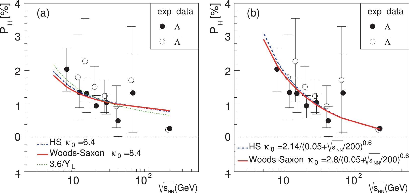
Figure 11. (color online) Global polarization of
$\Lambda$ and$\overline{\Lambda}$ at mid-rapidity in the HS and WS models in Au+Au collisions at different collision energies. The impact parameter is set to$b = 1.2R_{A}$ , corresponding to a centrality of 20%-50%. The STAR data are represented by the solid ($\Lambda$ ) and open ($\overline{\Lambda}$ ) circles [13, 14]. (a)$\kappa_{0}$ is a contant of the collision energy. (b)$\kappa_{0}$ depends on the collision energy.As a test of the model, we calculate the global
$ \Lambda $ polarization at 200 GeV as a function of centralities and compare it with the STAR data [14]. We use the value of$ \kappa_{0} $ at 200 GeV and a centrality of 20%-50%. The values of$ \left\langle p_{T}\right\rangle $ also depend on the centralities and are determined by Table 7 in Ref. [35]. The correspondence between the impact parameter and the centrality is given by Table 2 in Ref. [35]. Then, the main source of the centrality dependence of the global$ \Lambda $ polarization is the average SLM. The calculated result is shown in Fig. 12. We see that the theoretical result increases with the centralities and agrees with the data very well. We also see that in most central collisions, the global polarization vanishes, which indicates a vanishing SLM [1].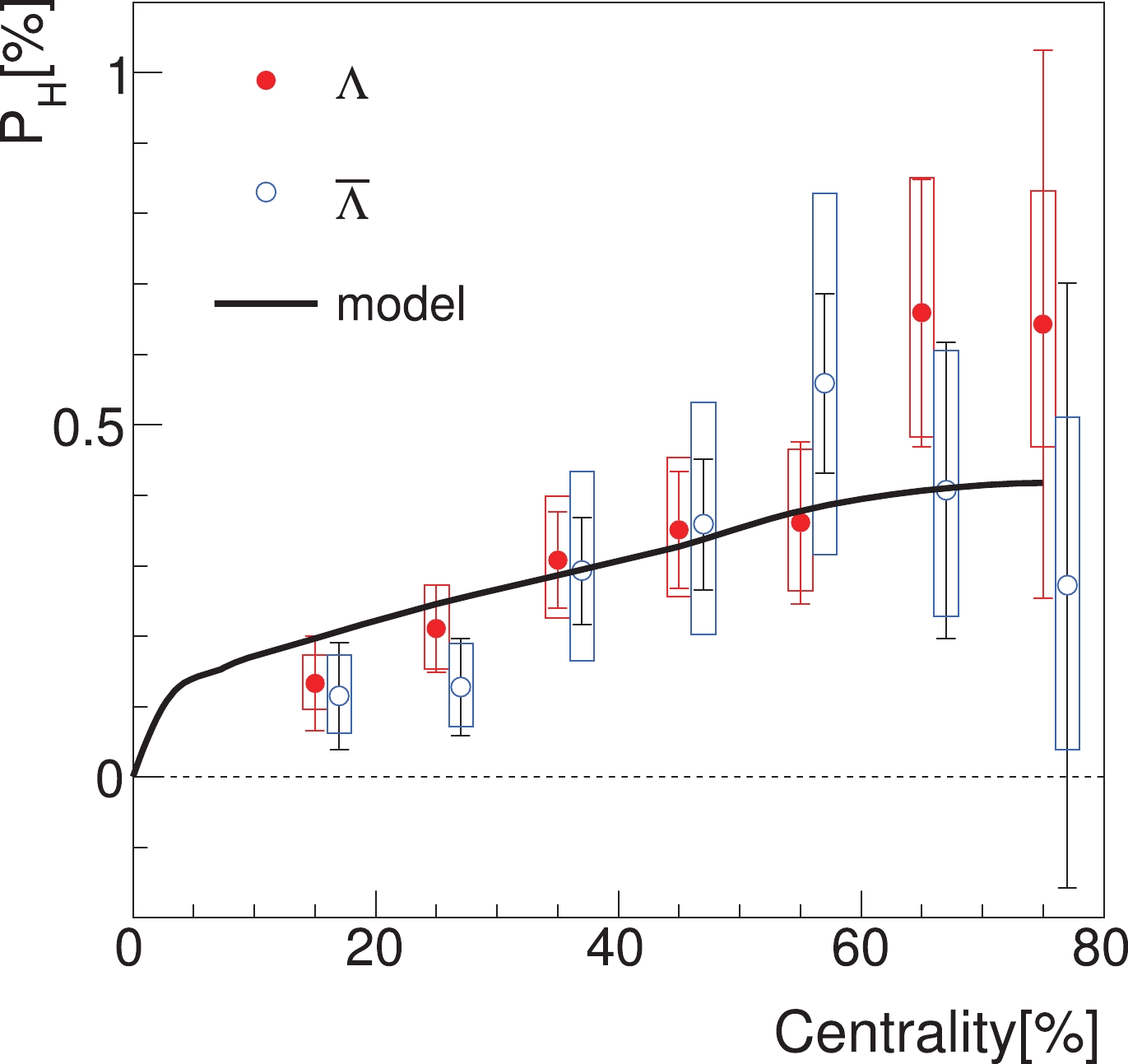
Figure 12. (color online) Global
$\Lambda$ polarization as a function of centralities in comparison with the STAR data [14].Once the values of
$ \kappa_{0} $ are constrained by the polarization data at mid-rapidity, we can predict the polarization of$ \Lambda $ hyperons at a larger rapidity. In our prediction, we use the WS model and the energy-dependent$ \kappa_{0} $ , as determined in the right panel of Fig. 11. Because we do not know the exact rapidity dependence of$ \kappa(Y) $ and$ \left\langle p_{T}\right\rangle $ , we will consider four cases and make corresponding predictions for the rapidity dependence of the global polarization:(a) Both
$ \kappa(Y) = \kappa_{0} $ and$ \left\langle p_{T}\right\rangle $ are taken to be constants in rapidity. Therefore, the rapidity dependence of the global polarization comes solely from the average SLM. This result is shown in Fig. 13(a). We see that the polarization increases slighly with$ Y $ at each collision energy. The positive slope in rapidity (the increase rate of the polarization per unit rapidity) decreases with the collision energy.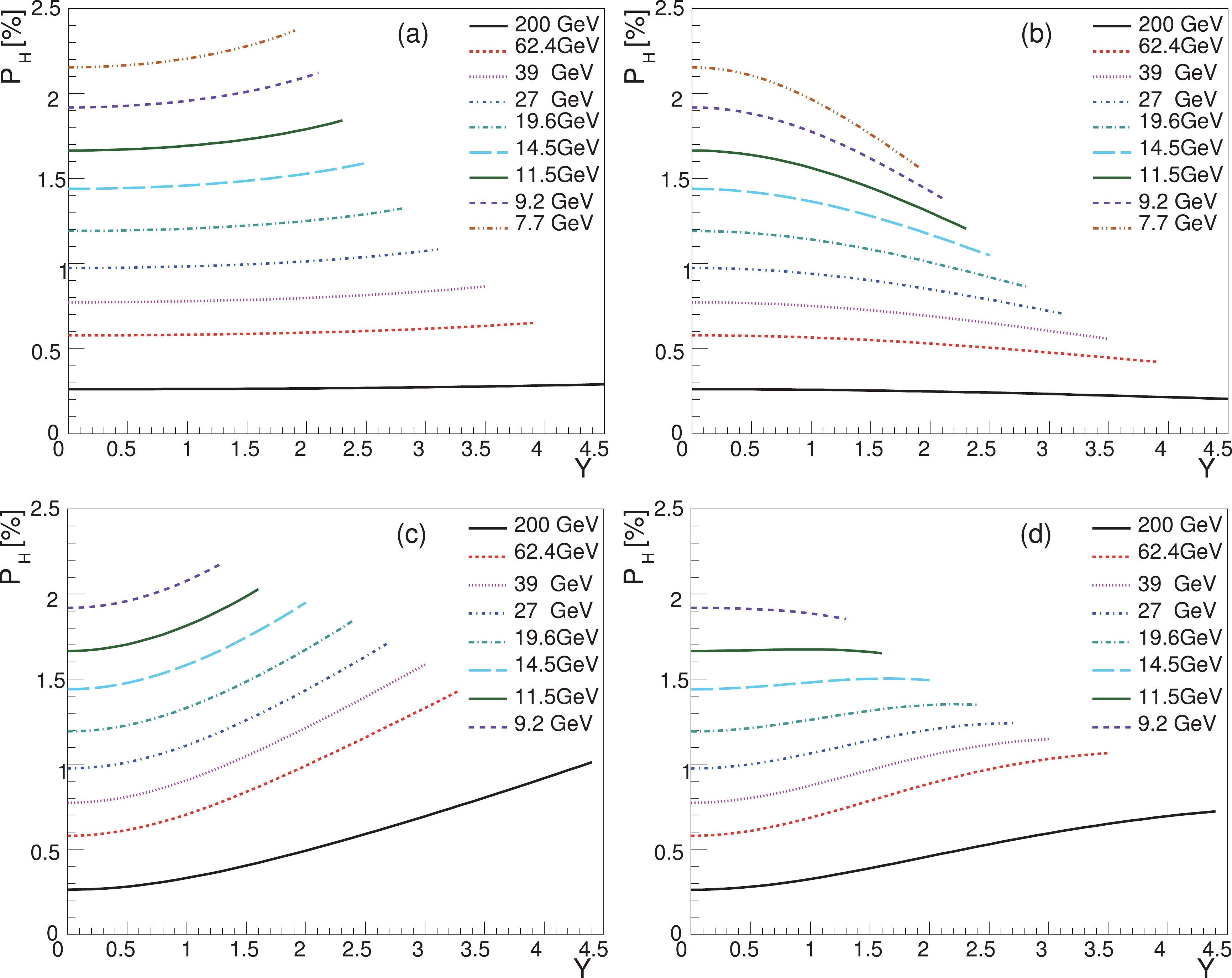
Figure 13. (color online) Global polarization of
$\Lambda$ (including$\overline{\Lambda}$ ) in the WS model as functions of rapidity in Au+Au collisions at different collision energies. We use the collision energy-dependent$\kappa_{0}$ , as determined in the right panel of Fig. 11. The impact parameter is set to$b = 1.2R_{A}$ , corresponding to a centrality of 20%-50%. The results in cases (a), (b), (c), and (d) are presented in panels (a), (b), (c), and (d) respectively.(b) Only
$ \kappa(Y) = \kappa_{0} $ is assumed to be constant in rapidity, while$ \left\langle p_{T}\right\rangle $ depends on the rapidity. The mid-rapidity values of$ \left\langle p_{T}\right\rangle $ are taken from the kaon data in Au+Au collisions in the collision energy range of 7.7-200 GeV [35, 36]. The rapidity dependence of$ \left\langle p_{T}\right\rangle $ is given by fitting the kaon data in Au+Au collisions at 62.4 GeV and 200 GeV [37, 38]. For the explicit form of$ \left\langle p_{T}\right\rangle $ as functions of rapidity and collision energy, see Appendix C. The result is shown in Fig. 13(b). We see that the polarization decreases with$ Y $ for each collision energy. At lower energies, the decreasing slope (the absolute value of the slope) is larger than that at higher energies. At 200 GeV, the polarization is almost a constant of rapidity.(c) A rapidity constant
$ \left\langle p_{T}\right\rangle $ is adopted, which takes its value at mid-rapidity at each energy, but the rapidity dependence of$ \kappa(Y) $ is assumed to take the form in Eq. (42). The result is shown in Fig. 13(c), where the polarization increases with rapidity. As the collision energy decreases, the slope increases. This increasing trend is stronger than that in cases (a) and (d) for the same collision energy.(d) Both
$ \kappa(Y) $ and$ \left\langle p_{T}\right\rangle $ depend on the rapidity. The rapidity dependence of$ \left\langle p_{T}\right\rangle $ is the same as that in case (b), while the rapidity dependence of$ \kappa(Y) $ is the same as that in case (c). The result is shown in Fig. 13(d). At high energies, the polarizations increase weakly with rapidity, while they are almost constants of rapidity at low energies. The result of this case is our main prediction.Note that the form of
$ \kappa(Y) $ in Eq. (42) used in cases (c) and (d) is valid for$ \mu_{B}\lesssim0.45 $ GeV; however, it is beyond such a$ \mu_{B} $ limit at 7.7 GeV. Therefore, the curves of 7.7 GeV in Figs. 13(c,d) are not shown because they are not reliable. -
We propose a geometric model for hadron polarization in heavy ion collisions, with an emphasis on the rapidity dependence. This model is based on the model of Brodsky, Gunion, and Kuhn as well as the Bjorken scaling model [25]. The starting point is the hadron rapidity distribution
$ {\rm d}^{3}N_{AA}/{\rm d}^{2}{{r}}_{T}{\rm d}Y $ as a function of the transverse position$ {{r}}_{T} $ in the overlapping region of colliding nuclei and the rapidity$ Y $ . We use the hard sphere and Woods-Saxon models for the nuclear density distribution, from which the thickness function is obtained. The rapidity distribution$ {\rm d}^{3}N_{AA}/{\rm d}x{\rm d}Y $ depending on the in-plane position$ x $ in the overlapping region can be derived from$ {\rm d}^{3}N_{AA}/{\rm d}^{2}{{r}}_{T}{\rm d}Y $ by integration over the out-plane position$ y $ . The average rapidity of hadrons can be obtained from the normalized distribution${\rm }{\rm d}^{3}N_{AA}/{\rm d}x{\rm d}Y $ or$ f(Y,x) $ . The collective logitudinal momentum$ \left\langle p_{z}\right\rangle $ is proportional to$ {\rm d}\ln f(Y,x)/{\rm d}Y $ . Then, the average local orbital angular momentum$ \left\langle L_{y}\right\rangle $ is proportional to the average shear of longitudinal momentum over$ x $ , which is a function of$ Y $ . The hadron polarization is assumed to be proportional to$ \alpha(Y)\left\langle L_{y}\right\rangle = \kappa(Y)\left\langle p_{T}\right\rangle \left\langle {\rm d}\ln f(Y,x)/{\rm d}Y{\rm d}x\right\rangle _{x,Y = 0} $ , where$ \alpha(Y) $ and$ \kappa(Y) $ are unknown rapidity functions characterizing transfer coefficients from the orbital angular momentum in the initial state to the hadron polarization in the final state. We make an ansatz for$ \kappa(Y) $ based on the similarity in hadron production between the case at forward rapidity and higher collision energy and that at central rapidity and lower collision energy. While the similarity is true for hadron production, it needs to be tested for hadron polarization by experiments. The parameter$ \kappa $ at mid-rapidity can be constrained by the polarization data of$ \Lambda $ and$ \overline{\Lambda} $ . The rapidity dependence of$ \left\langle p_{T}\right\rangle $ is obtained by fitting the data of kaons obtained by the BRAHMS and STAR collaborations. Finally, we make predictions for the rapidity dependence of the hadron polarization in the collision energy range of 7.7-200 GeV. These predictions can be tested by beam-energy-scan experiments at the Relativistic Heavy Ion Collider of Brookhaven National Lab. -
The authors thank C.M. Ko and J.Y. Jia for the insightful discussions.
-
In this appendix, we will derive the SLM
$ {\rm d}\ln f(Y,x)/ {\rm d}Y{\rm d}x $ in the HS model for the nuclear density distribution from Eqs. (17) and (18). The definitions of$ C_{1}^{\pm} $ and$ C_{2}^{\pm} $ are$\tag{A1} C_{1}^{\pm} = \int_{0}^{y_{m}}{\rm d}y\left[R_{A}^{2}-(x\mp b/2)^{2}-y^{2}\right]^{1/2}, $

$\tag{A2} C_{2}^{\pm} = \int_{0}^{y_{m}}{\rm d}y\left[R_{A}^{2}-(x\mp b/2)^{2}-y^{2}\right]^{-1/2}, $

where
$ y_{m} $ is the maximum of$ y $ at a fixed$ x $ $ y_{m} = \left[R_{A}^{2}-(|x|+b/2)^{2}\right]^{1/2}. \tag{A3}$

(A3) The analytical expressions of
$ C_{1}^{\pm} $ are$\tag{A4}\begin{aligned}[b] C_{1}^{+}\left(x\right) = \left\{\begin{split}& \frac{\pi}{4}\left[R_{A}^{2}-\left(x-\frac{b}{2}\right)^{2}\right], \quad\quad-(R_{A}-\frac{b}{2})<x\leqslant 0 \\ & \frac{1}{2}\sqrt{R_{A}^{2}-\left(x+\frac{b}{2}\right)^{2}}\sqrt{2bx}+ I_{-}(x), \quad\quad 0<x<R_{A}-\frac{b}{2} \end{split}\right. \end{aligned} $

$ \begin{array}{l} C_{1}^{-}\left(x\right) = \left\{\begin{split}& \frac{\pi}{4}\left[R_{A}^{2}-\left(x+\frac{b}{2}\right)^{2}\right], \quad\quad 0\leqslant x<R_{A}-\frac{b}{2}\\ & \frac{1}{2}\sqrt{R_{A}^{2}-\left(x-\frac{b}{2}\right)^{2}}\sqrt{-2bx}+I_{+}(x), \quad\quad -(R_{A}-\frac{b}{2})<x<0 \end{split} \right.\end{array}\tag{A5} $

(A5) where the function
$ I_{\pm}(x) $ is defined as$ I_{\pm}(x) = \frac{1}{2}\left[R_{A}^{2}-(x\pm b/2)^{2}\right]\arctan\frac{\sqrt{R_{A}^{2}-\left(x\mp b/2\right)^{2}}}{\sqrt{\mp2bx}}.\tag{A6}$

(A6) The analytical expressions of
$ C_{2}^{\pm} $ are$ C_{2}^{+}\left(x\right) =\left\{ \begin{split}& \arctan\frac{\sqrt{R_{A}^{2}-(x+b/2)^{2}}}{\sqrt{2bx}}, \quad 0<x<R_{A}-b/2\\ &\frac{\pi}{2}, \quad\quad -(R_{A}-b/2)<x\leqslant0 \end{split} \tag{A7} $

(A7) $ C_{2}^{-}\left(x\right) = \begin{cases} \dfrac{\pi}{2}, & 0\leqslant x<R_{A}-b/2\\ \arctan\dfrac{\sqrt{R_{A}^{2}-(x-b/2)^{2}}}{\sqrt{-2bx}}, & -(R_{A}-b/2)<x<0 \end{cases} \tag{A8} $

(A8) In terms of
$ C_{1}^{\pm} $ and$ C_{2}^{\pm} $ , we obtain the derivative of$ \ln f(Y,x) $ with respect to$ Y $ as$\begin{aligned}[b]\frac{{\rm d}\ln f(Y,x)}{{\rm d}Y} =& \frac{{\rm d}\ln({\rm d}N_{{pp}}/{\rm d}Y)}{{\rm d}Y}+\frac{1}{Y}\\&-\frac{1}{Y}\left[ 1+\frac{Y}{Y_{\rm L}}\cdot\frac{C_{1}^{+}-C_{1}^{-}}{C_{1}^{+}+C_{1}^{-}}\right] ^{-1},\end{aligned} \tag{A9}$

(A9) after which the derivative of
$ {\rm d}\ln f(Y,x)/{\rm d}Y $ with respect to$ x $ is$\tag{A10}\begin{aligned}[b] \frac{{\rm d}\ln f(Y,x)}{{\rm d}Y{\rm d}x} =& \frac{1}{Y_{L}}\left[1+\frac{Y}{Y_{\rm L}}\cdot\frac{C_{1}^{+}-C_{1}^{-}}{C_{1}^{+}+C_{1}^{-}}\right]^{-2}\left\{ -\frac{x(C_{2}^{+}-C_{2}^{-})-(b/2)(C_{2}^{+}+C_{2}^{-})}{(C_{1}^{+}+C_{1}^{-})}\right. +\frac{(C_{1}^{+}-C_{1}^{-})\left[x(C_{2}^{+}+C_{2}^{-})-(b/2)(C_{2}^{+}-C_{2}^{-})\right]}{(C_{1}^{+}+C_{1}^{-})^{2}} \\ &-2\sqrt{2b|x|}(|x|+b/2) \sqrt{R_{A}^{2}-(|x|+b/2)^{2}} \left.\frac{C_{1}^{+}\theta(-x)+C_{1}^{-}\theta(x)}{(C_{1}^{+}+C_{1}^{-})^{2}}\right\} , \end{aligned} $

(A10) where we have used
$ \frac{{\rm d}}{{\rm d}x}\int_{0}^{a(x)}{\rm d}yb(x,y) = \int_{0}^{a(x)}{\rm d}y\frac{\partial b(x,y)}{\partial x}+b(x,a(x))\frac{{\rm d}a(x)}{{\rm d}x}. \tag{A11}$

(A11) -
There is a similarity in hadron production between the case at forward rapidity and higher collision energy and that at central rapidity and lower collision energy. Thus, the baryon number density or baryon chemical potential is the relevant physical quantity in both cases. Therefore, if we neglect the system size effect, we can make an ansatz for
$ \kappa(Y) $ based on this correspondence.By fitting the data in Fig. 8(b), we find the following energy behavior for
$ \kappa_{0}\equiv\kappa(Y = 0) $ ,$ \kappa_{0} = \frac{2.8}{\left(0.05+\sqrt{s_{NN}}/200\right)^{0.6}}. \tag{B1}$

(B1) The collision energy dependence of the baryon chemical potential at mid-rapidity can be given by [39]
$ \mu_{B}(0)\equiv\mu_{B}(Y = 0) = \frac{1.3075}{1+0.288\sqrt{s_{NN}}}\: \rm{GeV}. \tag{B2}$

(B2) We can solve
$ \sqrt{s_{NN}} $ as a function of$ \mu_{B}^{(0)} $ and obtain$ \kappa_{0} = \frac{2.8}{\left[0.05+\left(1.3075/\mu_{B}(0)-1\right)/57.6\right]^{0.6}}, \tag{B3}$

(B3) in the range of
$ \mu_{B}^{(0)}\lesssim0.45 $ GeV, i.e., in the collision energy range of 7.7-200 GeV. We can generalize the above expression to other rapidity values as$ \kappa(Y) = \frac{2.8}{\left[0.05+\left(1.3075/\mu_{B}(Y)-1\right)/57.6\right]^{0.6}}, \tag{B4}$

(B4) by taking the following parameterization of
$ \mu_{B}(Y) $ [40]$ \mu_{B}(Y) = \mu_{B}(0)+\left(0.09527-0.01594\log\sqrt{s_{NN}}\right)Y^{2}. \tag{B5}$

(B5) -
The average transverse momentum
$ \left\langle p_{T}\right\rangle $ also has rapidity dependence. The$ \left\langle p_{T}\right\rangle $ data for kaons at different rapidities are measured by the BRAHMS collaboration at 200 and 62 GeV [37, 38], which can be parameterized as$ \left\langle p_{T}\right\rangle _{Y}\approx\left\langle p_{T}\right\rangle _{0}\exp\left(-\frac{Y^{2}}{2Y_{\rm L}^{2}}\right), \tag{C1}$

(C1) where
$ \left\langle p_{T}\right\rangle _{0}\equiv\left\langle p_{T}\right\rangle _{Y = 0} $ denotes the average transverse momentum at mid-rapidity; see Fig. C1. Here,$ \left\langle p_{T}\right\rangle _{0} $ also depends on the collision energy and can be parameterized as
Figure C1. (color online) Average transverse momentum
$\left\langle p_{T}\right\rangle$ for kaons as functions of rapidity in central Au+Au collisions.$ \left\langle p_{T}\right\rangle _{0} = 0.41634+0.030644s_{NN}^{1/4}-0.0011547s_{NN}^{1/2}, \tag{C2}$

(C2) following STAR data for kaons at
$ \sqrt{s_{NN}} = $ 7.7-200 GeV [35, 36], where the unit of$ \left\langle p_{T}\right\rangle _{0} $ is GeV and$ s_{NN}^{1/2} $ takes the dimensionless value of the collision energy in GeV; see Fig. C2.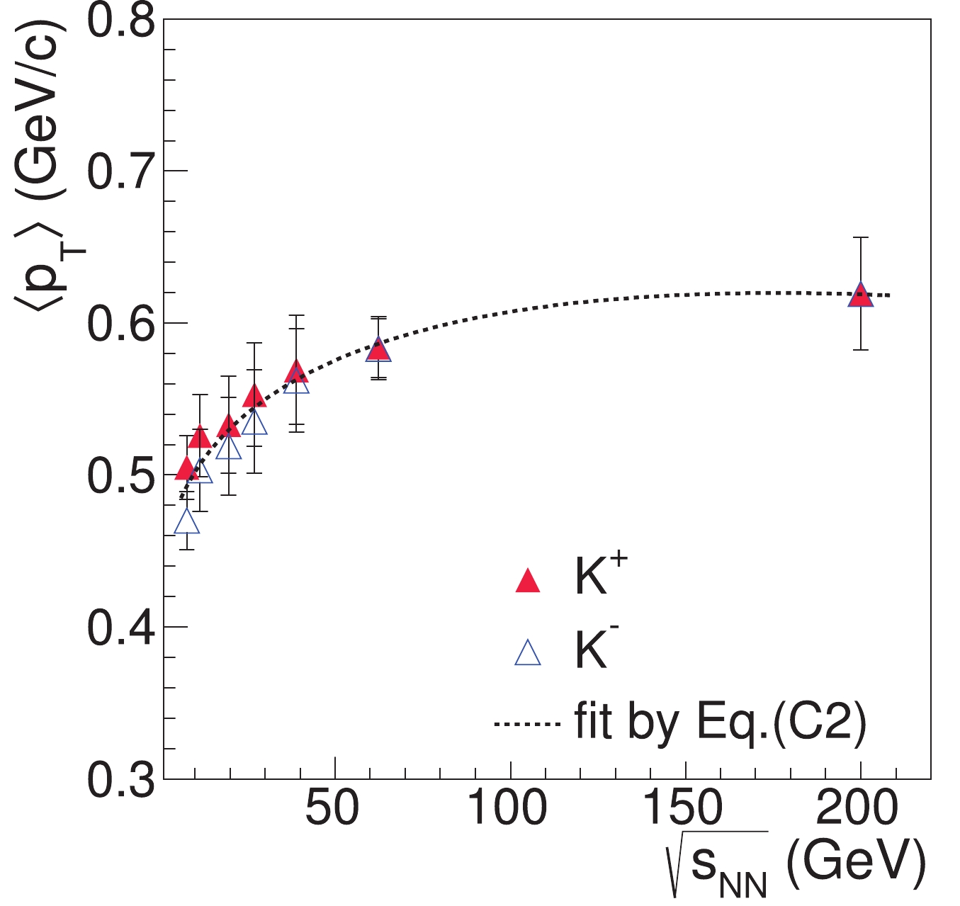
Figure C2. (color online) Average transverse momentum at mid-rapidity
$\left\langle p_{T}\right\rangle _{0}$ for kaons as functions of collision energies in semi-central (40%-50%) Au+Au collisions.
Rapidity dependence of global polarization in heavy ion collisions
- Received Date: 2020-06-16
- Available Online: 2021-01-15
Abstract: We use a geometric model for hadron polarization in heavy ion collisions with an emphasis on the rapidity dependence. The model is based on the model of Brodsky, Gunion, and Kuhn, as well as the Bjorken scaling model. We make predictions regarding the rapidity dependence of global


 DownLoad: