


 Abstract
 HTML
HTML Reference
 Related
 PDF
PDF


-
The accelerated expansion of the universe has been discovered by analyzing distant and nearby supernovae in 1998 [1,2]. This discovery indicated the return of the cosmological constant proposed by Einstein, termed dark energy. Data from the last two decades indicate that the cosmological constant is a very tiny positive value on the order of
$ 10^{-124} $ in Planck units [1-14]. In Einstein's theory of general relativity, the cosmological constant coincides with the vacuum energy [15]. The vacuum energy contains the contribution of vacuum fluctuations described by quantum mechanics. However, the theoretical expectations for the vacuum energy exceed the observed value by 124 orders of magnitude [16]. This gives rise to the cosmological constant fine tuning problem [17]. Theorists have proposed numerous theoretical models [18-24] to solve this problem. However, these theories can only partially solve this problem or avoid the vacuum energy caused by quantum fluctuations. It is still one of the central problems in theoretical physics and cosmology.We have investigated some high-dimensional theories [25-46] to solve this problem. Among these theories, the Randall-Sundrum (RS) two-brane model [28] has attracted our attention. In this model, the hierarchy problem of why there is such a large discrepancy between the electroweak scale/Higgs mass
$ M_{EW}\sim1{\rm{TeV}} $ and the Planck mass$ M_{pl}\sim10^{16}\;{\rm{TeV}} $ is solved very well. The warp factor${\rm e}^{-2kr\pi}$ originating from the background metric generates a large hierarchy, but requires only$ kr\approx10 $ . This large hierarchy problem is somewhat similar to the cosmological constant fine tuning problem. However, the RS model has a negative brane tension, which results in the instability of the visible brane. Furthermore, a zero cosmological constant on the visible 3-brane is not consistent with presently observed data [29,47]. Therefore, one solution of the fine tuning problem is to find a new mechanism in the RS model that renders the effective cosmological constant a very small positive value, which is compatible with present cosmological observations.In this paper, we show that this problem can be solved using the
$ (n+1) $ -dimensional (-d) generalized RS braneworld model [29] with two$ (n-1) $ -branes (the visible and hidden branes) instead of two 3-branes. In this model, the induced cosmological constant$ \Omega $ on the visible brane appears naturally. For the negative induced cosmological constant, there is a solution with positive visible and hidden brane tension [48-52]. For$ -\Omega $ on the order of$ 10^{-124} $ , we obtain the solutions corresponding to the magnitude of the warp factor.To remain consistent with observations, the negative induced cosmological constant must be transformed into a positive effective cosmological constant. We investigate the case where the scale factors on the visible brane evolve with different rates by adopting an anisotropic metric ansatz [53]. The Hubble parameters are obtained by solving the Einstein field equation. We obtain a positive effective cosmological constant
$\Omega_{\rm eff}$ consistent with observations on the order of$ -\Omega $ . This result suggests that cosmic acceleration is intrinsically an extra-dimensional phenomenon. The Hubble parameter$ H_{1}(z) $ as a function of redshift$ z $ is consistent with most of the cosmic chronometers dataset. -
We start with an
$ (n+1) $ -d generalized RS braneworld model. The total action$ S_{n+1} $ is composed of the bulk action and two$ (n-1) $ -brane actions:$ S_{\rm bulk} = \int {\rm d}^{n}x{\rm d}y\sqrt{-G}(M^{n-1}_{n+1}R-\Lambda) , $

(1) $ S_{\rm vis} = \int {\rm d}^{n}x\sqrt{-g_{\rm vis}}({\cal{L}}_{\rm vis}-V_{\rm vis}), $

(2) $ S_{\rm hid} = \int {\rm d}^{n}x\sqrt{-g_{\rm hid}}({\cal{L}}_{\rm hid}-V_{\rm hid}), $

(3) where
$ \Lambda $ is a bulk cosmological constant of order$ 1 $ in Planck units (the vacuum energy described by quantum mechanics),$ M_{n+1} $ denotes an$ (n+1) $ -d fundamental mass scale,$ G_{AB} $ is the$ (n+1) $ -d metric tensor,$ R $ is the$ (n+1) $ -d Ricci scalar,$ {\cal{L}}_{i} $ and$ V_{i} $ are the matter field Lagrangian and the tension of the$ i $ -th brane, respectively, and$i = {\rm hid}$ or${\rm vis}$ . The total action$ S_{n+1} $ is stationary with respect to arbitrary variations in$ G_{AB} $ if and only if$ \begin{split} R_{AB}-\frac{1}{2}G_{AB}R =& \frac{1}{2M^{n-1}_{n+1}}\bigg\{-G_{AB}\Lambda+\sum\limits_{i}[T^{i}_{AB}\delta(y-y_{i})\\ &-G_{ab}\delta_{A}^{a}\delta_{B}^{b}V_{i}\delta(y-y_{i})]\bigg\}, \end{split} $

(4) where capital Latin
$ A,B $ indices run over all spacetime coordinate labels$ 0, 1, 2, \cdots, n $ , lowercase Latin$ a,b = 0,1,2,\cdots,n-1 $ ,$ R_{AB} $ and$ T^{i}_{AB} $ are the$ (n+1) $ -d Ricci and the energy-momentum tensors, respectively, and$ y_{i} $ represents the position of the$ i $ -th brane in the$ (n+1) $ -th coordinate. The$ (n+1) $ -d energy-momentum tensor of an anisotropic perfect fluid is$T^{iA}_{B} = {\rm diag}[-\rho_{i},p_{i1},p_{i2},\cdots, p_{i(n-1)},0]$ . In this generalized RS model, the metric ansatz satisfying the Einstein field equations, Eq. (4), is of the form:$ {\rm d}s^{2} = G_{AB}{\rm d}x^{A}{\rm d}x^{B} = {\rm e}^{-2A(y)}g_{ab}{\rm d}x^{a}{\rm d}x^{b}+r^{2}{\rm d}y^{2}, $

(5) where
$ g_{ab} $ is the$ n $ -d metric tensor,${\rm e}^{-2A(y)}$ is known as the warp factor, and$ y $ is the extra-dimensional coordinate of length$ r $ . Combining Eq. (4) with Eq. (5), each energy-momentum tensor is given by$T^{ia}_{b} = {\rm diag}[-c_{i},c_{i},\cdots,c_{i}]$ . This is similar to the RS model, in which each 3-brane Lagrangian separates out a constant vacuum energy [28]. Then, the equations of$ A'' $ and$ A'^{2} $ are given by$ A'' = \frac{2\Omega {\rm e}^{2A}}{(n-1)(n-2)}+\frac{\sum_{i}\delta(y-y_{i}){\cal{V}}_{i}}{2M^{n-1}_{n+1}(n-1)}, $

(6) $ A'^{2} = \frac{2\Omega {\rm e}^{2A}}{(n-1)(n-2)}+k^{2}, $

(7) where we redefine the brane tension
$ {\cal{V}}_{i}\equiv V_{i}-c_{i} $ , the constant$ k\equiv\sqrt{-\Lambda/[M^{n-1}_{n+1}n(n-1)]}\simeq $ the Planck mass, and the arbitrary constant$ \Omega $ corresponds to the induced cosmological constant on the visible brane. Meanwhile, the$ n $ -d Einstein field equations with this induced cosmological constant are given by$ \widetilde{R}_{ab}-\frac{1}{2}g_{ab}\widetilde{R} = -\Omega g_{ab}, $

(8) where
$ \widetilde{R}_{ab} $ and$ \widetilde{R} $ are the$ n $ -d Ricci tensor and Ricci scalar, respectively. The arbitrary constant$ \Omega $ corresponds to the induced cosmological constant on the visible brane. In this paper, we only consider the situation where$ \Omega<0 $ because$ \Omega>0 $ always brings about a negative tension on the visible brane, which results in instability.For
$ \Omega<0 $ , the warp factor satisfying Eqs. (4) and (5) is obtained:$ A = -\ln[\omega\cosh(k|y|+c_{-})], $

(9) where
$ \omega^{2}\!\equiv\!-2\Omega/[(n-1)(n-2)k^{2}] $ and$ c_{-} = \ln[(1-\sqrt{1-\omega^{2}})/\omega] $ for considering the normalization at the extra-dimensional fixed coordinate$ y = 0 $ . Setting${\rm e}^{-A(r\pi)}\equiv10^{-m}$ ,$ x\equiv\pi kr $ , and$ \omega^{2}\equiv10^{-l} $ [29,54], we obtain the following from Eq. (9):$ {\rm e}^{-x} = \frac{10^{-m}}{2}\bigg[1\pm\sqrt{1-10^{-(l-2m)}}\;\bigg], $

(10) where the induced cosmological constant has an upper bound (
$l_{\min} = 2m$ ) to ensure that the value in the square root is greater than zero. Eq. (10) has two solutions that give rise to the required warping. For$ (l-2m)\gg1 $ , the first solution corresponds to the visible brane tension$ {\cal{V}}_{\rm vis} = -4(n-1)M^{n-1}_{n+1}k. $

(11) Here, the visible brane is unstable because the visible brane tension is negative. We do not consider this solution in the following. The second solution is
$ x = (l-m) \ln10+\ln4 $ , which is consistent with Eq. (21) in Ref. [29]. Both the visible and the hidden brane are stable because both brane tensions are$ {\cal{V}}_{\rm vis} = {\cal{V}}_{\rm hid} = 4(n-1)M^{n-1}_{n+1}k>0. $

(12) -
The
$ n $ -d effective theory can be obtained by substituting Eq. (5) into the bulk action Eq. (1). We can obtain the scale of gravitational interactions from the curvature term:$ S_{\rm eff}\supset\int {\rm d}^{n}x\int_{-\pi}^{\pi}{\rm d}y\sqrt{-g}M^{n-1}_{n+1}r{\rm e}^{-(n-2)A(kry)}\tilde{R}. $

(13) Substituting Eq. (9) into Eq. (13) and performing the integral of
$ y $ , we can obtain an$ n $ -d effective action. We find that$ M_{n} $ depends only weakly on$ r $ in the large$ kr $ limit when$\omega^{2}\ll {\rm e}^{-kr\pi}$ . Thus,$ M_{n} $ is given by$ M^{n-2}_{n}\simeq\frac{2M^{n-1}_{n+1}}{(n-2)k}[1-{\rm e}^{-(n-2)kr\pi}]. $

(14) The hierarchy problem cannot be solved in this
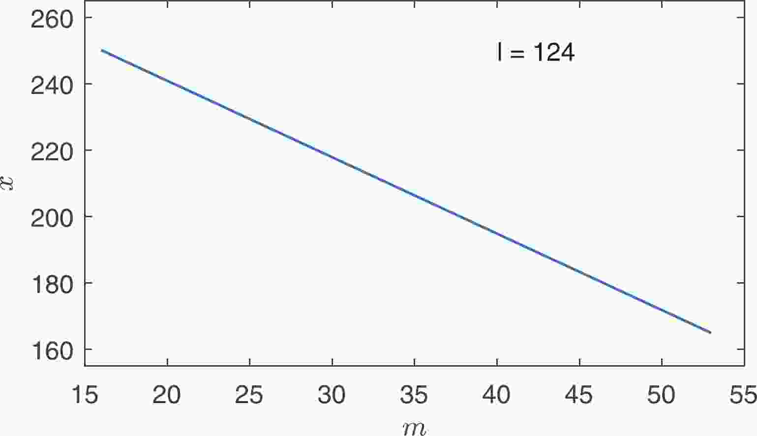
$ (n+1) $ -d generalized RS braneworld model because we can not determine the physical mass by means of renormalization.In Fig. 1, if
$ l\sim124 $ , i.e., the magnitude of the induced cosmological constant is on the order of$ -124 $ in Planck units, we get the second solution$ x\simeq160-250 $ , which corresponds to$ m\simeq53-16 $ when$ m $ satisfies the condition$ l-2m\gg1 $ . Different warp factors correspond to different solutions to ensure$ l\sim124 $ . The cosmological constant fine tuning problem can be partially solved in this mechanism only by requiring$ kr\simeq50-80 $ .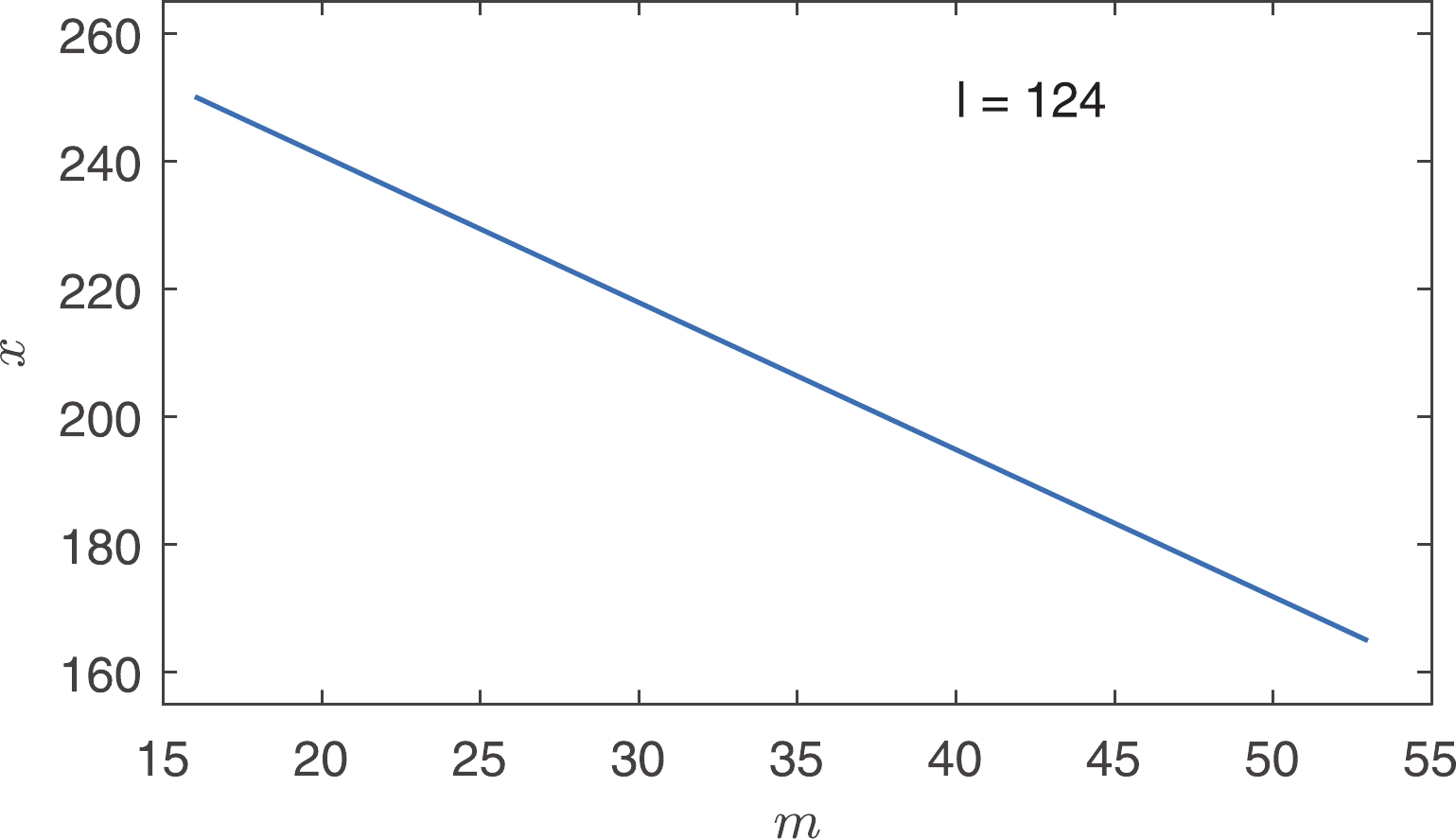
Figure 1. (color online) Graph of
$x( = kr\pi)$ versus$m = 16-53$ for$l = 124$ and negative brane cosmological constant.The remaining unsolved problem is how to transform a negative cosmological constant into a positive one. If we choose an isotropic metric, one can obtain
$ H^{2} = \Omega $ . Here, because$ \Omega<0 $ , there is no real solution, which is not consistent with presently observed data. Therefore, we choose an anisotropic metric ansatz of the form [53]$ g_{ab} = {\rm diag}[-1,a_{1}^{2}(t),a_{2}^{2}(t),a_{3}^{2}(t),\cdots,a_{n-1}^{2}(t)], $

(15) where
$ a_{i} $ is the scale factor. In this paper, we investigate the simplest case, in which the scale factors on the visible brane evolve only with two different rates. With the negative induced cosmological constant$ \Omega\sim-10^{-124} $ , we obtain the solutions of Eq. (8):$ H_{1} = -\frac{\eta_{1}}{n-1}\tan\alpha+\eta_{2}\sec\alpha , $

(16) $ H_{2} = -\frac{\eta_{1}}{n-1}\tan\alpha-\eta_{3}\sec\alpha , $

(17) where the Hubble parameter
$ H\equiv\dot{a}/a $ ,$ \alpha = \eta_{1}t+\theta_{0} $ , and$ \theta_{0} $ is the initial phase angle, which is determined by the scale of the formation of the brane. In other words, the value of$ \theta_{0} $ must ensure that the presently observed three-dimensional (3D) scale can be found. The terms$ \eta_{1} $ ,$ \eta_{2} $ , and$ \eta_{3} $ are respectively$ \eta_{1} = \sqrt{\frac{-2(n-1)\Omega}{n-2}}, \eta_{2} = \sqrt{\frac{-2\Omega n_{2}}{(n-1)n_{1}}}, \eta_{3} = \sqrt{\frac{-2\Omega n_{1}}{(n-1)n_{2}}}, $

where
$ n_{1} $ and$ n_{2} $ are the number of dimensions, which evolve with two different rates. We choose$ n_{1} = 3 $ , which is most in line with the presently observed 3D space universe. From the time of formation of the brane$ t\equiv0 $ to the present time ($ t\sim10^{61} $ in Planck units), it is easy to satisfy the condition in which the 3D scale factor is expanding all the time because$ \eta_{1} $ is a very tiny value, on the order of$ \sqrt{-\Omega}\simeq10^{-62} $ in Planck units.In Fig. 2,
$ H_{1} $ and$ H_{2} $ are shown as functions of$ \alpha $ . The three curves in the upper half of Fig. 2 correspond to$ H_{1} $ at$ n_{2} = 1, 3, 5 $ , respectively. It is clear that$ H_{1} $ has a lower bound as long as$ n_{2}\neq1 $ :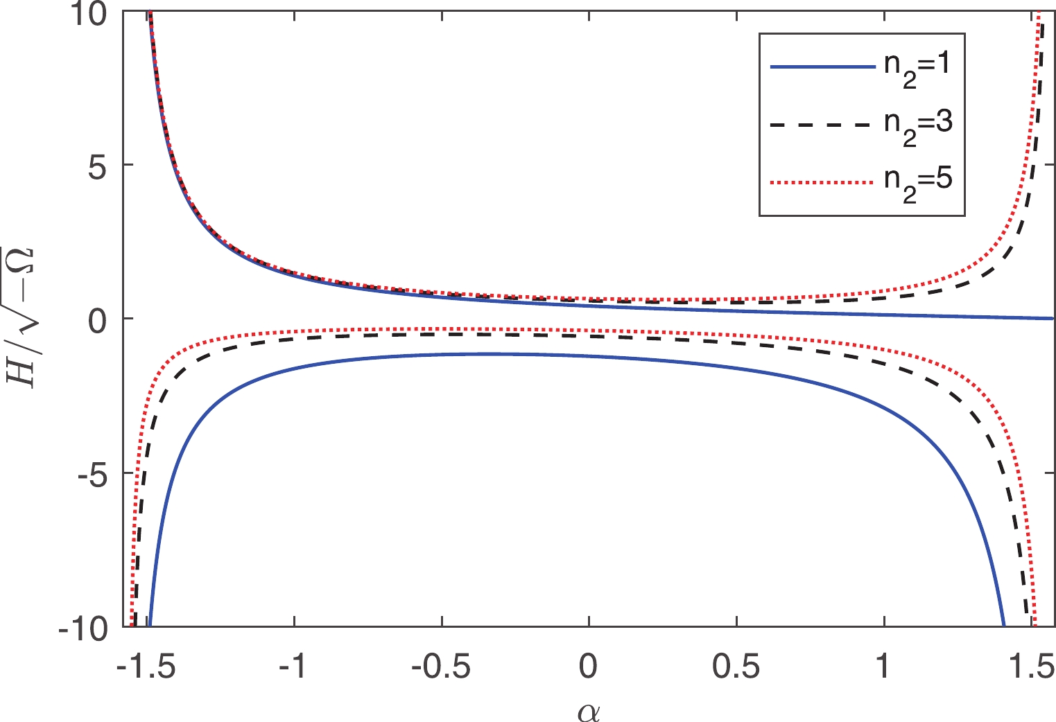
Figure 2. (color online) Hubble parameters
$H_{1}$ (> 0) and$H_{2}$ (< 0) with$n_{1} = 3$ . Three different extra dimensions$n_{2} = 1, 3, 5$ correspond to the solid (blue) curve, the dashed (black) curve, and the dotted curve (red) respectively.$ H_{1\min} = \sqrt{\eta_{2}^{2}-\eta_{1}^{2}/(n-1)^{2}}, $

(18) where
$\alpha_{\min} = \arcsin\{\sqrt{n_{1}/[n_{2}(n_{1}+n_{2}-1)]}\}$ . Here, we see that the number of extra dimensions on the brane cannot be one; otherwise, the time-independent positive effective cosmological constant cannot be obtained [54]. In the limit$ n_{2}\rightarrow\infty $ , the lower bound of the Hubble parameter is$H_{1\min}\simeq\sqrt{-6\Omega}/3$ . In the region near$\alpha_{\min}$ ,$ H_{1} $ is close to a constant on the order of$ \sqrt{-\Omega} $ . Comparing with the 3D Friedmann equation with$ K = 0 $ , the effective cosmological constant is on the order of$ -\Omega $ because in the region near$\alpha_{\min}$ we have$ H_{1}^{2}\sim-\Omega\equiv\Omega_{\rm eff}>0. $

(19) This is an important result. It tells us that the negative induced cosmological constant
$ \Omega $ can be transformed into a positive effective cosmological constant$\Omega_{\rm eff}$ because of the evolution of the extra dimensions. Cosmic acceleration is intrinsically an extra-dimensional phenomenon, and the cosmological constant fine tuning problem can be solved using this extra-dimensional evolution.From Eqs. (16) and (17), we can obtain the scale factors
$ a_{1} $ and$ a_{2} $ . Furthermore, we obtain the volume of the visible brane$ V_{b} = a_{1}^{n_{1}}a_{2}^{n_{2}} = a_{10}^{n_{1}}a_{20}^{n_{2}}, $

(20) where
$ a_{10} $ and$ a_{20} $ are the scale factors when the brane forms. We choose$ a_{10} = a_{20} $ because there is no reason to make them different when the brane has not evolved yet. If the scale of the brane just formed is on the order of$ 10^{35} $ in Planck units ($ \sim1m $ ), to form the presently observed 3D scale on the order of$ 10^{61} $ , the scale of extra dimensions must be on the order of$ 10^{9} $ with$ n_{2} = 3 $ . Therefore, the scale of extra dimensions can be much larger than the Planck length, which leads to the fact that physics are still valid in this model. The three curves in the lower half of Fig. 2 show$ H_{2} $ with$ n_{2} = 1, 3, 5 $ , respectively. With an increase in$ n_{2} $ , the scale of the brane just formed decreases; meanwhile, this result ensures that the extra dimensions will not reduce to the Planck length at the present time.$ \theta_{0} $ is close to$ -\pi/2 $ as long as$ a_{10} $ is tiny. Therefore, in the region of$ \theta_{0}+\pi/2\ll\eta_{1}t\ll\pi/2 $ , we obtain$ H_{1}\simeq\frac{1}{n_{1}+n_{2}}\bigg[1+\sqrt{\frac{(n_{1}+n_{2}-1)n_{2}}{n_{1}}}\;\bigg]\frac{1}{t}. $

(21) At
$ n_{2} = 1 $ ,$ H_{1} $ is approximately$ 1/2t $ , which is similar to the radiation-dominant eras. In the limit$ n_{2}\rightarrow\infty $ ,$ H_{1}\simeq\sqrt{3}/3t $ .The blue solid curve in Fig. 3 shows
$ H_{1}(z) $ as a function of redshift$ z $ with$ n_{2} = 5 $ . To best fit the cosmic chronometers dataset, we obtain the present time$ t = t_{0} $ when$\alpha_{0} = \alpha_{\min}+0.25$ . Therefore,$ H_{1}(z) $ has a minimum at$ z\sim0.1 $ . Between$ z = 0 $ and$ z\sim0.1 $ ,$ H_{1}(z) $ is slowly decreasing, which is similar to most of the cosmic chronometers dataset. When$ z>0.1 $ ,$ H_{1}(z) $ is monotonically increasing, which is in agreement with the cosmic chronometers dataset, except at$ z = 1.965 $ . The Hubble parameter is slightly larger than that in the cosmic chronometers dataset at this redshift. The deceleration parameter$ q $ is given by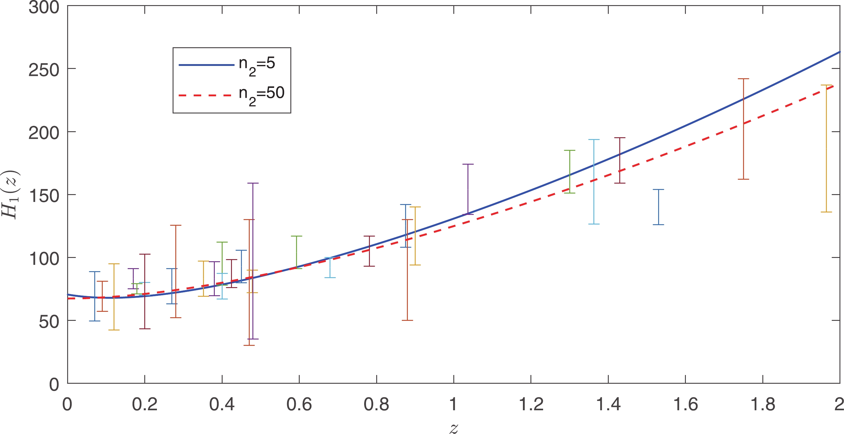
$ q\equiv-\ddot{a}_{1}a_{1}/\dot{a}_{1}^{2} = -1-\frac{\dot{H}_{1}}{H_{1}^{2}}, $

(22) where
$ \dot{H}_{1} = -\frac{\eta_{1}^{2}}{n-1}\sec^{2}\alpha+\eta_{1}\eta_{2}\sec\alpha\tan\alpha. $

(23) From Eq. (22), we obtain the time
$ t_{q = 0} $ from deceleration to accelerated expansion (namely, deceleration parameter$ q = 0 $ ). Using Eq. (16), the 3D scale factor is given by$ a_{1} = c_{0}(\cos\alpha)^{\textstyle\frac{1}{n-1}}(\sec\alpha+\tan\alpha)^{\textstyle\frac{1}{n-1}\sqrt{\frac{n_{2}(n-2)}{n_{1}}}}, $

(24) where
$ c_{0} $ is the integral constant. Combining the definition of redshift$ z = a_{0}/a-1 $ and the present time$ t_{0} $ , we obtain$ z\approx0.35 $ at$ t = t_{q = 0} $ . The red dashed curve in Fig. 3 shows that$ H_{1}(z) $ is a monotonic curve when$ n_{2} = 50 $ . We obtain the present time$ t = t_{0} $ when$\alpha = \alpha_{\rm min}$ . This curve is in good agreement with the cosmic chronometers dataset. With an increase in$ n_{2} $ , the slope of$ H_{1}(z) $ becomes smaller, so that it is more consistent with the cosmic chronometers dataset at$ z = 1.965 $ . The evolution of the 3D space shifts from deceleration to acceleration when the redshift$ z\approx0.44 $ . -
In conclusion, we investigate an
$ (n+1) $ -d generalized Randall-Sundrum model with a bulk cosmological constant of order$ 1 $ in Planck units (the vacuum energy caused by quantum fluctuations). The induced cosmological constant$ \Omega $ on the visible brane appears naturally in this model. Both the visible and hidden branes are stable because their tensions are positive when$ \Omega<0 $ . Adopting an anisotropic metric ansatz, we obtain the positive effective cosmological constant$\Omega_{\rm eff}$ on the order of$ -\Omega\sim10^{-124} $ and only require a solution$ \simeq50-80 $ . Therefore, the cosmological constant fine tuning problem can be solved quite well.Meanwhile, the Hubble parameter
$ H_{1}(z) $ as a function of redshift is consistent with most of the cosmic chronometers dataset. The evolution of the 3D space naturally shifts from deceleration to acceleration when the redshift$ z\approx0.4 $ . It is worth noting that we did not introduce the matter and radiation energy-momentum tensor in a perfect fluid form when we obtained the above results. This result suggests that the evolution of the 3D scale factor (cosmic acceleration period or the like-matter-dominated period) is intrinsically an extra-dimensional phenomenon. This can be seen as a dynamic model of dark energy that is driven by the evolution of the extra dimensions on the brane.
Fine tuning problem of the cosmological constant in a generalized Randall-Sundrum model
- Received Date: 2020-05-13
- Accepted Date: 2020-07-13
- Available Online: 2020-12-01
Abstract: To solve the cosmological constant fine tuning problem, we investigate an


 DownLoad: