


 Abstract
 HTML
HTML Reference
 Related
 PDF
PDF


-
The problem of calculating the moment of inertia (
$ {\rm MOI} $ ) of even-even nuclei has received considerable attention since the 1950s [1-3]. The hydrodynamical model, first introduced by Bohr [4], considered the nucleus as a droplet of incompressible irrotational fluid. As a consequence, the collective motion of the nucleus was pictured as a quadrupole of classical oscillations similar to those of the liquid droplet discussed in detail by Rayleigh [5]. This description of Bohr led to a simple relationship between the moment of inertia$ \Im $ and the deformation parameter$ \beta $ ,$ \Im = 3B\beta^2 $ , where$ B $ is the inertial parameter. This relationship is referred to as Bohr's formula. In the particular case of small oscillations and, hence,$ R(\theta,\phi) $ , the radial coordinate of the surface at the polar coordinates$ (\theta,\phi) $ can be approximated as$ R_0 $ , i.e., the radius of the spherical shape of the liquid drop at equilibrium. Rayleigh's calculations indicated that$ B = \dfrac{\rho R_{0}^{5}}{2} $ . The values of the$ {\rm MOI} $ calculated using Bohr's formula with the values of$ B $ derived by Rayleigh are five times smaller than those obtained experimentally. Furthermore, one cannot explain the$ {\rm MOI} $ of deformed nuclei by considering the extreme case of a rigid deformed shape [6].An alternative approach used to describe the
$ {\rm MOI} $ of deformed nuclei was based on the cranking model introduced by Inglis [7]. In this model, the kinetic energy of rotation is obtained by considering the motion of the nucleons in the rotating self-consistent field. In contrast to the hydrodynamical model, the resultant values for the cranking model are found to be 2-3 times larger than those for the experimental ones. Therefore, both models-Bohr's hydrodynamical model and Inglis's cranking model-have been modified by several authors [2, 8-14]. Recently, a valuable thorough quantitative comparison of predictions for both form factor and moment of inertia obtained using four different models (Hartree-Fock, cranking model, rigid rotator, and irrotational fluid flow) for the rare earth nuclei$ ^{154}{\rm Sm} $ ,$ ^{156}{\rm Gd} $ ,$ ^{164}{\rm Dy} $ ,$ ^{166,168}{\rm Er} $ , and$ ^{174}{\rm Yb} $ was proposed in [9]. The authors of [9] extended their work to observe the electromagnetic form factors for some${\rm Hf}$ isotopes of odd masses [15].In this study, we assumed that Rayleigh's approach within the approximation of
$ R $ to$ R_0 $ is the reason for the poor agreement of Bohr's results. Accordingly, we expanded$ R $ about$ R_0 $ and worked out the second and third terms of this expansion in addition to the first one, which has already been discussed by Rayleigh. The obtained equation, which is referred to as the modified form of Bohr's relationship, is verified on axially symmetric nuclei of atomic mass ranging between 150 and 190 as well as on a number of triaxially symmetric nuclei. The results of both the modified and original formulas of Bohr are compared with the experimental data presented in Table 1 as well as with the numerical values proposed in [9], as presented in Table 2. It is found that, even though the agreement with experimental data as well as with numerical ones is not so good, the enhancements in the results are remarkable-the ratios of the modified Bohr results (current work) to the experimental results are approximately 0.6 to sometimes 0.7 instead of 0.2 in the case of Bohr's original work. -
The surface of the nucleus that is represented in polar coordinates by
$ R(\theta,\phi) $ can be expanded in spherical harmonics as follows [1]$ R(\theta,\phi) = R_0\left(1+\sum\limits_{\mu}\alpha_{\lambda\mu}^{*}Y_{\lambda\mu}(\theta,\phi)\right), $

(1) where
$ R_{0} $ is the radius of the spherical nucleus (i.e., when all$ \alpha_{\lambda\mu} $ have vanished). Because of the reality of$ R $ ,$\displaystyle \alpha_{\lambda\mu}^{*} = (-1)^{\mu}\alpha_{\lambda,-\mu} $ , and because$ R $ is rotationally invariant,$ \displaystyle \alpha_{\lambda\mu} = \sum_{\nu}D_{\mu\nu}^{\lambda}(\theta_{j})a_{\lambda\nu} $ , where$ D_{\mu\nu}^{\lambda}(\theta_{j}) $ is the transformation operator,$ \alpha_{\lambda\mu} $ and$ a_{\lambda\nu} $ are the deformation parameters in space-fixed [16] and body-fixed coordinates, respectively, and$ \theta_{j} $ are the Euler angles connecting the space-fixed and rotated frames (where$ j = 1,2,3 $ ) [17,18]. The functions$ Y_{\lambda\mu} $ are spherical harmonics of the order$ \lambda,\mu $ .If we consider only the quadratic deformation of order 2 (i.e.,
$ \lambda = 2 $ ) and choose the rotating coordinates to coincide with the principal coordinates, then one can easily verify that$ a_{21} = a_{2,-1} = 0 $ ,$ a_{22} = a_{2,-2}\neq 0 $ , and$ a_{20}\neq 0 $ (we will drop the index$ \lambda = 2 $ from the deformation parameters henceforth). Therefore, we are now left with only two parameters$ a_{0} $ and$ a_{2} $ to describe the shape of the nucleus and three Euler angles to specify the orientation of the principal axes of the nucleus. Sometimes, it is more convenient to use$ \beta $ and$ \gamma $ instead of$ a_0 $ and$ a_2 $ with the definition$ a_{0} = \beta\cdot\cos(\gamma) $ and$a_{2} = \dfrac{\beta}{\sqrt{2}}\cdot \sin(\gamma)$ , referred to as the Bohr notation [19]. -
The hydrodynamical model assumes the irrotational flow
$ (\vec{\bigtriangledown}\times{\bf v}({\bf r}) = 0) $ and the incompressibility$ \vec{\bigtriangledown}\cdot{\bf v(r)} = 0 $ of the nuclear matter [20]. Hence, the velocity of the volume element$ {\rm d}\tau $ can be derived from the scalar potential$ \chi({\bf r}) $ as$ {\bf v(r)} = \vec{\bigtriangledown}\chi({\bf r}) $ . Therefore,$ \chi({\bf r}) $ is the general solution of the Laplace equation$ \bigtriangledown^2\chi({\bf r}) = 0 $ [6,17]:$ \chi({\bf r}) =$ $\displaystyle \sum_{\mu}\xi_{2\mu}^{*}r^2Y_{2\mu}(\theta,\phi) = \dfrac{1}{2}\sum_{\mu}\dot{\alpha}_{2\mu}^{*}r^2Y_{2\mu}(\theta,\phi)$ , where$ \xi_{\mu}^{*} $ is a parameter that is related to$ \dot{\alpha}_{\mu}^{*} $ (the time derivative of$ \alpha $ ) through the relation$\xi_{\mu}^{*} = \dfrac{R_0}{2R}\dot{\alpha}_{\mu}^{*}$ . If the oscillations are assumed to be small, then$ R $ can be approximated as$ R_0 $ and$ \xi_{\mu}^{*} $ becomes$\dfrac{1}{2}\dot{\alpha}_{\mu}^{*}$ . Therefore, the kinetic energy of the entire liquid drop with constant density$ \rho_{0} $ is$ \begin{split} T =& \dfrac{1}{8}\rho_{0}\sum\limits_{\mu\mu '}\dot{\alpha}_{\mu}^{*}\dot{\alpha}_{\mu '}^{*}\int {\rm d}\tau\left\{\vec{\nabla}\left[r^2Y_{2\mu}(\theta,\phi)\right]\cdot\vec{\nabla}\left[r^2Y_{2\mu '}(\theta,\phi)\right]\right\} \\ = & \dfrac{1}{8}\rho_{0}\sum\limits_{\mu\mu '}\dot{\alpha}_{\mu}^{*}\dot{\alpha}_{\mu '}^{*}\int {\rm d}\Omega \left\{\left[4Y_{2\mu}Y_{2\mu '}+\dfrac{\partial Y_{2\mu}}{\partial\theta}\dfrac{\partial Y_{2\mu '}}{\partial\theta}+ \csc^2\theta\dfrac{\partial Y_{2\mu}}{\partial\phi}\dfrac{\partial Y_{2\mu '}}{\partial\phi}\right]\int_{0}^{R(\theta,\phi)} r^{4}{\rm d}r\right\} \\ = & \dfrac{1}{8}\rho_{0}\sum\limits_{\mu\mu '}\dot{\alpha}_{\mu}^{*}\dot{\alpha}_{\mu '}^{*}\int {\rm d}\Omega \left\{\left[\left(4-\mu\mu '\right)Y_{2\mu}Y_{2\mu '}-L_{+}Y_{2\mu}L_{-}Y_{2\mu '}\right]\int_{0}^{R(\theta,\phi)} r^{4}{\rm d}r\right\}, \end{split} $

(2) where we have used the identities
$\displaystyle \dfrac{\partial}{\partial\theta} \!=\! \dfrac{1}{2}(L_{+}{\rm e}^{-{\rm i}\phi}\!-\!L_{-}{\rm e}^{+{\rm i}\phi}) $ and$\displaystyle i\cot\theta\dfrac{\partial}{\partial\phi} = \dfrac{1}{2}(L_{+}{\rm e}^{-{\rm i}\phi}+L_{-}{\rm e}^{+{\rm i}\phi}) $ [21] to obtain line 3 from line 2. The integration over$ r $ in Eq. (2) can be expanded as$ \begin{aligned}[b] &\int_{0}^{R(\theta,\phi)} r^{4}{\rm d}r = \frac{R^{5}}{5} = \frac{R_{0}^{5}}{5}\left(1+\sum\limits_{\mu}\alpha_{\mu}^{*}Y_{2\mu}(\theta,\phi)\right)^5 \\ & \quad = \left(\frac{R_{0}^{5}}{5}+R_{0}^{5}\sum\limits_{\sigma}\alpha_{\sigma}^{*}Y_{2\sigma}+2 R_{0}^{5}\sum\limits_{\sigma\sigma'}\alpha_{\sigma}^{*}\alpha_{\sigma '}^{*}Y_{2\sigma}Y_{2\sigma'}+...\right). \end{aligned} $

(3) -
As the oscillations are assumed to be small,
$ R(\theta,\phi) $ , the upper limit of the integral in Eq. (3), can be approximated as$ R_0 $ , and the integral results in$ \dfrac{R_0^5}{5} $ , which is the first term in the expansion of Eq. (3). The integration in Eq. (2) along with only the first term of Eq. (3) was carried out by Rayleigh. He obtained$ T = \frac{1}{2}B\sum\limits_{\mu}|\dot{\alpha}_{\mu}|^2, $

(4) where
$ B $ is the inertial parameter expressed as$ B = \dfrac{\rho_0R_0^5}{2} $ .Eq. (4) describes the kinetic energy of the surface oscillations of a classical liquid droplet in space-fixed coordinates. According to Bohr, for deformed nuclei, the collective motions should be of vibrational and rotational modes. To distinguish between these two modes, Bohr rewrote Eq. (4) in terms of
$ a_0 $ ,$ a_2 $ , and the three Euler angles. For this purpose, we use$\left(\dot{\alpha}_{\lambda\mu} = \displaystyle \Sigma_{\nu}D_{\mu\nu}^{\lambda} \dot{a}_{\lambda\nu}+ \dot{D}_{\mu\nu}^{\lambda}a_{\lambda\nu}\right)$ . Therefore,$\begin{aligned}[b] T = & \dfrac{1}{2}B\sum_{\mu}\sum_{\nu\nu '}\left(\underbrace{D_{\mu\nu}^{2*}D_{\mu\nu '}^{2}\dot{a}_{\nu}^{*}\dot{a}_{\nu '}}_{\rm vibration}\right. + \left.\underbrace{\dot{D}_{\mu\nu}^{2*}\dot{D}_{\mu\nu '}^{2}a_{\nu}a_{\nu '}^{*}}_{\rm rotation}\right. \\ & + \left.\underbrace{\dot{D}_{\mu\nu}^{2*}D_{\mu\nu '}^{2}a_{\nu}^{*}\dot{a}_{\nu '}+D_{\mu\nu}^{2*}\dot{D}_{\mu\nu '}^{2}\dot{a}_{\nu}^{*}a_{\nu '}}_{\rm cross \ terms}\right). \end{aligned} $

(5) The three terms in Eq. (5) represent the vibrational, rotational, and cross terms, respectively, where the cross-terms should vanish according to the properties of the transformation matrix [1,16]. Further, the time derivative of rotational transition in the second term of Eq. (5) is expressed as [22]
$ \dot{D}_{\mu m}^{\lambda}\left(\theta_j\right) = -{\rm i}\sum\limits_{m',k}D_{\mu m'}^{\lambda}\left(\theta_j\right)\langle \lambda m'|L_k|\lambda m\rangle\omega_k, $

(6) where
$ k = 1,2,3 $ represent the body-fixed axes. By substituting Eq. (6) into Eq. (5) and considering only the rotational part, we obtain$ \begin{aligned}[b] T_{\rm rot} = & \dfrac{1}{2}B\sum\limits_{\mu}\sum\limits_{\nu\nu '}\Bigg( \sum\limits_{m,m', k,k'} D_{\mu m}^{2*}D_{\mu m'}^{2}\langle 2m|L_k|2\nu\rangle^{\ast} \\ & \langle 2m'|L_{k'}|2\nu '\rangle a_{\nu}^{*}a_{\nu '}\omega_k\omega_{k'}\Bigg). \end{aligned} $

(7) Using the unitary property of the transformation matrix [23]
$\displaystyle D_{\mu\nu '}^{\lambda*} $ (i.e.,$\displaystyle\sum_{\mu}D_{\mu m}^{\lambda*}D_{\mu m'}^{\lambda} = \delta_{m, m'}$ ), Eq. (7) can be rewritten as$ T_{\rm rot} = \frac{1}{2}B\sum\limits_{\nu\nu '}\sum\limits_{k}\langle 2\nu |L_k^2|2\nu '\rangle a_{\nu}^{*}a_{\nu '}\omega^2 = \frac{1}{2}\sum\limits_{k}\Im_{k}\omega^2, $

(8) where
$ k = k' $ because$ \nu $ and$ \nu ' $ should be even. Further, this leads to an MOI along the axis$ k $ :$ \Im^{\rm Bohr}_{k} = B\sum\limits_{\nu\nu '}\langle 2\nu '|L_k^2|2\nu\rangle a_{\nu}a_{\nu '}. $

(9) We refer to this relationship as the original form of Bohr's formula.
Till now, we have briefly presented the well-known Bohr results, with
$ \dfrac{R_0^5}{5} $ being the first term of the radial distribution in Eq. (3). The full algebraic details can be accessed from the works of Preston [16], Eisenberg [17], and Pal [21]. Further,$ \Im^{\rm Bohr}_{1},\Im^{\rm Bohr}_{2} $ , and$ \Im^{\rm Bohr}_{3} $ (that is the MOI along each of the three body-fixed axes) can be simplified using the identities of Ladder operators [24,25] as follows:$ \begin{aligned}[b] \Im^{\rm Bohr}_{1} = & B\sum\limits_{\nu\nu '}\langle 2\nu '|L_1^2|2\nu\rangle a_{\nu}a_{\nu '} \\ = & \dfrac{1}{4}B\sum\limits_{\nu\nu '}\langle 2\nu '|L_{+}^2+L_{-}^2+2L_{+}L_{-}|2\nu\rangle a_{\nu}a_{\nu '} \\ = & B\left(2\sqrt{6}a_{0}a_{2}+2a_{2}^2+3a_{0}^2\right). \end{aligned} $

(10) Similarly,
$ \Im^{\rm Bohr}_{2} = B\left(-2\sqrt{6}a_{0}a_{2}+2a_{2}^2+3a_{0}^2\right). $

(11) $ \Im^{\rm Bohr}_{3} = B\sum\limits_{\nu}\langle 2\nu |L_{3}^2|2\nu\rangle a_{\nu}a_{\nu} = 8Ba_{2}^2. $

(12) In general,
$ \Im^{\rm Bohr}_{k} = 4B\beta^2\sin^2\left(\gamma-\frac{2\pi k}{3}\right). $

(13) For the special case of axially symmetric nuclei
$ (\gamma = 0) $ and$ \Im^{\rm Bohr}_{3} = 0 $ $ \Im^{\rm Bohr}_{1} = \Im^{\rm Bohr}_{2} = 3B\beta^2, \ \Im^{\rm Bohr}_{3} = 0. $

(14) However, the values of the MOI calculated using Eq. (13) are nearly five times smaller than those measured by the empirical fitting of the first few low-lying levels. We estimate that this poor agreement can be attributed to the assumption that the oscillations are small, to the extent that
$ R $ has been approximated as$ R_0 $ at several places in Rayleigh's work, in which this assumption is verified by considering the second and third terms in Eq. (3). The second term of the integration in Eq. (2) will be discussed in Subsection 3.2. The third term will be discussed in Subsection 3.3. -
Let us denote the integration in Eq. (2) with the second term in Eq. (3) as
$ T' $ ; thus,$ \begin{split} T' = & \frac{1}{8}\rho_0R_{0}^{5}\sum\limits_{\mu\mu '}\dot{\alpha}_{\mu}^{*}\dot{\alpha}_{\mu '}^{*}\sum\limits_{\sigma}\alpha_{\sigma}^{*} \int {\rm d}\Omega \\ & \times \left\{\left[(4-\mu\mu ')Y_{2\mu}Y_{2\mu '}-L_{+}Y_{2\mu}L_{-}Y_{2\mu '}\right]Y_{\sigma}\right\}. \end{split} $

(15) In Eq. (15), using the property
$ \dot{\alpha}_{\mu '}^{*} = \left(-1\right)^{\mu '}\dot{\alpha}_{-\mu '} $ of the deformation parameter, and because$ \dot{\alpha}_{\mu} $ and$ \dot{\alpha}_{\mu '} $ represent two arbitrary components for the velocity at a given point on the surface of the nucleus, the expression$\displaystyle \sum_{\mu\mu '}\dot{\alpha}_{\mu}^{*}\dot{\alpha}_{\mu '}^{*} = \sum_{\mu\mu '}\dot{\alpha}_{\mu}^{*}\left(-1\right)^{\mu '}\dot{\alpha}_{-\mu '}$ should be zero unless$ \mu = -\mu ' $ (orthogonal property of$ \alpha $ ). This result can be written mathematically as$ \sum\limits_{\mu\mu '}\dot{\alpha}_{\mu}^{*}\dot{\alpha}_{\mu '}^{*} = \sum\limits_{\mu\mu '} \dot{\alpha}_{\mu}^{*}\left(-1\right)^{\mu '}\dot{\alpha}_{-\mu '}\delta_{\mu,-\mu '} . $

(16) Substituting this result in Eq. (15), we obtain
$ \begin{aligned}[b] T' = & \dfrac{1}{8}\rho_0R_{0}^{5}\sum\limits_{\mu\mu '}\dot{\alpha}_{\mu}^{*}\left(-1\right)^{\mu '}\dot{\alpha}_{-\mu '}\delta_{\mu,-\mu '}\sum\limits_{\sigma}\alpha_{\sigma}^{*} \\ & \int {\rm d}\Omega\left\{\left[(4-\mu\mu ')Y_{2\mu}Y_{2\mu '}-L_{+}Y_{2\mu}L_{-}Y_{2\mu '}\right]Y_{\sigma}\right\}. \end{aligned} $

(17) Using the identity
$ L_{\pm} = (\lambda\pm\mu)(\lambda\pm(\mu+1))Y_{\lambda,\mu\pm 1} $ and replacing each$ \mu ' $ by$ -\mu $ in Eq. (17) indicates that the summation over$ \mu ' $ is removed and Eq. (17) becomes$\begin{aligned}[b] T' = & \dfrac{1}{8}\rho_0R_{0}^{5}\sum\limits_{\mu}\left|\dot{\alpha}_{\mu}\right|^{2}\sum\limits_{\sigma}\alpha_{\sigma}^{*} \\ & \int {\rm d}\Omega\Bigg\{\Bigg[(4+\mu^{2})Y_{2\mu}\underbrace{\left(-1\right)^{\mu}Y_{2,-\mu}}_{Y_{2,\mu}^{*}} \\ & -\left(2-\mu\right)\left(3+\mu)\right) Y_{2,\mu+1}\underbrace{\left(-1\right)^{\mu}Y_{2,-(\mu+1)}}_{Y_{2,\mu+1}^{*}}\Bigg]Y_{\sigma}\Bigg\}. \end{aligned} $

(18) As the subscript index
$ \mu+1 $ in the second part in Eq. (18) is a dummy variable, it can be replaced by$ \mu $ without any change in the value of the integration. This leads to$ \begin{split} T' = & \dfrac{1}{8}\rho_0R_{0}^{5}\sum\limits_{\mu}\left|\dot{\alpha}_{\mu}\right|^{2}\sum\limits_{\sigma}\alpha_{\sigma}^{*}(10+\mu) \int {\rm d}\Omega Y_{2\sigma}Y_{2\mu}Y_{2\mu}^{*} \\ = & CB\sum\limits_{\mu}\left|\dot{\alpha}_{\mu}\right|^2\alpha_{0}^{*}\langle 220\mu|2\mu\rangle,\end{split} $

(19) where
$ C = \dfrac{5}{2}\sqrt{\dfrac{5}{4\pi}}\langle 2200|20\rangle $ and$ B = \dfrac{1}{2}\rho_{0}R_0^5 $ . To obtain the second line of Eq. (19) from the first, we use the identity$ \begin{split} \int {\rm d}\Omega Y_{\lambda_{1}\mu_{1}}Y_{\lambda_{2}\mu_{2}}Y_{\lambda_{3}\mu_{3}}^{*} = & \sqrt{\frac{\left(2\lambda_{1}+1\right)\left(2\lambda_{2}+1\right)}{4\pi\left(2\lambda_{3}+1\right)}}\\ & \langle\lambda_{1}\lambda_{2}\mu_{1}\mu_{2}|\lambda_{3}\mu_{3}\rangle\langle\lambda_{1}\lambda_{2}00|\lambda_{3}0\rangle. \end{split}$

(20) Therefore, we get
$ T' = CB\sum\limits_{\mu}\left|\dot{\alpha}_{\mu}\right|^{2}\dot{\alpha}_{0}^{*}\langle220\mu|2\mu\rangle , $

(21) where
$ C = \dfrac{5}{2}\sqrt{\dfrac{5}{4\pi}}\langle2200|20\rangle $ and$B = \dfrac{1}{2}\rho_{0}R_{0}^{5}$ . In body-fixed coordinates, the rotational kinetic energy part of Eq. (19) can be written as$ \begin{split} T_{\rm Rot}' = & CB\sum\limits_{\mu}\sum\limits_{\nu\nu '\sigma}\dot{D}_{\mu\nu}^{2*}\dot{D}_{\mu\nu '}^{2}D_{0\sigma}^{2}a_{\nu}a_{\nu '}a_{\sigma}\langle 220\mu|2\mu\rangle \\ = & CB\sum\limits_{\nu\nu '\sigma} \ \sum\limits_{km, k'm'}\underbrace{\sum\limits_{\mu}D_{\mu m}^{2*}D_{\mu m'}^{2}D_{0\sigma}^{2} \langle 220\mu|2\mu\rangle}_{ = \langle 22m'\sigma|2m\rangle}\cdot \\ &\langle 2m|L_{k}|2\nu\rangle^{*}\langle 2m'|L_{k'}|2\nu '\rangle a_{\nu}a_{\nu '}a_{\sigma}\omega_{k}\omega_{k'}, \end{split} $

(22) where
$ k' $ =$ k $ , as$ \nu $ and$ \nu ' $ can only be even. Using this condition together with the identity$ \displaystyle \sum_{\mu}D_{\mu_1\nu_1}^{\lambda_1}D_{\mu_2\nu_2}^{\lambda_2}D_{\mu_3\nu_3}^{\lambda_3*}$ $\langle \lambda_1\lambda_2\mu_1\mu_2|\lambda_3\mu_3\rangle \! =\! \langle\lambda_1\lambda_2\nu_1\nu_2|\lambda_3\nu_3\rangle$ [24,26], we obtain$\begin{split} T_{\rm Rot}{'} = & 2CB\sum\limits_{\nu\nu '}\sum\limits_{km}\langle 22m0|2m\rangle \langle 2\nu |L_{k}|2m\rangle\\ &\times\langle 2m'|L_{k}|2\nu '\rangle a_{\nu}a_{\nu '}a_{0}\omega_{k}^{2} = \frac{1}{2}\sum\limits_{k}\Im_{k}'\omega_{k}^{2}, \end{split}$

(23) where
$ \Im_{k}' $ in the last line of Eq. (23) is referred to as the first-order modification in the value of the moment of inertia along the body-fixed axes$ k $ , and it can be defined as$ \Im_{k}' = 2CB\sum\limits_{\nu\nu '}\sum\limits_{m}\langle 22m0|2m\rangle\langle 2\nu '|L_k^2|2\nu\rangle a_{\nu}a_{\nu '}a_{0} . $

(24) To extract
$ \Im_{1}' $ ,$ \Im_{2}' $ , and$ \Im_{3}' $ from Eq. (24), it should be noted first that the allowed choices of$ \nu, \nu ', m $ are$ \nu = 0, 2, -2 $ ,$ \nu ' = \nu, \nu\pm2 $ , and$ m = \nu, \nu\pm1 $ , respectively. The first correction in MOI corresponding to$ k = 1 $ can be obtained as$\begin{split} \Im_{1}' = & 2CB\sum\limits_{\nu\nu '}\sum\limits_{m}\langle 22m0|2m\rangle\langle 2\nu '|L_{1}^{2}|2\nu\rangle a_{\nu}a_{\nu '}a_{0} \\ = & \dfrac{1}{4}\times2CB\sum\limits_{\nu\nu '}\sum\limits_{m}\langle 22m0|2m\rangle \\ & \cdot\langle 2\nu '|\left(L_{+}^2+L_{-}^2+2L_{+}L_{-}\right)|2\nu\rangle a_{\nu}a_{\nu '}a_{0} \\ = & 2CB\sqrt{\frac{2}{7}}\left\{2a_{2}^{2}a_{0}-3a_{0}^{3}-\sqrt{6}a_{2}a_{0}^{2}\right\}. \end{split} $

(25) Similarly,
$ \Im_{2}' = 2CB\sqrt{\frac{2}{7}}\left\{2 a_{0}a_{2}^{2}-3a_{0}^{3}-\sqrt{6}a_{2}a_{0}^{2}\right\} , $

(26) $\begin{split} \Im_{3}' = & 2CB\sum\limits_{\nu}\langle 22\nu 0|2\nu\rangle\langle 2\nu |L_{3}^{2}|2\nu\rangle a_{0}a_{\nu}^{2} \\ =& 2CB\sum\limits_{\nu}\langle 22\nu 0|2\nu\rangle\langle 2\nu |2\nu\rangle\nu^{2}\alpha_{\nu}^{2}\alpha_{0}\\ =& 2CB\left\{\sqrt{\frac{2}{7}}(2)^2a_{0}a_{2}^{2}-\sqrt{\frac{2}{7}}(0)^2a_{0}^{2}a_{0}\right. + \left.\sqrt{\frac{2}{7}}(2)^2a_{-2}^{2}a_{0}\right\}\\ = & 16\sqrt{\frac{2}{7}}CB a_{0}a_{2}^{2} . \end{split} $

(27) In the case of axial symmetry, we have
$ \gamma = 0 $ ,$ a_2 = 0 $ , and$ a_0 = \beta $ , and the values of$ \Im_{1}', \Im_{2}' $ , and$ \Im_{3}' $ are as follows:$ \Im_{1}' = \Im_{2}' = -6\sqrt{\frac{2}{7}}CB\beta^3, \ \ \Im_{3}' = 0. $

(28) -
Similarly, Eq. (2) with the third term
$2R_0^5\Sigma_{\sigma\sigma '}\alpha_{\sigma}^{*}\times $ $ \alpha_{\sigma '}^{*}Y_{2\sigma}Y_{2\sigma '} $ of radial integration, which is denoted by$ T'' $ , can be written as$\begin{split} T{''} = & \dfrac{1}{4}\rho_0R_{0}^{5}\sum\limits_{\mu\mu '}\dot{\alpha}_{\mu}^{*}\dot{\alpha}_{\mu '}^{*}\sum\limits_{\sigma\sigma '}\alpha_{\sigma}^{*}\alpha_{\sigma '}^{*} \\ &\times \int {\rm d}\Omega\left\{\left[(4-\mu\mu ')Y_{2\mu}Y_{2\mu '}-L_{+}Y_{2\mu}L_{-}Y_{2\mu '}\right]Y_{2\sigma}Y_{2\sigma '}\right\} \\ = & \dfrac{1}{2}B\sum\limits_{\mu}\left|\dot{\alpha}_{\mu}\right|^{2}\sum\limits_{\sigma}\left|\alpha_{\sigma}\right|^{2}\\ &\times\int(10-\mu){\rm d}\Omega\left\{(-1)^{\sigma} Y_{2\sigma}Y_{2-\sigma}(-1)^{\mu}Y_{2\mu}Y_{2-\mu}\right\}, \end{split} $

(29) where
$ B = \dfrac{1}{2}\rho_{0}R_{0}^{5} $ is the inertial parameter, which was mentioned in Section 3. Each pair$ Y_{2\sigma}Y_{2-\sigma} $ and$ Y_{2\mu}Y_{2-\mu} $ in the second line of Eq. (27) can be coupled using the identity [25-27]$\begin{split} Y_{j_{1}m_{1}}Y_{j_{2}m_{2}} =& \sqrt{\frac{2j_{1}+1}{4\pi}}\sqrt{\frac{2j_{2}+1}{4\pi}}\\ &\times \sum\limits_{j}\sqrt{\frac{4\pi}{2j+1 }}Y_{jm}\langle j_{1}j_{2}m_{1}m_{2}|jm\rangle\langle j_{1}j_{2}00| j0\rangle . \end{split}$

Therefore, the integration in Eq. (29) becomes
$\begin{split} & \int {\rm d}\Omega\left\{\left(-1\right)^{\sigma}Y_{2\sigma}Y_{2,-\sigma}\left(-1\right)^{\mu}Y_{2\mu}Y_{2,-\mu}\right\} = \frac{25}{4\pi}\left(-1\right)^{\sigma+\mu}\\ & \quad\quad \sum\limits_{j}\frac{1}{2j+1} \langle22\mu -\mu|j0\rangle\langle2200|j0\rangle\langle22\sigma -\sigma|j0\rangle. \end{split} $

(30) If we use the identity
$ \sum\limits_{jm}\langle j_{1}j_{2}m_{1}m_{2}\rangle \langle j_{1}j_{2}m_{1}'m_{2}'\rangle = \delta_{m_{1}m_{1}'}\delta_{m_{2}m_{2}'}, $

one can easily verify that the summation over
$ j $ in Eq. (30) is unity. Substituting this result into Eq. (29), we obtain$ T{''} = \dfrac{1}{2}\dfrac{25}{4\pi}B\sum\limits_{\mu}\left|\dot{\alpha}_{\mu}\right|^2\sum\limits_{\sigma}\left|\alpha_{\sigma}\right|^2\left(10-\mu\right). $

As
$ \mu $ runs from -2 to 2, the summation over$ \mu $ should be zero. Finally,$ T'' $ can be simplified as$ T{''} = \frac{1}{2}B\sum\limits_{\mu}\left|\dot{\alpha}_{\mu}\right|^2\sum\limits_{\sigma}\left|\alpha_{\sigma}\right|^2\frac{250}{4\pi}. $

(31) In body-fixed coordinates, the rotational part of the quantity
$ \displaystyle \sum_{\mu}\left|\dot{\alpha}_{\mu}\right|^2 $ has been treated in detail in Subsection 2.1, and the result is$\displaystyle \sum_{\nu\nu 'k}\langle2\nu '\left|L_{k}\right|2\nu\rangle a_{\nu}a_{\nu '}\omega_{k}^{2} $ , from which it can be easily verified that$\displaystyle \sum_{\sigma}\left|\alpha_{\sigma}\right|^2 = \beta^{2} $ . Therefore,$ \begin{split} T_{\rm rot}'' = & \dfrac{250}{4\pi}\beta^2\frac{1}{2}B\sum\limits_{\nu\nu 'k}\langle2\nu '\left|L_k\right|2\nu\rangle\alpha_{\nu}\alpha_{\nu '}\omega_{k}^{2} \\ = & \dfrac{1}{2}\sum\limits_{k}\Im_{k}{''}\omega_{k}^{2}, \end{split} $

(32) where the quantities
$ \Im_{k}{''} $ are referred to as the second modification to MOI; they can be obtained as$ \Im_{k}{''} = \frac{125}{2\pi}\beta^2\underbrace{B\sum\limits_{\nu\nu 'k}\langle2\nu '\left|L_k\right|2\nu\rangle\alpha_{\nu}\alpha_{\nu '}}_{\Im^{\rm Bohr}_{k}}, $

(33) or
$ \Im_{k}{''} = \frac{125}{2\pi}\beta^2\Im^{\rm Bohr}_{k}. $

(34) The values of
$ \Im^{\rm Bohr}_{k} $ are already known and the second-order modification of MOI can be obtained by multiplying$ \Im^{\rm Bohr}_{k} $ by a factor of$\dfrac{125}{2\pi}\beta^2$ . For the special case of axial symmetry,$ \Im_{1}{''} = \Im_{2}{''} = \frac{750}{4\pi}\beta^4, \ \ \Im_{3}{''} = 0. $

(35) -
The total MOI including the first and second corrections can be obtained for the special case of axially deformed nuclei as follows:
$ \begin{split} \Im_{k}^{\rm Total} = & \Im_{k}^{\rm Bohr}+\Im_{k}'+\Im_{k}{''} \\ = & 3B\beta^2-6CB\sqrt{\frac{2}{7}}\beta^3+\frac{750}{4\pi}B\beta^4 \\ = &\Im_{k}^{\rm Bohr}\left(1-2C\sqrt{\frac{2}{7}}\cdot\beta+\frac{250}{4\pi}\beta^{2}\right), \end{split} $

(36) which is simply
$ \Im_{k}^{\rm Bohr} $ multiplied by the modification factor$ \left(1-2C\sqrt{\dfrac{2}{7}}\cdot\beta+\dfrac{250}{4\pi}\beta^{2}\right) $ .A comparison of the calculated results and experimental data of MOI for the even-even axially deformed nuclei is presented in Table 1. The first column of the table denotes the nucleus, whereas the second column represents the
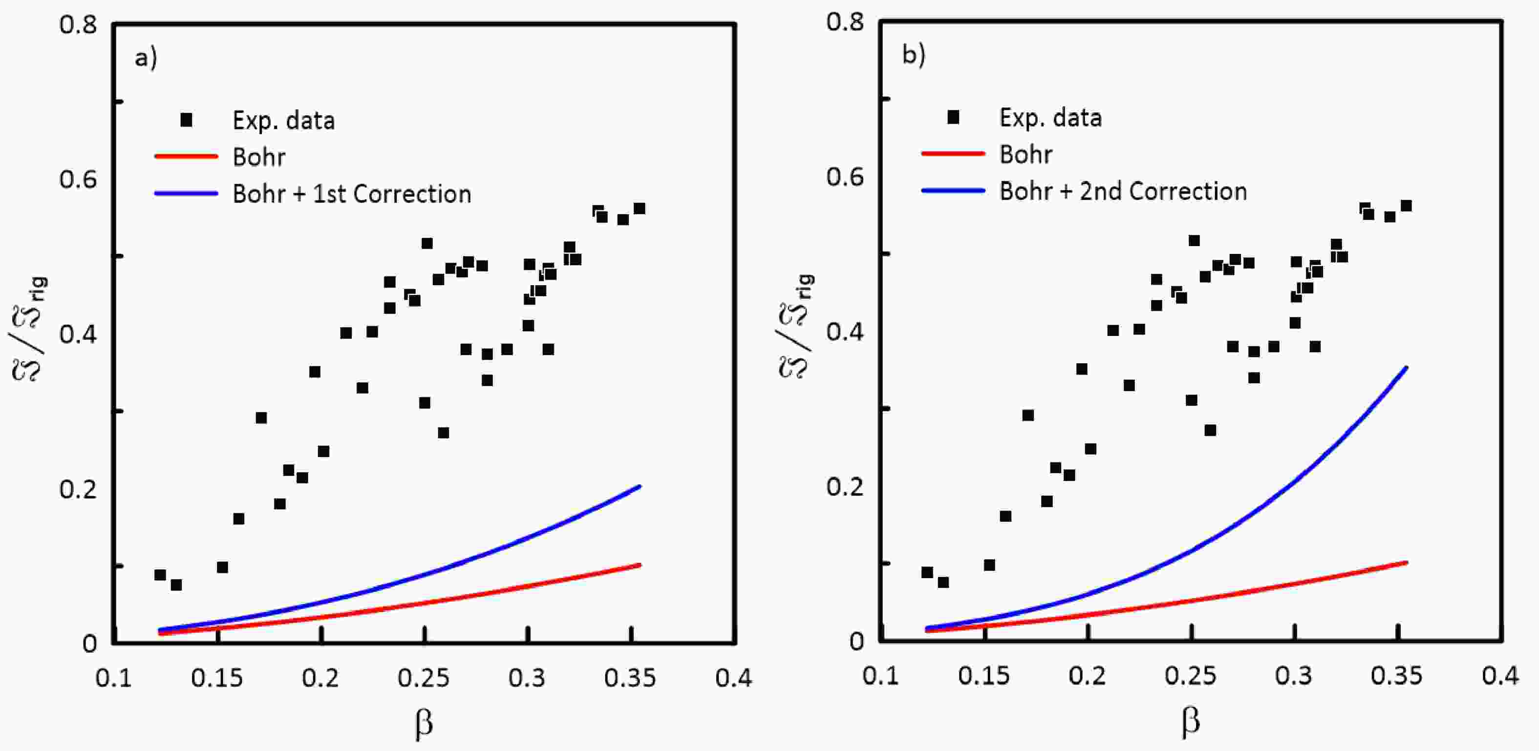
$ \beta $ deformation coefficients, which are extracted from the associated electric quadrupole transitions [22]. The third column presents the experimental values of$ MOI $ , which are deduced from the experimental energy spacing of the ground-state rotational bands [22]. The fourth, fifth, and sixth columns represent the calculated values using Eqs. (14), (21), and (30) to determine Bohr's ($ \Im_{k}^{\rm Bohr} $ ) first- ($ \Im' $ ) and second- ($ \Im{''} $ ) order modifications to the MOI, respectively. The seventh column presents the total MOI value obtained from Eq. (36), as$ \Im_{k}^{\rm Total} = \Im_{k}^{\rm Bohr}+\Im_{k}'+\Im_{k}{''} $ . All values of the MOI,$ \Im_{k} $ , in Table 1 are presented in units of$ \Im_{\rm rig} = B_{\rm rig}(1+0.31\beta) $ , where$B_{\rm rig} = 0.0138 A^{5/3} \hbar^2/{\rm MeV}$ and$ \Im_{\rm rig} $ is the MOI for a rigid body having the same volume, shape, and density of the nucleus. One can see from Table 1 that there is a large enhancement in the calculated values of$ \Im_{k}^{\rm Total} $ . It is equal to$ 0.6 $ in the case of the experimental ones instead of$ 0.2 $ in the case of the unmodified ones. It is remarkable to note that the second modification ($ \Im{''} $ ) to the MOI contributes$ \frac{250}{4\pi}\beta^2 $ times more than the Bohr value ($ \Im^{\rm Bohr} $ ). On the other hand, the first modification ($ \Im' $ ) is quite negligible. These phenomena are depicted clearly in Fig. 1a) and b); Fig 1a) depicts only the contribution of the first modification.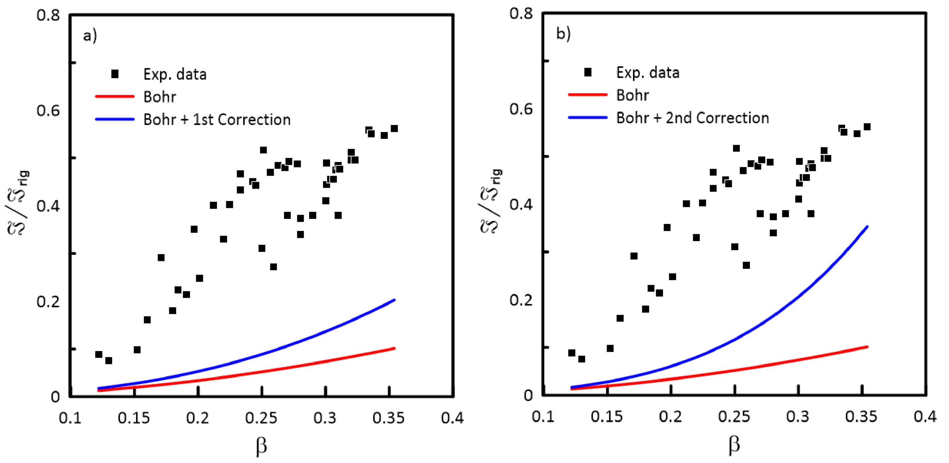
Figure 1. (color online) Variation of
$\Im/\Im_{\rm rig}$ with respect to deformation parameter$\beta$ for axially deformed nuclei: a) Bohr + first and b) Bohr + second modifications.Nuclei $\beta$ 

$\Im^{\exp.}$ 

$\Im^{\rm {Bohr}}$ 

$\Im'$ 

$\Im{''}$ 

$\Im^{\rm {Total}}$ 

$^{152}{\rm Sm}$ 

0.290 0.380 0.069 0.018 0.116 0.203 $^{154}{\rm Sm}$ 

0.336 0.551 0.092 0.028 0.206 0.325 $^{154}{\rm Gd}$ 

0.280 0.373 0.065 0.016 0.101 0.182 $^{156}{\rm Gd}$ 

0.320 0.498 0.083 0.024 0.170 0.277 $^{158}{\rm Gd}$ 

0.346 0.547 0.097 0.030 0.231 0.358 $^{160}{\rm Gd}$ 

0.354 0.561 0.101 0.032 0.252 0.385 $^{160}{\rm Dy}$ 

0.301 0.490 0.074 0.020 0.134 0.228 $^{162}{\rm Dy}$ 

0.320 0.512 0.083 0.024 0.170 0.277 $^{164}{\rm Dy}$ 

0.334 0.558 0.090 0.027 0.201 0.319 $^{164}{\rm Er}$ 

0.306 0.456 0.077 0.021 0.143 0.240 $^{166}{\rm Er}$ 

0.323 0.496 0.085 0.025 0.176 0.286 $^{168}{\rm Er}$ 

0.320 0.496 0.083 0.024 0.170 0.277 $^{170}{\rm Er}$ 

0.310 0.484 0.078 0.022 0.150 0.250 $^{170}{\rm Yb}$ 

0.304 0.455 0.076 0.021 0.139 0.235 $^{172}{\rm Yb}$ 

0.311 0.477 0.079 0.022 0.152 0.253 $^{174}{\rm Yb}$ 

0.308 0.475 0.078 0.022 0.146 0.245 $^{176}{\rm Yb}$ 

0.301 0.445 0.074 0.020 0.134 0.228 $^{176}{\rm Hf}$ 

0.300 0.410 0.074 0.020 0.132 0.226 $^{178}{\rm Hf}$ 

0.310 0.380 0.078 0.022 0.150 0.250 $^{180}{\rm Hf}$ 

0.270 0.380 0.060 0.015 0.087 0.162 $^{182}{\rm W}$ 

0.280 0.340 0.065 0.016 0.101 0.182 $^{184}{\rm W}$ 

0.250 0.310 0.052 0.012 0.065 0.128 $^{186}{\rm W}$ 

0.259 0.272 0.056 0.013 0.074 0.143 $^{186}{\rm Os}$ 

0.201 0.247 0.034 0.006 0.027 0.068 $^{188}{\rm Os}$ 

0.191 0.214 0.031 0.005 0.022 0.059 $^{190}{\rm Os}$ 

0.180 0.180 0.027 0.004 0.018 0.050 $^{192}{\rm Os}$ 

0.160 0.160 0.022 0.003 0.011 0.036 $^{194}{\rm Pt}$ 

0.152 0.097 0.020 0.003 0.009 0.032 $^{196}{\rm Pt}$ 

0.122 0.089 0.013 0.001 0.004 0.018 $^{198{\rm Pt}}$ 

0.130 0.076 0.015 0.002 0.005 0.021 Continued on next page Table 1. Comparison of calculated results
$\Im^{\rm Total}$ with experimental data$\Im^{\rm Exp.}$ [22] and$\Im_{\rm Hydro. model}^{\rm Bohr}$ as well as values of first$\Im'$ and second$\Im{''}$ modifications of${\rm MOI}$ for even-even axially deformed nuclei.Table 1-continued from previous page Nuclei $\beta$ 

$\Im^{\exp.}$ 

$\Im^{\rm{Bohr}}$ 

$\Im'$ 

$\Im{''}$ 

$\Im^{\rm{Total}}$ 

$^{222}{\rm Ra}$ 

0.184 0.223 0.029 0.005 0.019 0.053 $^{224}{\rm Ra}$ 

0.171 0.291 0.025 0.004 0.014 0.043 $^{226}{\rm Ra}$ 

0.197 0.351 0.033 0.006 0.025 0.064 $^{228}{\rm Ra}$ 

0.212 0.400 0.038 0.007 0.034 0.079 $^{226}{\rm Th}$ 

0.220 0.330 0.041 0.008 0.039 0.088 $^{228}{\rm Th}$ 

0.225 0.403 0.042 0.009 0.043 0.094 $^{230}{\rm Th}$ 

0.233 0.433 0.045 0.010 0.049 0.104 $^{232}{\rm Th}$ 

0.243 0.450 0.049 0.011 0.058 0.118 $^{234}{\rm Th}$ 

0.233 0.467 0.045 0.010 0.049 0.104 $^{230}{\rm U}$ 

0.245 0.443 0.050 0.011 0.060 0.121 $^{232}{\rm U}$ 

0.257 0.470 0.055 0.013 0.072 0.139 $^{234}{\rm U}$ 

0.251 0.516 0.052 0.012 0.066 0.130 $^{236}{\rm U}$ 

0.263 0.485 0.057 0.014 0.079 0.150 $^{238}{\rm U}$ 

0.268 0.480 0.059 0.014 0.085 0.159 $^{238}{\rm Pu}$ 

0.271 0.493 0.061 0.015 0.089 0.164 $^{240}{\rm Pu}$ 

0.278 0.488 0.068 0.018 0.111 0.196 aAll values of the moment of inertia are in terms of rigid body moment of inertia $\Im_{\rm{rig}}$ where

$\Im_{\rm{rig}} = (1+0.31\beta)B_{rig}$ and

$B_{\rm{rig} } = 0.0138A^{5/3}\frac{\hbar^2}{\rm{MeV} }.$ 

In order to illustrate the effects of the first and second corrections separately on Bohr's results, we draw a curve only for the first correction plus the values of Bohr and another curve for Bohr's values plus only the second correction (the orange curves in Fig. 1a) and b)); as functions of the deformation parameter
$ \beta $ .The graph includes curves for the original formula of Bohr and the experimental results for comparison. It is clear from this figure that for all
$ \beta\leqslant 0.15 $ , the effects of both of them are small enough to be neglected. As$ \beta >0.15 $ the contribution of the second correction increases more rapidly than that of the first one and it becomes greater than the zeroth order when$ \beta = 0.3 $ . This means that for nuclei with large deformation parameters, the assumption of small oscillations suggested by Rayleigh is not adequate. That means the first term is not enough to represent the situation of the nucleus.A comparison of the results obtained using the modified form of Bohr's relationship (the current work
$ \Im^{\rm Curr.} $ e), Eq. (34), and the results of Bohr's original relationship, Eq. (14), with the numerical calculations ($ \Im^{\rm Num.} $ ) presented by Berdichevsky et al. [9] as well as experimental data for a few nuclei are listed in Table 2. The numerical values were calculated based on the cranking model with the Sk-3 field.Nuclei $\beta$ [22]

$\Im^{\rm Exp.}$ 

$\Im^{\rm Num.}$ 

$\Im^{\rm Bohr}$ 

$\Im^{\rm Curr.}$ 

$^{154}{\rm Sm}$ 

0.336 36.59 24.54 6.20 21.91 $^{156}{\rm Gd}$ 

0.320 33.73 31.11 5.69 19.20 $^{158}{\rm Gd}$ 

0.346 33.73 29.88 7.84 25.26 $^{164}{\rm Dy}$ 

0.334 40.88 30.27 6.73 23.87 $^{166}{\rm Er}$ 

0.323 37.22 28.69 8.47 21.77 $^{168}{\rm Er}$ 

0.320 28.12 28.12 6.44 21.49 $^{174}{\rm Yb}$ 

0.308 39.22 31.13 7.13 20.09 Table 2. Comparison of values of
$\Im$ for some rare-earth even-even axially deformed nuclei (all values of$\Im$ in units$\hbar^{2} /{\rm MeV}$ ).Two features can be noted from Table 2:
i) In general, the results of the modified form of Bohr's relationship are much closer to the numerical results than of the original ones for all nuclei in question.
ii) The results of this work for the nuclei
$ ^{154}{\rm Sm} $ and$ ^{158}{\rm Gd} $ are close to the numerical ones (the ratio of the difference is nearly 8% for$ ^{154}{\rm Sm} $ and 16% for$ ^{158}{\rm Gd} $ , whereas it becomes large for the remaining nuclei). However, there are significant enhancements owing to the modification factor.The ratio
$ \Im /\Im_{\rm rig} $ with respect to$ \beta $ deformation for axially even-even deformed nuclei are illustrated in Fig. 2.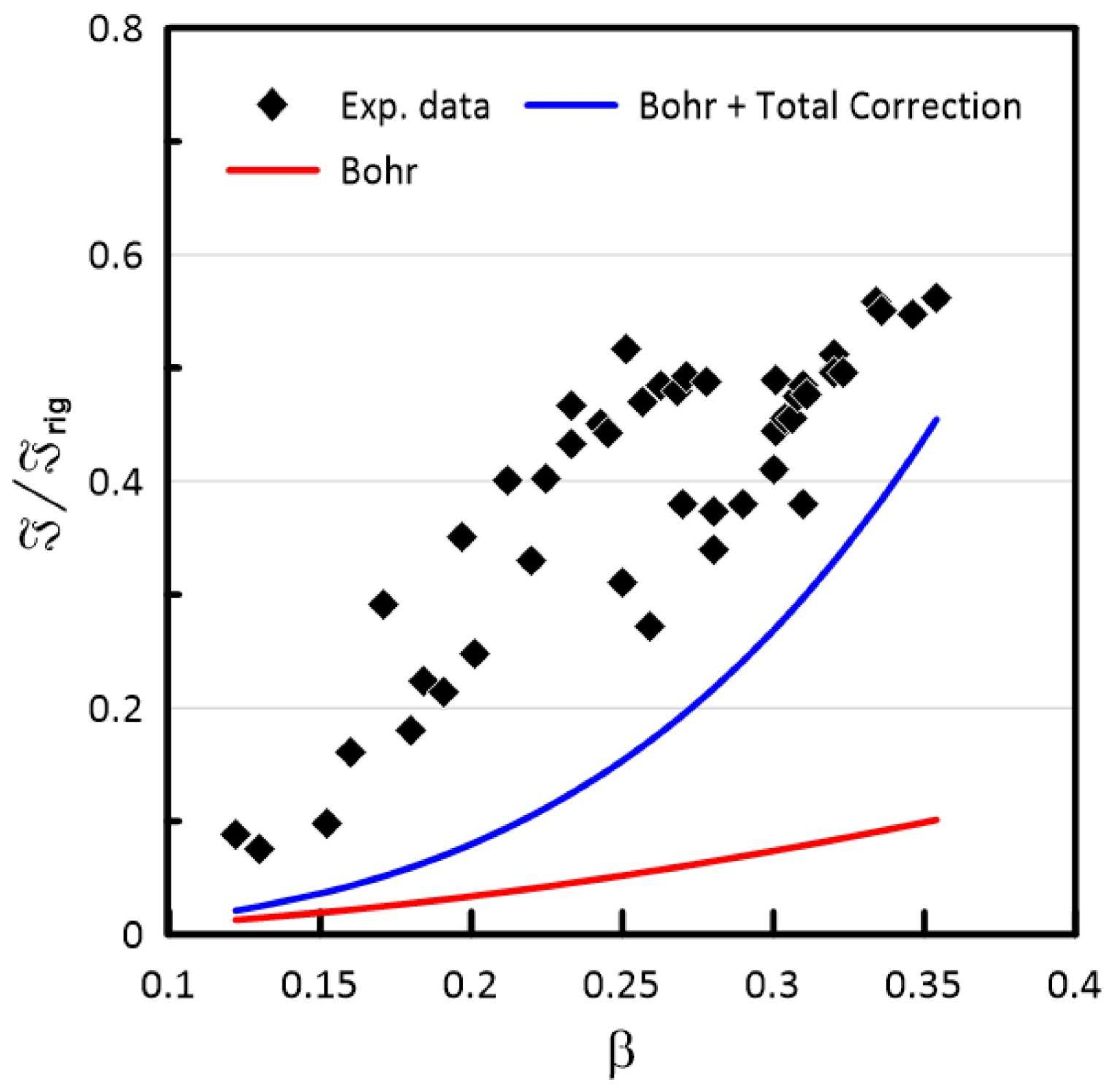
Figure 2. (color online) Variation of
$\Im/\Im_{rig}$ with respect to deformation parameter$\beta$ for axially deformed nuclei. Bohr + first + second modifications.The filled squares denote the experimental data, whereas the red line represents the
$ \Im^{\rm Bohr} $ values, which lie quite far from the experimental data [22]. Our results for Bohr + first modification and Bohr + second modification are represented with the blue line, which shifts towards the experimental data drastically. The shifting increases rapidly with an increase in$ \beta $ , mainly owing to the second modification to the MOI.For an average value of
$ \beta = 0.27 $ in the listed axially deformed nuclei, the Bohr estimates are only 18% of the experimental value, whereas the Bohr estimates with the first modification improve by 4%-5%, reaching 22%-23% of the experimental value. As soon as we include the second modification to this, the MOI values improve to beyond 53% of the experimental value. In mathematics, this occurs because of the symmetry properties of spherical harmonics. One can notice even number of$ Y_{2\mu} $ operators involved in the Bohr estimates and the second modification, whereas an odd number of$ Y_{2\mu} $ operators are involved in the first modification. Physically, it supports the large amplitude of vibrations at the nuclear surface for deformed rotating even-even nuclei. Further improvements have been predicted when a similar exercise is carried out for the next higher order terms, particularly with the next-to-next term having an even number of$ Y_{2} $ operators involved, which is going to be very complicated in nature and is in progress. Furthermore, we can obtain the total MOI in three coordinates for triaxial nuclei, as follows:$ \begin{split} \Im_{1}^{\rm Total} =& \Im^{\rm Bohr}_{1}+\Im_{1}'+\Im_{1}{''} \\ =& 4B\beta^2\sin^2\left(\gamma-\frac{2\pi}{3}\right) \left\{1+2C\sqrt{\frac{2}{7}}\beta\cos\gamma+\frac{250}{4\pi}\beta^2\right\} \\& -2CB\sqrt{\frac{2}{7}}\beta^3\cos\gamma\left(3\sqrt{3}\beta\sin\gamma+6\cos\gamma\right), \end{split} $

(37) $ \begin{split} \Im_{2}^{\rm Total} = & \Im^{\rm Bohr}_{2}+\Im_{2}'+\Im_{2}{''} \\ = & 4B\beta^2\sin^2\left(\gamma-\frac{4\pi}{3}\right) \left\{1+2C\sqrt{\frac{2}{7}}\beta\cos\gamma+\frac{250}{4\pi}\beta^2\right\} \\ & -2CB\sqrt{\frac{2}{7}}\beta^3\cos\gamma\left(-3\sqrt{3}\beta\sin\gamma+6\cos\gamma\right),\end{split} $

(38) $ \begin{split} \Im_{3}^{\rm Total} = & \Im^{\rm Bohr}_{3}+\Im_{3}'+\Im_{3}{''} \\ = & 4B\beta^2\sin^2(\gamma) \left\{1+2C\sqrt{\frac{2}{7}}\beta\cos\gamma+\frac{250}{4\pi}\beta^2\right\}, \end{split} $

(39) where we have used Eqs. (10), (11), and (12) to calculate the Bohr values of the MOI, represented as
$ \Im^{\rm Bohr}_{1}, \Im^{\rm Bohr}_{2}, \Im^{\rm Bohr}_{3} $ , respectively. The first modifications to the MOI are obtained using Eqs. (25), (26), and (27), respectively, and Eq. (34) is used for the second-order modification to the MOI.The total MOI,
$ \Im_{k}^{\rm Total} $ , for the triaxial nuclei has been calculated using Eqs. (37), (38), and (39). A comparison of the calculated results with the experimental data and Bohr estimation$ \left(\Im^{\rm Bohr}\right) $ is presented in Table 3. All the experimental values for the moments of inertia$ \Im_1, \Im_2, \Im_3 $ along the$ 1- $ ,$ 2- $ , and$ 3- $ body axes, respectively, as well as the deformation parameters$ \left(\beta,\gamma\right) $ have been acquired from Allmond and Wood [28]. Our calculated results are clearly in better agreement with the experimental data as compared to the original Bohr estimation.$A$ 

$\beta$ 

$\gamma$ 

$\Im_{1}^{\rm Exp.}$ 

$\Im^{\rm Bohr}_{1}$ 

$\Im^{\rm Total}_{1}$ 

$^{110}{\rm Ru}$ 

0.283 29.0 22.0 3.33 9.164 $^{150}{\rm Nd}$ 

0.283 10.4 27.5 4.96 13.982 $^{156}{\rm Gd}$ 

0.330 7.9 55.0 6.97 23.952 $^{166}{\rm Er}$ 

0.346 9.2 42.2 8.65 31.660 $^{168}{\rm Er}$ 

0.345 8.4 42.6 8.67 31.666 $^{172}{\rm Yb}$ 

0.331 4.9 38.3 7.88 27.281 $^{182}{\rm W}$ 

0.241 10.0 35.9 4.94 11.602 $^{184}{\rm W}$ 

0.234 11.3 30.6 4.82 10.955 $^{186}{\rm Os}$ 

0.207 20.4 32.4 4.16 8.286 $^{188}{\rm Os}$ 

0.193 19.9 26.5 3.67 6.872 $^{190}{\rm Os}$ 

0.184 22.1 24.1 3.44 6.163 $A$ 

$\beta$ 

$\gamma$ 

$\Im_{2}^{\rm Exp.}$ 

$\Im^{\rm Bohr}_{2}$ 

$\Im^{\rm Total}_{2}$ 

$^{110}{\rm Ru}$ 

0.283 29.0 8.1 0.88 2.540 $^{150}{\rm Nd}$ 

0.283 10.4 19.8 3.24 9.307 $^{156}{\rm Gd}$ 

0.330 7.9 21.2 5.05 17.609 $^{166}{\rm Er}$ 

0.346 9.2 33.3 5.94 22.096 $^{168}{\rm Er}$ 

0.345 8.4 33.6 6.16 22.818 $^{172}{\rm Yb}$ 

0.331 4.9 37.9 6.46 22.567 $^{182}{\rm W}$ 

0.241 10.0 25.7 3.28 7.852 $^{184}{\rm W}$ 

0.234 11.3 24.1 3.03 7.034 $^{186}{\rm Os}$ 

0.207 20.4 16.3 1.74 3.587 $^{188}{\rm Os}$ 

0.193 19.9 15.1 1.57 3.044 $^{190}{\rm Os}$ 

0.184 22.1 11.7 1.32 2.459 $A$ 

$\beta$ 

$\gamma$ 

$\Im_{3}^{\rm Exp.}$ 

$\Im^{\rm Bohr}_{3}$ 

$\Im^{\rm Total}_{3}$ 

$^{110}{\rm Ru}$ 

0.283 29.0 3.88 0.783 1.858 $^{150}{\rm Nd}$ 

0.283 10.4 1.96 0.18 0.427 $^{156}{\rm Gd}$ 

0.330 7.9 1.78 0.15 0.440 $^{166}{\rm Er}$ 

0.346 9.2 2.64 0.25 0.778 $^{168}{\rm Er}$ 

0.345 8.4 2.52 0.21 0.656 $^{172}{\rm Yb}$ 

0.331 4.9 1.39 0.07 0.202 $^{182}{\rm W}$ 

0.241 10.0 1.64 0.17 0.328 $^{184}{\rm W}$ 

0.234 11.3 2.31 0.21 0.388 $^{186}{\rm Os}$ 

0.207 20.4 2.78 0.52 0.873 $^{188}{\rm Os}$ 

0.193 19.9 3.45 0.44 0.692 $^{190}{\rm Os}$ 

0.184 22.1 4.08 0.50 0.754 Table 3. Comparison of calculated results of total MOI with experimental data [28] and Bohr estimates
$\Im^{\rm Bohr}$ for triaxial nuclei, respectively. -
A detailed theoretical extension to the hydrodynamical model has been presented in view of the contributions arising from the higher order terms of the radial distribution. Such calculated MOI values are found to be in better agreement than the original model for both axially deformed and triaxial nuclei. This highlights the crucial approximation involved in the irrotational picture of the liquid droplet in terms of small amplitude vibrations and further supports the large amplitude vibrations at the nuclear surface. Such investigations strengthen the irrotational and collective picture of even-even deformed nuclei. Further improvements to this extension are in progress.
It should be mentioned that the real value of
$ \xi_{2\mu}^{*} $ , which is presented in Section 3, is$\xi_{2\mu}^{*} = \dfrac{R_{0}}{2R}\dot{\alpha}_{2\mu}^{*}$ . This quantity was approximated by Rayleigh to$\dfrac{1}{2}\dot{\alpha}_{2\mu}^{*}$ by setting$ R = R_{0} $ . Another modification can be carried out here by expanding up to$ R $ and then treating the higher terms.In the future, we plan to predict the values of the parameters of inertia and rigidity within the hydrodynamic model using a simple harmonic potential.
The results obtained are compared with the experimental data as well as with Bohr's results and indicate good agreement with the experimental data, with ratios up to approximately 0.6 to sometimes 0.7.
We thank Prof. Ph.N. Usmanov, Prof. Dr. Abdul Kariem Bin HJ Mohd Arof, and all members of the Department of Science and Engineering for discussions that were very useful in improving our calculations. We also thank the MOHE, Fundamental Research Grant Scheme, FRGS19–039–0647 as well as OT~F2~2017/2020 by the Committee for the Coordination of the Development of Science and Technology under the Cabinet of Ministers of the Republic of Uzbekistan for supporting this research.
Prediction of moment of inertia of rotating nuclei
- Received Date: 2020-05-23
- Available Online: 2020-11-01
Abstract: In this study, the mathematical expression formulated by Bohr for the moment of inertia of even-even nuclei based on the hydrodynamical model is modified. The modification pertains to the kinetic energy of the surface oscillations, including the second and third terms of the R-expansion as well as the first term, which had already been modified by Bohr. Therefore, this work can be considered a continuation and support of Bohr's hydrodynamic model. The procedure yields a Bohr formula to be multiplied by a factor that depends on the deformation parameter. Bohr's (modified) formula is examined by applying it on axially symmetric even-even nuclei with atomic masses ranging between 150 and 190 as well as on some triaxial symmetry nuclei. In this paper, the modification of Bohr's formula is discussed, including information about the stability of this modification and the second and third terms of the R-expansion in Bohr's formula. The results of the calculation are compared with the experimental data and Bohr's results recorded earlier. The results obtained are in good agreement with experimental data, with a ratio of approximately 0.7, and are better than those of the unmodified ones.


 DownLoad: