


 Abstract
 HTML
HTML Reference
 Related
 PDF
PDF


-
Recently, the direct observation of gravitational waves by the LIGO-Virgo collaboration marked the coming of a new era of astronomical observation [1]. With the data of gravitational waves, the parameters of a black hole, such as the mass and spin, can be determined. It is expected that with improvement of the detection precision, further details of black holes and gravitational theories will be revealed.
It is widely known that in the last stage of a merged black hole, the ringdown modes can be described well by the quasinormal modes (QNMs). These modes are complex numbers, and can be regarded as the perturbations of a black hole in a given spacetime. To investigate the characteristic properties of a black hole using gravitational waves, one first needs to determine what is directly linked to the gravitational waves or QNMs. There are different approaches for calculating QNMs, aiming to reveal the characteristic properties of black holes [2-10].
Meanwhile, after the discovery of the four laws [11-14], black hole thermodynamics continues to be one of the most interesting subjects in black hole physics. A Schwarzschild black hole has only one thermodynamic phase of negative heat capacity, indicating that the isolated black hole is thermodynamically unstable. However, when the black hole obtains other hairs, such as the electric charge and spin, besides the negative heat phase, a phase of positive heat capacity will occur. Across these two black hole phases, the sign of the heat capacity of the black hole changes. More intriguingly, the heat capacity goes to infinity at the joined point of these two phases. This behavior may indicate a phase transition of the black hole system between the thermodynamically unstable and stable phases. Davies [15-17] found that this second order thermodynamic phase transition only takes place at the singular point of the heat capacity.
Additionally, the relation between the phase transition and QNMs has been studied [18-21]. Subsequently, Jing and Pan [22] proposed a clear relation between them stating that for a given quantum number beyond some certain critical value, the QNMs of a Reissner-Nordström (RN) black hole take on a spiral-like shape in the complex QNM plane when the Davies point is approached. Further, they found that both the real and imaginary parts of the QNMs behave as oscillatory functions of the black hole charge. However, Berti and Cardoso [23] argued that this result is probably a numerical coincidence due to the fact that it cannot be generalized to other black hole backgrounds. Whereas, He et al. [24] applied the study to a charged Kaluza-Klein black hole with a squashed horizon. They found that the existence of the spiral-like shape, and its starting point was consistent with the Davies point within 8%, or even lower for some other cases. These results imply that the relation between black hole thermodynamics and dynamics is nontrivial. Some other relevant works can be found in Refs. [25-27]
Due to the complexity of QNMs, only the numerical result is available, and an analytical investigation method for the relation is still lacking. According to the light ring/QNMs correspondence [28], the QNMs can be parametrized by the radius of the photon sphere in spherically symmetric spacetime, or the radius of the light ring in stationary spacetime. Moreover, this method is only effective in the eikonal limit, where the quantum numbers must have large values. It is interesting that this condition naturally satisfies the requirement of Ref. [22] where the quantum numbers must be larger than some critical values. Thus, using this light ring/QNMs correspondence, we can analytically check the relation given in Ref. [22], which is the main purpose of this paper. Several years ago, this correspondence was also applied to establish a universal relation between the QNMs and black hole lensing for asymptotically flat black holes with or without spin [29, 30].
Moreover, we conducted a study that explored the relation between the photon sphere (light ring) and the Van der Waals-type phase transition [31] for a charged or rotating black hole in anti-dS (AdS) spacetime [32, 33]. For a charged AdS black hole, non-monotonic behaviors of the photon sphere radius and the minimum impact parameter when the pressure and temperature are below their critical values were found, and the behaviors disappear when the parameters exceed their critical values [32]. Therefore, such non-monotonic behaviors can reflect a small/large black hole phase transition. During a small/large black hole phase transition, the radius and the minimum impact parameter of the photon sphere suddenly change, and these changes can serve as the order parameters to describe the small/large black hole phase transition. More interestingly, there exists a universal critical exponent of
$ 1/2 $ for the changes of the radius and the minimum impact parameter near the critical point, that is also independent of the dimension of the spacetime [32]. Such a study was also generalized to a rotating Kerr-AdS black hole [33]. In addition, another new issue was examined, and the result shows that the temperature and pressure corresponding to the extremal points of the radius or the angular momentum of the light rings exactly agree with that of the metastable curves from the thermodynamic side. All studies confirm that there exists a relation between the null geodesics and small/large black hole phase transition in AdS spacetime. The correspondence of the phase transition and the time-like geodesics can also be found in Ref. [34].As the angular velocity and Lyapunov exponent of the photon sphere respectively correspond to the real and imaginary parts of the QNMs, in this paper, we mainly aim to explore the relation between the angular velocity, Lyapunov exponent, and the Davies phase transition point in a static and spherically symmetric spacetime. We expect that our study on this relation could provide a possible way to test black hole thermodynamics with the observation of gravitational waves.
The paper is organized as follows: In Sec. 2, we briefly review the null geodesics and photon sphere for a black hole in a static and spherically symmetric spacetime. In Sec. 3, we calculate the Davies point and the photon sphere from the null geodesics for a four-dimensional, charged RN black hole. Then, we analytically obtain the angular velocity and Lyapunov exponent, and further explore the relation between the QNMs and the Davies point, as proposed in Ref. [22]. Unfortunately, the relation does not exactly hold. However, we propose a new and exact relation between the Davies point and the maximum of the temperature. Following this, we extend the study to a higher dimensional spacetime in Sec. 4. It is surprising that the spiral-like shape does not appear in the higher spacetime. Nevertheless, our new relation is still effective. In Sec. 5, we apply the study to a charged RN black hole in dS spacetime and obtain some novel results. Finally, the conclusions are presented in Sec. 6.
-
In a
$ d(\geqslant 4) $ -dimensional, static, and spherically symmetric spacetime, a black hole can be described by the following equation:$ {\rm d}s^{2} = -f(r){\rm d}t^{2}+\frac{1}{f(r)}{\rm d}r^{2}+r^{2}{\rm d}\Omega_{(d-2)}^{2}, $

(1) where
${\rm d}\Omega_{(d-2)}^{2}$ is the line element on a unit$ (d-2) $ -dimensional sphere$ S^{(d-2)} $ . The usual angular coordinates are$ \theta_{i}\in [0,\;\pi] $ $ (i = 1,\cdots,d-3) $ and$ \phi\in [0,\;2\pi] $ . The metric function$ f(r) $ depends on the radial coordinate r and other black hole parameters, such as the mass and charge.Next, the motion of a free photon in a black hole background is examined. As the spacetime here is spherically symmetric, without loss of generality, one can consider the motion limited in the equatorial hyperplane (
$ \theta_{i} = \dfrac{\pi}{2} $ for$ i = 1,\cdots ,d-3 $ ). Then, the Lagrangian for a photon reads$ 2{\cal{L}} = -f(r)\dot{t}^{2}+\dot{r}^{2}/f(r)+r^{2}\dot{\phi}^{2}. $

(2) The dot over a symbol denotes the ordinary differentiation with respect to an affine parameter. With the help of this Lagrangian, the generalized momentum defined by
$ p_{\mu} = \frac{\partial {\cal{L}}}{\partial \dot{x}^{\mu}} = g_{\mu\nu}\dot{x}^{\nu} $ has the following form$ p_{t} = -f(r)\dot{t}\equiv -E, $

(3) $ p_{\phi} = r^{2}\dot{\phi}\equiv l, $

(4) $ p_{r} = \dot{r}/f(r). $

(5) For this spacetime, there are two killing fields
$ \partial_{t} $ and$ \partial_{\phi} $ . Thus, there are two conservation constants E and l corresponding to each geodesics, which are the energy and orbital angular momentum of the photon, respectively. The t-motion and$ \phi $ -motion can be easily obtained by solving Eqs. (3) and (4),$ \dot{t} = \frac{E}{f(r)}, $

(6) $ \dot{\phi} = \frac{l}{r^{2}}. $

(7) The Hamiltonian for this system reads
$ \begin{split} 2{\cal{H}}\; & = 2(p_{\mu}\dot{x}^{\mu}-{\cal{L}})\\ & = -f(r)\dot{t}^{2}+\dot{r}^{2}/f(r)+r^{2}\dot{\phi}^{2}\\ & = -E\dot{t}+l\dot{\phi}+\dot{r}^{2}/f(r) = 0. \end{split} $

(8) Using the t-motion and
$ \phi $ -motion, it is easy to obtain the radial r-motion, which can be expressed in the following form$ \dot{r}^{2}+V_{\rm{eff}} = 0, $

(9) where the effective potential is
$ V_{\rm{eff}} = \frac{l^{2}}{r^{2}}f(r)-E^{2}. $

(10) As
$ \dot{r}^{2}> $ 0, the photon can only appear at the region of negative potential. A photon coming from infinity will fall into the black hole if it has low angular momentum. Meanwhile, for the larger angular momentum case, it will be bounded back to infinity when it meets a turning point determined by$ V_{\rm{eff}} = 0 $ . Among these two cases, there exists a critical case in which the photon traveling from infinity plunges into a circular orbit and will orbit the black hole in a closed loop. Nevertheless, such an orbit is unstable. Due to the spherical symmetry of the spacetime, such a circular orbit is known as the photon sphere. The conditions to determine this photon sphere are$ V_{\rm{eff}} = 0,\quad \frac{\partial V_{\rm{eff}}}{\partial r} = 0,\quad \frac{\partial^{2} V_{\rm{eff}}}{\partial r^{2}}<0. $

(11) The first two conditions can determine the radius
$ r_{\rm{ps}} $ and the critical angular momentum$ l_{\rm{ps}} $ of the photon sphere, while the third guarantees that the photon sphere is unstable.Substituting the effective potential (10) into the second condition, we obtain the equation that the radius
$ r_{\rm{ps}} $ must satisfy$ 2f(r_{\rm{ps}})-r_{\rm{ps}}\partial_{r}f(r_{\rm{ps}}) = 0. $

(12) For a given metric function
$ f(r) $ , we can obtain$ r_{\rm{ps}} $ by solving the equation. Then, from the first condition, the critical angular momentum can be obtained as$ u_{\rm{ps}} = \frac{l_{\rm{ps}}}{E} = \frac{r}{\sqrt{f(r)}}\bigg|_{r_{\rm{ps}}}. $

(13) The third condition is also closely linked to the QNMs of the black hole. Without loss of generality, we set E = 1.
Now, we consider the QNMs. In the eikonal limit (
$ l\gg1 $ ), the QNMs$ \omega_{\rm{Q}} $ can be calculated with the property of the photon sphere [28, 35, 36]$ \omega_{\rm{Q}} = l\Omega-{\rm i}\left(n+\frac{1}{2}\right)|\lambda|, $

(14) where n and l are the number of the overtone and the angular momentum of the perturbation, respectively. Here, we would like to emphasize that our calculation and discussion in this paper mainly depend on this relation, hence our result is only accurate in the eikonal limit. The other two quantities
$ \Omega $ and$ \lambda $ are the angular velocity and Lyapunov exponent of the photon sphere, respectively, which can be parameterized by the null geodesics$ \Omega = \frac{\dot{\phi}}{\dot{t}}\bigg|_{r_{\rm{ps}}},\quad \lambda = \sqrt{-\frac{V_{\rm{eff}}''}{2\dot{t}^{2}}}\bigg|_{r_{\rm{ps}}}. $

(15) Note that
$ V_{\rm{eff}}''|_{r_{\rm{ps}}}<0 $ , and the term under the square root is positive. In the background of (1), these two quantities can be expressed as$ \begin{split}& \Omega = \frac{\sqrt{f_{\rm{ps}}}}{r_{\rm{ps}}} = \frac{1}{l_{\rm{ps}}},\\& \lambda = \sqrt{\frac{f_{\rm{ps}}(2f_{\rm{ps}}-r^{2}_{\rm{ps}}f_{\rm{ps}}'')}{2r_{\rm{ps}}^{2}}}, \end{split}$

(16) where we have used (12). For a given metric function, one can easily obtain
$ \Omega $ and$ \lambda $ . Taking a Schwarzschild black hole as an example, we have$ r_{\rm{ps}} = 3M $ and$ l_{\rm{ps}} = 3\sqrt{3}M $ , which gives$ \Omega = 1/3\sqrt{3}M $ and$ \lambda = 1/3\sqrt{3}M $ . Although this method is effective for large l, it is still accurate for some cases with small l [10, 37].Following Refs. [28, 38], we would like to briefly comment on the relation between the QNMs in the eikonal limit and null geodesics. It is well known that in the eikonal limit, the scalar, electromagnetic, and gravitational perturbations in the background (1) have the same behavior, so we take the scalar perturbation as an example, which obeys the Klein-Gordon equation. By employing the method of the separation of variables, the radial partial wave function
$ \Phi_{l}(r) $ satisfies the Regge-Wheeler equation$ \frac{{\rm d}^{2}\Phi_{l}}{{\rm d}r_{*}^{2}}-V_{l}\Phi_{l} = 0, $

(17) where the convenient “tortoise” coordinate
$ r_{*} $ ranges from$ -\infty $ to$ +\infty $ . The potential$ V_{l}(r) $ reads$\begin{split} V_{l}(r) =\; & \frac{l(l+d-3)}{r^{2}}f(r)+\frac{(d-2)(d-4)}{4r^{2}}f^{2}(r)\\ &+\frac{d-2}{2r}f(r)f'(r)-\omega^{2}, \end{split} $

(18) where
$ \omega $ is the frequency of the perturbation and can correspond to the energy$ E = \hbar \omega $ of the perturbation particle. In the eikonal limit$ l\gg1 $ , the second and third terms on the right-hand side of (18) can be ignored, and$ l(l+d-3)\approx l^{2} $ ; thus, the potential reduces to$ V_{l}(r) = \frac{l^{2}}{r^{2}}f(r)-\omega^{2}. $

(19) It is clear that these two potentials in (10) and (19) are the same, as well as the equation of motion. Therefore, it is reasonable to obtain the QNMs following the null geodesics method. It is worth noting that this method cannot be extended to asymptotically AdS spacetime.
-
The four-dimensional charged RN black hole solution is given by equation (1) with the following function
$ f(r) = 1-\frac{2M}{r}+\frac{Q^{2}}{r^{2}}. $

(20) The parameters M and Q are the mass and charge of the black hole, respectively. Solving
$ f(r) = 0 $ , the outer and inner horizons of the black hole can be easily obtained, which are located at$ r_{\pm} = M\pm\sqrt{M^{2}-Q^{2}}. $

(21) The entropy and temperature corresponding to the event horizon are
$ S = \pi (M+\sqrt{M^{2}-Q^{2}})^{2}, $

(22) $ T = \frac{M^{2}-Q^{2}+M\sqrt{M^{2}-Q^{2}}} {2\pi(M+\sqrt{M^{2}-Q^{2}})^{3}}. $

(23) The heat capacity at a fixed charge is
$\begin{split} C_{Q} \;&= T\left(\frac{{\rm d}S}{{\rm d}T}\right)_{Q} = \frac{2S(S-\pi Q^{2})}{3\pi Q^{2}-S} \\ &= \frac{2\pi(M+\sqrt{M^{2}-Q^{2}})^{2}((M+\sqrt{M^{2}-Q^{2}})^{2}-Q^{2})}{3 Q^{2}-(M+\sqrt{M^{2}-Q^{2}})^{2}}.\end{split}$

(24) We plot the heat capacity
$ C_{Q} $ in Fig. 1. It is clear that when the charge is small,$ C_{Q} $ is negative just like for a Schwarzschild black hole, indicating that the black hole is thermodynamically unstable. Meanwhile, for the large charge case,$ C_{Q} $ becomes positive and the black hole is thermodynamically stable. Among these two cases, the heat capacity diverges at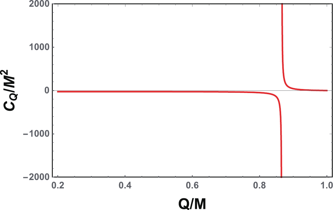
Figure 1. (color online) Heat capacity
$C_{Q}$ vs. Q for the four-dimensional charged RN black hole. The heat capacity diverges at$Q_{\rm{D}}/M=\dfrac{\sqrt{3}}{2}$ .$ Q_{\rm{D}} = \frac{\sqrt{3}}{2}M\approx0.8660M, $

(25) which is called the Davies point. It was shown by Davies [15-17] that this divergence point measures a phase transition of the black hole between the thermodynamically unstable and stable phases.
-
In Ref. [22], Jing and Pan explored the Davies point using the QNMs. They proposed that when a black hole passes through this phase transition point, the QNMs in the complex
$ \omega_{Q} $ plane begin to take a spiral-like shape, and both the real and imaginary parts of the QNMs for a given overtone number and angular quantum number beyond the critical values become the oscillatory functions of the black hole charge. This provides an interesting dynamic to study the thermodynamic phase transition. However, in Ref. [23], Cardoso et al. argued that this result is probably a numerical coincidence. Nevertheless, this relation between the thermodynamic and dynamic properties of black holes was further confirmed in Ref. [24]. In the following, we would like to analytically examine this relation in detail in the eikonal limit.As shown in Ref. [22], the relation holds for a large overtone number n and small l. In our approach, we extend this study to the eikonal limit to check whether the relation holds. For a charged black hole, the radius of the photon sphere can be obtained by solving (12)
$ r_{\rm{ps}} = \frac{1}{2} \left(3M+\sqrt{9 M^2-8 Q^2}\right). $

(26) For the case of
$ Q = 0 $ , we have$ r_{\rm{ps}} = 3M $ for the Schwarzschild black hole. For the extremal charged black hole$ Q = M $ , the photon sphere will be located at$ r = 2M $ . Substituting$ r_{\rm{ps}} $ into (16), we obtain the angular velocity and Lyapunov exponent of the photon sphere$ \Omega = \frac{1}{3M+\sqrt{9M^{2}-8Q^{2}}}\sqrt{2+\frac{M(\sqrt{9M^{2}-8Q^{2}}-3M)}{2Q^{2}}}, $

(27) $ \lambda = \frac{4\sqrt{\begin{aligned}\left(M(3M+\sqrt{9M^{2}-8Q^{2}})-2Q^{2}\right) \left(3M(3M+\sqrt{9M^{2}-8Q^{2}})-8Q^{2}\right)\end{aligned}}}{\left(3M+\sqrt{9M^{2}-8Q^{2}}\right)^{3}}. \quad\quad\quad$

(28) Note that in Ref. [22], the authors studied this issue by fixing the mass, i.e.,
$ 2M = 1 $ ; here, we will rescale all these quantities with the black hole mass, which is equivalent to settin M = 1. In the small charge limit and for a fixed mass, we have$ \Omega M \sim \frac{1}{3\sqrt{3}}+\frac{1}{18\sqrt{3}}\left(\frac{Q}{M}\right)^2+{\cal{O}}\left(\frac{Q}{M}\right)^4, $

(29) $ \lambda M \sim \frac{1}{3\sqrt{3}}+\frac{1}{54\sqrt{3}}\left(\frac{Q}{M}\right)^2+{\cal{O}}\left(\frac{Q}{M}\right)^4. $

(30) The study of Ref. [28] showed that the spiral-like shape exists in the complex
$ \omega_{Q} $ plane when the Davies point is passed. As$ \Omega $ and$ \lambda $ respectively correspond to the real and imaginary parts of QNMs, here, we would like to discuss the corresponding result in the$ \Omega $ -$ \lambda $ plane by varying the charge$ Q/M $ . The result is given in Fig. 2. Apparently, with the increase of the charge$ Q/M $ , the spiral-like shape will appear at a certain value of$ Q/M $ . For clarity, we plotted the angular velocity$ \Omega M $ (top red line) and Lyapunov exponent$ \lambda M $ (bottom blue line) as a function of the charge$ Q/M $ , as shown in Fig. 3. Interestingly,$ \Omega M $ is a monotonically increasing function of$ Q/M $ . However,$ \lambda M $ first slowly increases with the charge and approaches its maximum at a certain value of$ Q/M $ , then decreases. Therefore, no oscillatory exists for$ \Omega M $ or$ \lambda M $ , which is different from that of Refs. [10, 22]. The reason for this might result from the fact that we consider the case in the eikonal limit, while in Refs. [10, 22], the case with small l and a higher overtone number n was considered. Moreover, the non-monotonic behavior of$ \lambda M $ shown in Fig. 3 is closely linked to the starting point of the spiral-like shape. Therefore, this point can be determined by the maximum of$ \lambda M $ . After a simple calculation, we determine the point as
Figure 2. (color online) Angular velocity and Lyapunov exponent in the
$\Omega$ -$\lambda$ plane. The black arrow indicates the increase of the charge$Q/M$ .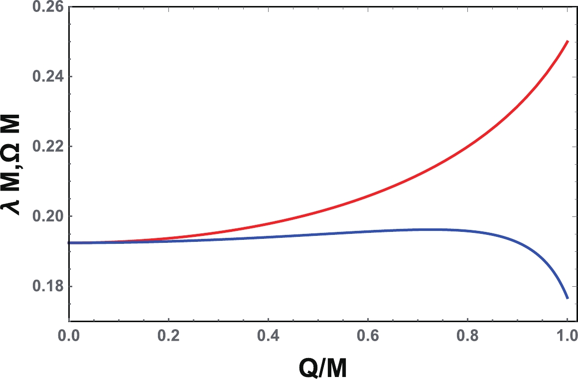
Figure 3. (color online) Angular velocity
$\Omega M$ (top red line) and the Lyapunov exponent$\lambda M$ (bottom blue line) as functions of the charge$Q/M$ .$ Q_{\rm{S}}/M = \frac{\sqrt{51-3\sqrt{33}}}{8}\approx0.7264. $

(31) Hence, the starting point of the spiral-like shape is smaller than the Davies point given in (25). The deviation between them is approximately 16%. It is worth noting that the starting point occurs at the value of the charge at which the real part of the oscillatory quasinormal frequencies arrives at its maximum, with the different critical overtone number
$ n_c $ [22].In summary, for the charged RN black hole, the Davies point and the starting point of the spiral-like shape are not the same. Thus, the relation proposed in Ref. [22] cannot be exactly extended to the eikonal limit. Nevertheless, the spiral-like shape can reflect the existence of the thermodynamic phase transition or Davies point. Moreover, we note that the black hole with charge
$ Q_{\rm{S}} $ (31) is characterized by the fastest relaxation rate among all the charged RN black holes [39]. -
As shown above, the relation given in Ref. [22] is approximate. Here, we would like to examine whether a new precise relation exists.
Our recent work [32, 33] showed the existence of a relation between the black hole's null geodesics and the thermodynamic phase transition of a liquid/gas type in AdS spacetime. Motivated by this, we expected to apply it to a charged RN black hole to investigate the relation between null geodesics and the Davies point.
From (26), we can express the black hole mass with the radius of the photon sphere as
$ M = \frac{2Q^{2}+r_{\rm{ps}}^{2}}{3r_{\rm{ps}}}. $

(32) Substituting this into (23), the temperature will be of the form
$ T = \frac{3r_{\rm{ps}}\sqrt{(r_{\rm{ps}}^{2}-Q^{2})(r_{\rm{ps}}^{2}-4Q^{2})}\left(\sqrt{(r_{\rm{ps}}^{2}-Q^{2})(r_{\rm{ps}}^{2}-4Q^{2})}+(2Q^{2}+r_{\rm{ps}}^{2})\right)}{2\pi \left(8Q^{4}-Q^{2}r_{\rm{ps}}^{2}+2r_{\rm{ps}}^{4}+2(2Q^{2}+r_{\rm{ps}}^{2})\sqrt{(r_{\rm{ps}}^{2}-Q^{2})(r_{\rm{ps}}^{2}-4Q^{2})}\right)^{3/2}}. $

(33) In terms of
$ r_{\rm{ps}} $ and Q, the angular velocity and the Lyapunov exponent are$ \Omega = \frac{\sqrt{r_{\rm{ps}}^{2}-Q^{2}}}{\sqrt{3}r_{\rm{ps}}^{2}}, $

(34) $ \lambda = \frac{\sqrt{(r_{\rm{ps}}^{2}-Q^{2})(r_{\rm{ps}}^{2}-2Q^{2})}}{\sqrt{3}r_{\rm{ps}}^{3}}. $

(35) In Fig. 4, the temperature T is plotted as a function of
$ \Omega $ and$ \lambda $ , respectively. From Figs. 4(a) and 4(b), the temperature behaviors are seen to be similar. At first, the temperature increases with$ \Omega $ or$ \lambda $ . After its maximum is approached, it decreases. Therefore, there are two different black hole phases bounded by the maximum of the temperature. In the last subsection, we showed that the Lyapunov exponent has a peak at a certain charge. This behavior is quite similar to that of Fig. 4(b). Thus, there must exist a characteristic charge corresponding to the maximum temperature. Next, we will calculate this charge. At the maximum temperature, the parameters have the following values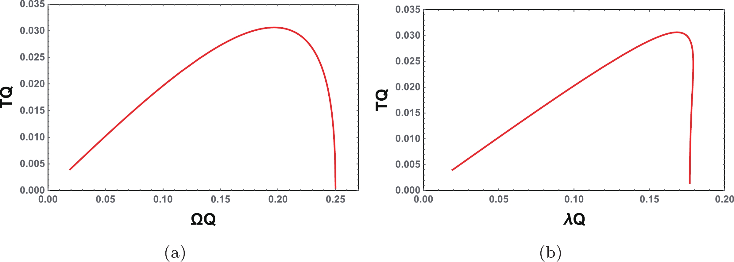
Figure 4. (color online) (a) T vs.
$\Omega$ , (b) T vs.$\lambda$ for the four-dimensional charged RN black hole.$\begin{split} & T_{\rm{M}} = \frac{1}{6\sqrt{3}\pi Q},\quad \Omega_{\rm{M}} = \frac{1}{2Q}\sqrt{\frac{2\sqrt{3}}{3}-1},\\ & \lambda_{\rm{M}} = \frac{1}{2Q}\sqrt{3-\frac{5}{\sqrt{3}}}. \end{split}$

(36) Correspondingly, the radius of the photon sphere for this case is
$ r_{\rm{psM}} = (1+\sqrt{3})Q. $

(37) Finally, using (26), we obtain the point corresponding to the maximum of the temperature
$ Q_{\rm{M}} = \frac{\sqrt{3}}{2}M. $

(38) It is clear that this point exactly matches the Davies point (25), where the heat capacity diverges. It is close to the point (31) with only a small difference.
In summary, we established a new relation between the black hole thermodynamics and dynamics. The phase transition point or Davies point is exactly located at the maximum in the T-
$ \Omega $ or T-$ \lambda $ plane. This may provide us a new dynamic way to precisely probe the Davies point. -
For a d-dimensional charged black hole, the line element is in the same form of (1), while the metric function is given by
$ f(r) = 1-\frac{m}{r^{d-3}}+\frac{q^{2}}{r^{2(d-3)}}. $

(39) The parameters m and q are linked to the black hole mass M and charge Q as
$ m = \frac{16\pi M}{(d-2)A_{d-2}}, \quad $

(40) $ q = \frac{8\pi Q}{\sqrt{2(d-2)(d-3)A_{d-2}}}, $

(41) where
$ A_{d-2} = 2\pi^{(d-1)/2}/\Gamma\left((d-1)/2\right) $ is the area of the unit (d-2) sphere. The horizons located at the roots of$ f(r) = 0 $ $ r_{\pm}^{d-3} = \frac{1}{2}\left(m\pm\sqrt{m^{2}-4q^{2}}\right). $

(42) Similar to the four-dimensional case, the higher-dimensional black hole has two horizons for
$ q/m<\frac{1}{2} $ , one horizon for$ q/m = \frac{1}{2} $ , or no horizon for$ q/m>\frac{1}{2} $ . The temperature and entropy corresponding to the outer horizon are$ T = \frac{(d-3)(r_{+}^{2d}-q^{2}r_{+}^{6})}{4\pi r_{+}^{2d+1}}, $

(43) $ S = \frac{A_{d-2}r_{+}^{d-2}}{4}. $

(44) The heat capacity at fixed charge Q is
$ C_{Q} = \frac{A_{d-2}(d-2)(r_{+}^{2d}-q^{2}r_{+}^{6})} {4(2d-5)q^{2}r_{+}^{8-d}-4 r_+^{d+2}}. $

(45) The behavior of this heat capacity is similar to that in the four-dimensional black hole case. For small charge,
$ C_{Q} $ is negative, while for large charge,$ C_{Q} $ becomes positive. Moreover,$ C_{Q} $ diverges at$ q^{2} = \frac{r_{+}^{2(d-3)}}{2d-5}. $

(46) We list the Davies points in Table 1 for d = 5–10.
d=5 d=6 d=7 d=8 d=9 d=10 $Q_{\rm{D}}/M$ 

0.8607 0.8101 0.7589 0.7136 0.6744 0.6404 $Q_{\rm{M}}$ /M

0.8607 0.8101 0.7589 0.7136 0.6744 0.6404 $r_{\rm{psM}}/Q^{\frac{1}{d-3}}$ 

1.3189 1.1085 1.0497 1.0361 1.0410 1.0547 $T_{\rm{M}}Q^{\frac{1}{d-3}}$ 

0.1404 0.2552 0.3593 0.4528 0.5373 0.6146 $\Omega_{\rm{M}}Q^{\frac{1}{d-3}}$ 

0.5240 0.6916 0.7735 0.8130 0.8301 0.8349 $\lambda_{\rm{M}}Q^{\frac{1}{d-3}}$ 

0.6897 1.1478 1.5033 1.7806 2.0017 2.1820 Table 1. Davies points and parameter values corresponding to the maximum value of the temperature
$T_{\rm{M}}$ for higher-dimensional charged Reissner-Nordström black holes.Solving (12), we can obtain the radius of the photon sphere
$ r_{\rm{ps}}^{d-3} = \frac{4\pi}{(d-2)A_{d-2}}\left((d-1)M+ \sqrt{(d-1)^{2}M^{2}-\frac{2(d-2)^{2}Q^{2}}{d-3}}\right). $

(47) Moreover, the angular velocity and Lyapunov exponent are
$ \Omega^{2} = \frac{1+q^{2}r_{\rm{ps}}^{6-2d}-mr_{\rm{ps}}^{3-d}}{r_{\rm{ps}}^{2}}, $

(48) $ \lambda^{2} = \frac{(q^{2}r_{\rm{ps}}^{6}+r_{\rm{ps}}^{2d}-mr_{\rm{ps}}^{d+3})(2r_{\rm{ps}}^{2d} -2(d-2)(2d-7)q^{2}r_{\rm{ps}}^{6}+(d-1)(d-4)mr_{\rm{ps}}^{d+3})}{2r_{\rm{ps}}^{2(2d+1)}}. $

(49) In Fig. 5, we show the angular velocity and Lyapunov exponent in the
$ \Omega $ -$ \lambda $ plane for the spacetime dimension d = 5–10, respectively. Different from the d = 4 case, no spiral-like shapes exist for the higher-dimensional black hole cases, and the angular velocity$ \Omega $ is just a monotonically decreasing function of$ \lambda $ . To further understand this result, the behaviors of the angular velocity and Lyapunov exponent are presented in Fig. 6 as functions of the black hole charge. Apparently,$ \Omega $ increases while$ \lambda $ decreases with charge Q. Both of these are monotonic functions of Q. Therefore, the spiral-like shape does not exist for the higher-dimensional charged black holes. Meanwhile, we note that in Ref. [24], for a five-dimensional charged Kaluza-Klein black hole with squashed horizons, the QNMs were found to demonstrate spiral-like shapes near the Davies point, which may be caused by the non-vanishing Kaluza-Klein parameters.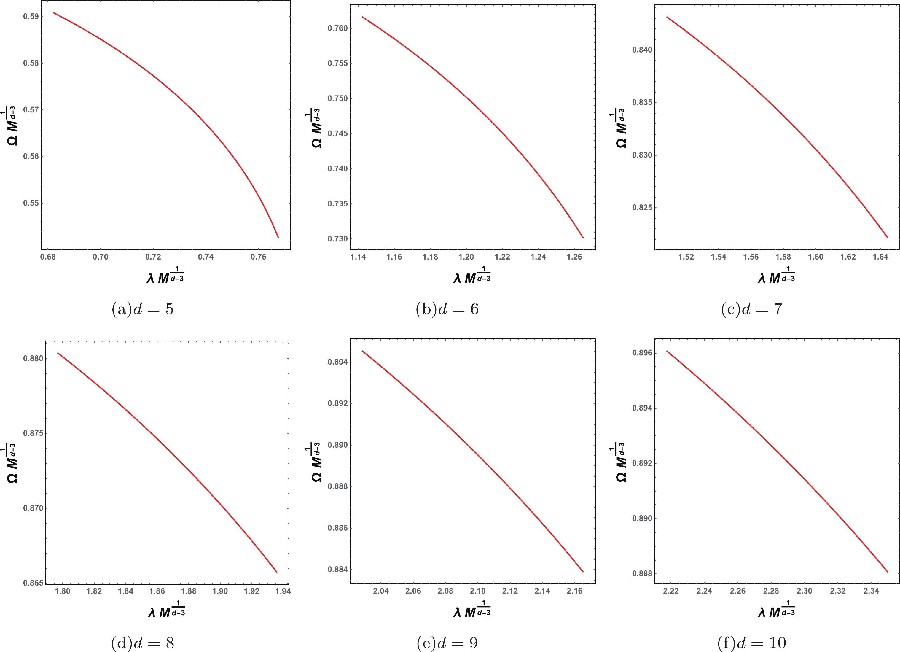
Figure 5. (color online) Angular velocity
$\Omega$ and Lyapunov exponent$\lambda$ in the$\Omega$ -$\lambda$ plane. The black hole charge Q increases from bottom right to top left. The maximum bound of the charge is 1,$\dfrac{2}{\sqrt{3}}$ ,$\sqrt{\dfrac{3}{2}}$ ,$2\sqrt{\dfrac{2}{5}}$ ,$\sqrt{\dfrac{5}{3}}$ ,$2\sqrt{\dfrac{3 }{7}}$ , and$\dfrac{\sqrt{7}}{2}$ respectivelyfor (a) d = 5, (b) d = 6, (c) d = 7, (d) d = 8, (e) d = 9, (f) d = 10.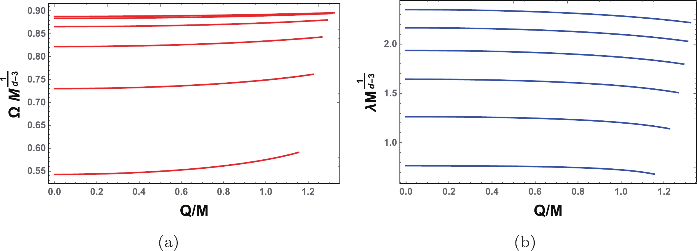
Figure 6. (color online) Behaviors of the angular velocity and Lyapunov exponent as functions of the black hole charge. Spacetime dimension d=5–10 from bottom to top. (a)
$\Omega$ vs. Q; (b)$\lambda$ vs. Q.In the above section, we presented a new relation between the black hole thermodynamics and dynamics for the four-dimensional spacetime. The temperature has a maximum value in the T-
$ \Omega $ or T-$ \lambda $ plane, and the maximum point is found to correspond to the Davies point. Here, we speculate if this property holds for higher-dimensional spacetime. To answer this question, we describe the temperature T as a function of$ \Omega $ and$ \lambda $ , respectively, as shown in Fig. 7. Interestingly, similar to the four-dimensional case, maximum values for the temperature are also exhibited in both the figures for d = 5–10. Using these maximum values of the temperature, we can obtain the corresponding charge$ Q_{\rm{M}} $ . The parameter values corresponding to the maximum values of the temperature are listed in Table 1 for d = 5–10. From the table, we can clearly see that the Davies points and the$ Q_{\rm{M}} $ exactly match each other for d = 5–10. Thus, we can confirm that the relation proposed above also holds for the higher-dimensional black holes.
Figure 7. (color online) (a) T vs.
$\Omega$ ; (b) T vs.$\lambda$ ; Spacetime dimension d=5–10 from bottom to top. -
Recently, there has been a great focus on the strong cosmic censorship in dS spacetime [40-49]. Many works have shown that this censorship may be violated for a charged RN-dS black hole by calculating the QNMs of different types of perturbations. In particular, in Ref. [40], the authors divided the QNMs for the charged RN-dS black hole into three families: the photon sphere modes, dS modes, and near-extremal modes. Therefore, it is very interesting to examine the relation presented in the above section by calculating the angular velocity and the Lyapunov exponent of the photon sphere modes.
Here, we only consider the four-dimensional spacetime. The charged RN-dS black hole solution is also described by equation (1) with the function
$ f(r) = 1-\frac{2M}{r}+\frac{Q^{2}}{r^{2}}-\frac{\Lambda}{3}r^{2}. $

(50) Here, the parameter
$ \Lambda $ is the cosmological constant, which is positive for dS spacetime. For this case, there exists a cosmological horizon outside the event horizon, and both can be obtained by solving$ f(r) = 0 $ . Moreover, we can express the mass M with the radius$ r_{+} $ of the event horizon$ M = \frac{3Q^{2}+3r_{+}^{2}-r_{+}^{4}\Lambda}{6r_{+}}. $

(51) The black hole entropy corresponding to the event horizon is still a quarter of its area
$ S = A/4 = \pi r_{+}^{2} $ . Thus, the mass can be further expressed as$ M = \frac{3\pi^{2} Q^{2}+3\pi S-S^{2}\Lambda}{6\pi^{3/2}S^{1/2}}. $

(52) Similarly, the temperature of the event horizon is
$ T = \frac{-\pi^{2}Q^{2}+\pi S-S^{2}\Lambda}{4(\pi S)^{3/2}}. $

(53) The heat capacity at fixed charge Q and cosmological
$ \Lambda $ is$ C_{Q,\Lambda} = \frac{2S(\pi^{2}Q^{2}-\pi S+S^{2}\Lambda)}{-3\pi^{2}Q^{2}+\pi S+S^{2}\Lambda}. $

(54) Note that
$ C_{Q,\Lambda} $ exactly vanishes at T = 0, which corresponds to the extremal black hole case. Further, it diverges at the point where its denominator vanishes, i.e.,$ S = \frac{\pi(\sqrt{1+12Q^{2}\Lambda}-1)}{2\Lambda}. $

(55) This is just the Davies point. Substituting into Eq. (52), we can find another form of the Davies point
$ \Lambda M^{2} = \frac{2}{9}\left(\sqrt{12Q^{2}\Lambda+1}-1\right), $

(56) or
$ \left(\frac{Q_{\rm{D}}}{M}\right)^{2} = \frac{3}{4}+\frac{27}{16}\Lambda M^{2}. $

(57) It is clear that when the cosmological constant
$ \Lambda\rightarrow0 $ , this result will reduce back to that of the RN black hole case (25). It is worth noting that this Davies point (57) is different from that given in [17], where the coefficient of the second term on the right side of the corresponding equation is$ \dfrac{81}{16} $ , not$ \dfrac{27}{16} $ . The reason for this is that Davies made a change of$ \Lambda\rightarrow 3\Lambda $ . Thus, both results are consistent with each other.Now, we consider the null geodesics for a charged dS black hole. By solving (12), we obtain the radius of the photon sphere,
$ r_{\rm{ps}} = \frac{1}{2}\left(3M+\sqrt{9M^{2}-8Q^{2}}\right). $

(58) Interestingly, this result is of the form in (26) for the asymptotically flat case without the cosmological constant. The reason for this is not hard to understand. From (10), we can find that the cosmological constant
$ \Lambda $ term only comes to the effective potential as a constant. The photon sphere is obtained by solving$ \partial_{r}V_{\rm{eff}} = 0 $ , so after the derivation, the effect of$ \Lambda $ in the metric function$ f(r) $ disappears, resulting in the same form of the photon sphere as in the asymptotically flat case. Nevertheless, it should be considered that the mass M here depends on the cosmological constant, see Eq. (52).Adopting the form of (58), we can further obtain the angular velocity and the Lyapunov exponent,
$ \Omega = \frac{\sqrt{-9 M^2 \left(4 \Lambda Q^2+1\right)+3 M \sqrt{9 M^2-8 Q^2} \left(1-4 \Lambda Q^2\right)+4 Q^2 \left(4 \Lambda Q^2+3\right)}}{\sqrt{6} Q \left(\sqrt{9 M^2-8 Q^2}+3 M\right)}, $

(59) $\lambda \!= \!\frac{4 \sqrt{8 Q^2\!-\!3 M \left(\sqrt{9 M^2-8 Q^2}+3 M\right)}}{\sqrt{3} \left(\sqrt{9 M^2\!-\!8 Q^2}\!+\!3 M\right)^3} \sqrt{ 81 \Lambda M^4\!-\!9 M^2 \left(8 \Lambda Q^2+1\right)\!+\!3 M \sqrt{9 M^2\!-\!8 Q^2} \left(9 \Lambda M^2\!-\!4 \Lambda Q^2-1\right)+8 \Lambda Q^4\!+\!6 Q^2}.$

(60) In addition, we plotted the behavior of the angular velocity and Lyapunov exponent in the
$ \Omega $ -$ \lambda $ plane for$ \Lambda M^{2} $ = 0.01, 0.05, and 0.1, as shown in Fig. 8. For fixed$ \Lambda M^{2} $ , it is clear that there exist spiral-like shapes in this plane, similar to the asymptotically flat case. The existence of the spiral-like shapes also indicates the nonmonotonic behavior of$ \lambda $ rather than$ \Omega $ . For clarity, these are shown in Fig. 9. The values of the charge at the starting point of the spiral-like shapes for$ \Lambda M^{2} $ = 0.01, 0.05, and 0.1 are$ Q_{\rm{S}}/M $ = 0.7684, 0.8862, and 0.9716, respectively, which are different from the Davies points$ Q_{\rm{D}}/M $ = 0.8757, 0.9134, and 0.9585. Therefore, the result clearly shows that the starting points of the spiral-like shapes and the Davies points do not match.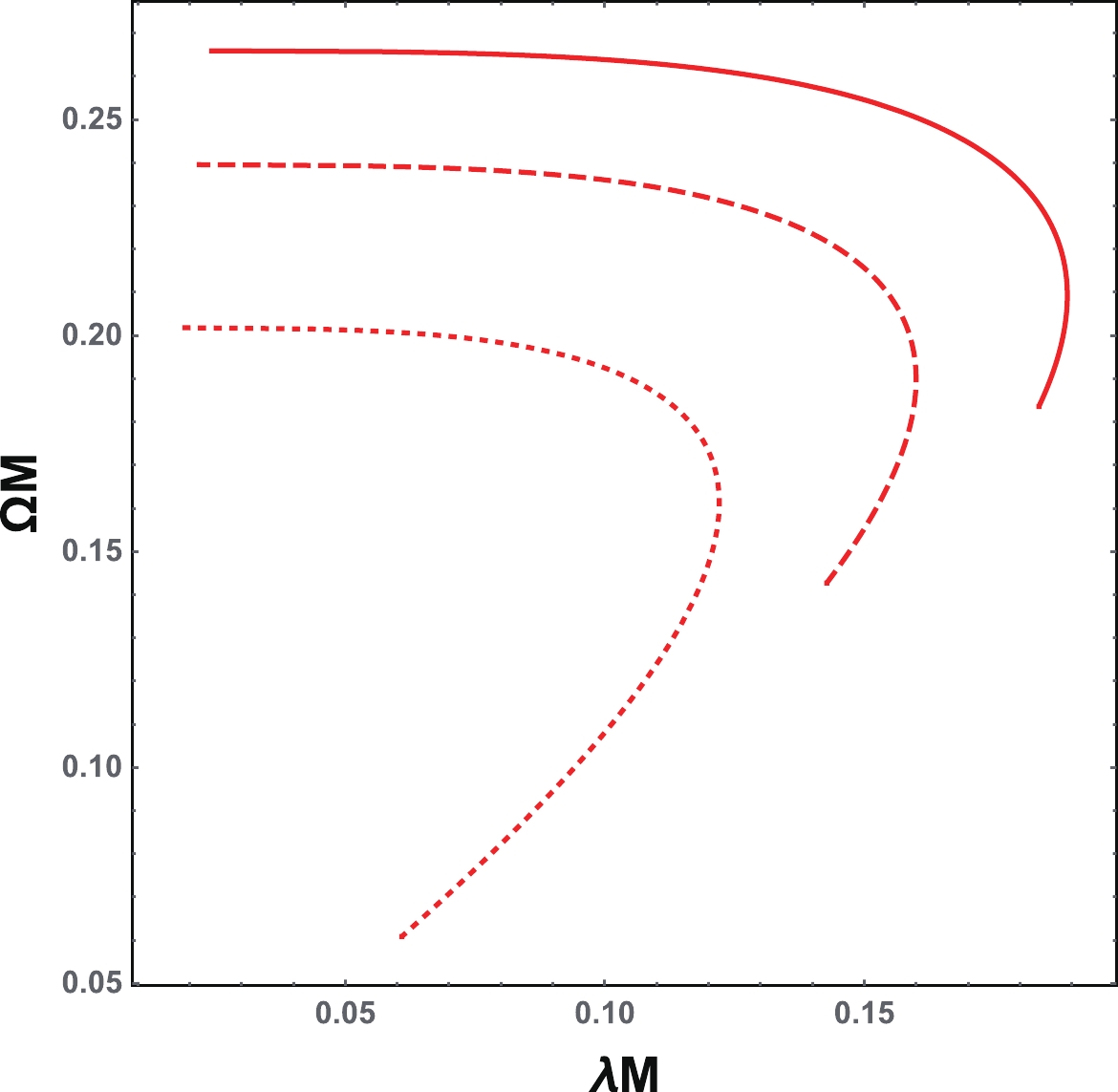
Figure 8. (color online) Angular velocity and Lyapunov exponent in the
$\Omega$ -$\lambda$ plane for$\Lambda M^{2}$ = 0.01 (solid line), 0.05 (dashed line), and 0.1 (dotted line) for the charged RN-dS black hole.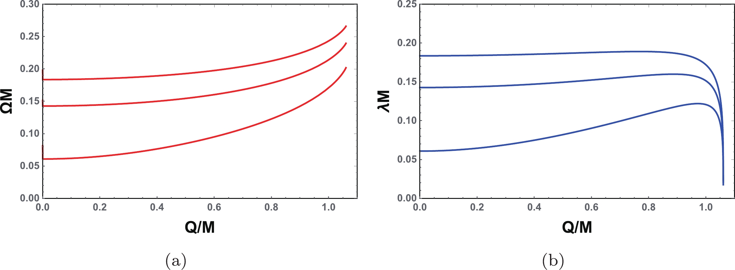
Figure 9. (color online) Behaviors of the angular velocity and Lyapunov exponent as functions of the black hole charge for
$\Lambda M^{2}$ =0.01, 0.05, and 0.1, respectively, from top to bottom.In Fig. 10, we describe the behavior of the temperature as a function of
$ \Omega $ and$ \lambda $ , respectively. From this, there is a local maximum for each fixed$ \Lambda Q^{2} $ . With the increase of$ \Lambda Q^{2} $ , the maximum decreases and is shifted to small value of$ \Omega $ or$ \lambda $ . Moreover, the values for different parameters corresponding to the maximum of the temperature are listed in Table 2. It is clear that the Davies point and starting point of the spiral-like shape are not consistent with each other. For small$ \Lambda $ ,$ Q_{\rm{S}} $ is smaller than$ Q_{\rm{D}} $ . However, with the increase of$ \Lambda $ ,$ Q_{\rm{S}} $ increases faster than$ Q_{\rm{D}} $ . For example, for$ \Lambda Q^{2} = 0.1 $ ,$ Q_{\rm{S}} $ will be larger than$ Q_{\rm{D}} $ . Meanwhile, the value of the charge$ Q_{\rm{M}} $ corresponding to the maximum exactly coincides with the Davies point$ Q_{\rm{D}} $ given in (57). Therefore, this further confirms our new relation between the black hole thermodynamics and dynamics shown in Sec. 3.3. In summary, this conjecture is not only effective for asymptotically flat spacetime, but also for asymptotically dS spacetime.$\Lambda Q^{2}$ =0.01

$\Lambda Q^{2}$ =0.05

$\Lambda Q^{2}$ =0.1

$Q_{\rm{D}}/M$ 

0.8786 0.9216 0.9650 $Q_{\rm{S}}$ /M

0.7906 0.9085 0.9774 $Q_{\rm{M}}$ /M

0.8786 0.9216 0.9650 $r_{\rm{psM}}/Q$ 

2.6639 2.4333 2.1996 $T_{\rm{M}}Q$ 

0.0293 0.0240 0.0176 $\Omega_{\rm{M}}Q$ 

0.1924 0.1736 0.1460 $\lambda_{\rm{M}}Q$ 

0.1631 0.1412 0.1118 Table 2. Charges of the Davies point and starting point of the spiral-like shape of the charged RN-dS black holes. The other parameter values correspond to the maximum value of the temperature
$T_{\rm{M}}$ .
Figure 10. (color online) Behaviors of the temperature T as a function of
$\Omega$ and$\lambda$ for$\Lambda Q^{2}$ = 0.01, 0.05, and 0.1 from top to bottom. (a) T-$\Omega$ ; (b) T-$\lambda$ -
In this paper, we focused on extending the relation first proposed in [22] to the eikonal limit between the spiral-like shape of the QNMs and the thermodynamic phase transition point, the Davies point.
For the four-dimensional charged RN black hole, a simple spiral-like behavior is exhibited in the
$ \Omega $ -$ \lambda $ plane. The reason for this is because the Lyapunov exponent$ \lambda $ has a maximum as the black hole charge Q changes. Meanwhile, the angular velocity$ \Omega $ is a monotonic increasing function of the black hole charge. This result is very different from the numerical results given in Ref. [22], where both$ \Omega $ and$ \lambda $ are non-monotonic functions of the charge, leading to an explicit spiral-like behavior in the$ \Omega $ -$ \lambda $ plane. Nevertheless, the authors claimed that the Davies point is linked to the starting point of this spiral-like shape. Their numerical result states that the difference between these two points is very small, indicating the existence of a correspondence. We also analytically examined this issue in detail and the result shows that the starting point of the spiral-like shape is$ Q_{\rm{S}} = \dfrac{\sqrt{51-3\sqrt{33}}}{8}M\approx0.7264M $ , which deviates by approximately 16% from the Davies point$ Q_{\rm{D}} = \dfrac{\sqrt{3}}{2}\approx0.8660M $ . Therefore, the Davies point and the starting point of the spiral-like shape do not exactly coincide in the eikonal limit. However, we further investigated the behavior of the black hole temperature as a function of the angular velocity and Lyapunov exponent. The temperature in both the figures clearly demonstrates a local maximum. More interestingly, the local maximum analytically coincides with the Davies point. This indicates that there is a relation between the Davies point and the maximum of the temperature in the T-$ \Omega $ and T-$ \lambda $ planes. As both$ \Omega $ and$ \lambda $ correspond to the QNMs of the black hole, this relation may provide an exact correspondence between the black hole thermodynamics and dynamics.In addition, we extended our investigation to the higher-dimensional spacetime. One interesting result different from the four-dimensional case is that, in the
$ \Omega $ -$ \lambda $ plane, the spiral-like shape does not exist. Therefore, the relation between the Davies point and the behavior of the spiral-like shape is completely lost. Fortunately, the proposed relation between the Davies point and the maximum of the temperature in the T-$ \Omega $ and T-$ \lambda $ planes still holds for higher-dimensional charged black holes.Moreover, we applied the study to a charged RN black hole in dS spacetime, and the results are similar to those of the asymptotically flat spacetime. The Davies point, the starting point of the spiral-like shape, and the maximum of the temperature in the T-
$ \Omega $ and T-$ \lambda $ planes were all found to increase with the cosmological constant. As expected, the Davies point and the starting point of the spiral-like shape do not coincide with each other. Meanwhile, the Davies point exactly coincides with the maximum of the temperature, which further confirms our new relation even in dS spacetime.Before ending this paper, we would like to provide a few comments. First, at least in the eikonal limit, there is no exact relation between the Davies point and the spiral-like shape of the QNMs. Second, there is a nontrivial and exact relation between the Davies point and the maximum of the temperature in the T-
$ \Omega $ and T-$ \lambda $ planes. Additionally, some other relations between the thermodynamics and dynamics are worth exploring beyond the eikonal limit.We would like to thank Profs. Qiyuan Pan and Robert B. Mann for the useful discussions.
Null geodesics, quasinormal modes, and thermodynamic phase transition for charged black holes in asymptotically flat and dS spacetimes
- Received Date: 2020-04-01
- Accepted Date: 2020-06-17
- Available Online: 2020-11-01
Abstract: A numerical study has indicated that there exists a relation between the quasinormal modes and the Davies point for a black hole. In this paper, we analytically study this relation for charged Reissner-Nordström black holes in asymptotically flat and de Sitter (dS) spacetimes in the eikonal limit, under which the quasinormal modes can be obtained from the null geodesics using the angular velocity


 DownLoad: