Decay properties of the Z_c(3900) through the Fierz rearrangement

In the past twenty years, many charmonium-like $ XYZ $ states have been discovered in particle experiments [1]. All of these are good multiquark candidates, and their relevant experimental and theoretical studies have significantly improved our understanding of the strong interaction at the low energy region. In particular, in 2013, BESIII reported the $ Z_c(3900)^+ $ in the $ Y(4260) \to J/\psi\pi^+\pi^- $ process [2], which was later confirmed by Belle [3] and CLEO [4]. Since it couples strongly to the charmonium and yet it is charged, the $ Z_c(3900)^+ $ is not a conventional charmonium state and contains at least four quarks. It is quite interesting to understand how it is composed of these four quarks, and there have been various models developed to explain this, such as a compact tetraquark state composed of a diquark and an antidiquark [5, 6], a loosely-bound hadronic molecular state composed of two charmed mesons [7-13], a hadro-quarkonium [8, 14, 15], or due to the kinematical threshold effect [16-19], etc. We refer to reviews [20-24] for detailed discussions.

The charged charmonium-like state $ Z_c(3900) $ of $ J^{PC} = 1^{+-} $ [25] has been observed in the $ J/\psi \pi $ and $ D \bar D^* $ channels [2, 3, 26, 27], and there were some events in the $ h_c \pi $ channel [28]. In a recent BESIII experiment [29], evidence for the $ Z_c(3900) \rightarrow \eta_c\rho $ decay was reported with a statistical significance of $ 3.9\sigma $ at $ \sqrt{s} = 4.226 $ GeV, and the relative branching ratio

was evaluated to be $ 2.2 \pm 0.9 $ at the same center-of-mass energy. This ratio has been studied by many theoretical methods/models [30-39], and was suggested in Ref. [40] to be useful to discriminate between the compact tetraquark and hadronic molecule scenarios. As summarized in Table 1, this ratio was calculated in many molecular models, but the extracted values are highly model dependent. Hence, it would be useful to derive a model-independent result, and it would be even better to do so within the same framework for both the tetraquark and molecule scenarios.

interpretations	${\cal{R}}_{Z_c}$	methods/models
compact tetraquark	$\left( 2.3^{+3.3}_{-1.4} \right) \times 10^2$	Type-I diquark-antidiquark model [40]
	$0.27^{+0.40}_{-0.17}$	Type-II diquark-antidiquark model [40]
	$0.95$	QCD sum rules [30]
	$0.57$	QCD sum rules [31]
	$1.1$	QCD sum rules [32]
	$1.28$	covariant quark model [33]
hadronic molecule	$\left( 4.6^{+2.5}_{-1.7} \right) \times 10^{-2}$	Non-Relativistic effective field theory [40]
	$0.12$	light front model [34]
	$0.68 \times 10^{-2}$	effective field theory [35]
	$1.78$	covariant quark model [33]

Table 1.  The relative branching ratio ${\cal{R}}_{Z_c} \equiv {\cal{B}}(Z_c(3900) \rightarrow \eta_c\rho) / {\cal{B}}(Z_c(3900) \rightarrow J/\psi\pi)$, calculated by various theoretical methods/models.

In this paper we study the decay properties of the $ Z_c(3900) $ under both the compact tetraquark and hadronic molecule interpretations. This study is based on our previous finding that the diquark-antidiquark currents ($ [qq][\bar q \bar q] $) and the meson-meson currents ($ [\bar q q][\bar q q] $) are related to each other through the Fierz rearrangement of the Dirac and color indices [41-51]. More studies on light baryon operators can be found in Refs. [52-54]. In the present case the $ Z_c(3900) $ contains four quarks: the c, $ \bar c $, q, $ \bar q $ quarks ($ q = u/d $). Thus, there are three configurations:

Again, the Fierz rearrangement can be applied to relate them. Based on these relations, we shall extract some decay properties of the $ Z_c(3900) $ in this paper.

There are eight independent $ [cq][\bar c \bar q] $ currents of $ J^{PC} = 1^{+-} $, which have been systematically constructed in Ref. [55]. Here, we choose one of them,

where $ {\mathbb{C}} $ is the charge-conjugation matrix, the subscripts $ a \cdots e $ are the color indices, and the sum over repeated indices is taken. This current would strongly couple to the $ Z_c(3900) $, if it has the same internal structure (internal symmetry) as that state.

The above current is useful from the viewpoints of both effective field theory and QCD sum rules. Note that there are various quark-based effective field theories, which have been successfully applied to describe the meson and baryon systems, such as the Non-Relativistic QCD for the heavy quarkonium system [56, 57]:

We refer to Ref. [58] for a detailed review of this method. The above Lagrangian contains four four-fermion operators, which can be used to study the annihilation width of a heavy quarkonium into light particles. In this method the Fierz rearrangement is applied to decouple the Dirac and color indices that connect the short-distance part to the long-distance part [57].

Compared with this, the quark-based effective field theory for the multiquark system is much more difficult [24]. Let us attempt to do this for the $ Z_c(3900) $. Based on Eq. (2), we can add an eight-quark operator (the same argument applies for other Lagrangians containing $ \eta^{{\cal{Z}}}_{\mu} $):

where $ c_0 $ is a constant. Next, we can use the Fierz rearrangement to transform it to

Detailed discussions on this transformation will be given below.

Considering that the meson operators, $ \bar q \gamma_5 q $, $ \bar q \gamma_{\mu} q $, $ \bar c \gamma_5 c $, and $ \bar c \gamma_{\mu} c $ couple to the $ \pi $, $ \rho $, $ \eta_c $, and $ J/\psi $ mesons (see Table 2 at Sec. 3), the above eight-quark operator can describe the fall-apart decays of the $ Z_c(3900) $ into the $ \eta_c \rho $ and $ J/\psi \pi $ final states simultaneously, together with some other possible decay channels. In order to extract the widths of these decays, one still needs to do further calculations, which we shall not examine further. However, their relative branching ratios can be extracted much more easily, which are useful and important for understanding the nature of the $ Z_c(3900) $ [59].

operators	$J^{PC}$	mesons	$J^{PC}$	couplings	decay constants
$J^{S} = \bar d u$	$0^{++}$	–	$0^{++}$	–	–
$J^{P} = \bar d i\gamma_5 u$	$0^{-+}$	$\pi^+$	$0^{-+}$	$\langle 0 | J^{P} | \pi^+ \rangle = \lambda_\pi$	$\lambda_\pi = \dfrac{f_\pi m_\pi^2}{m_u + m_d}$
$J^{V}_{\mu} = \bar d \gamma_{\mu} u$	$1^{–}$	$\rho^+$	$1^{–}$	$\langle 0 | J^{V}_{\mu} | \rho^+ \rangle = m_\rho f_{\rho^+} \epsilon_{\mu}$	$f_{\rho^+} = 208$ MeV [82]
$J^{A}_{\mu} = \bar d \gamma_{\mu} \gamma_5 u$	$1^{++}$	$\pi^+$	$0^{-+}$	$\langle 0 | J^{A}_{\mu} | \pi^+\rangle = {\rm i} p_{\mu} f_{\pi^+}$	$f_{\pi^+} = 130.2$ MeV [1]
		$a_1(1260)$	$1^{++}$	$\langle 0 | J^{A}_{\mu} | a_1 \rangle = m_{a_1} f_{a_1} \epsilon_{\mu} $	$f_{a_1} = 254$ MeV [87]
$J^{T}_{\mu\nu} = \bar d \sigma_{\mu\nu} u$	$1^{\pm-}$	$\rho^+$	$1^{–}$	$\langle 0 | J^{T}_{\mu\nu} | \rho^+ \rangle = {\rm i} f^T_{\rho} (p_{\mu}\epsilon_\nu - p_\nu\epsilon_{\mu})$	$f_{\rho}^T = 159$ MeV [82]
		$b_1(1235)$	$1^{+-}$	$\langle 0 | J^{T}_{\mu\nu} | b_1 \rangle = {\rm i} f^T_{b_1} \epsilon_{\mu\nu\alpha\beta} \epsilon^\alpha p^\beta$	$f_{b_1}^T = 180$ MeV [95]
$I^{S} = \bar c c$	$0^{++}$	$\chi_{c0}(1P)$	$0^{++}$	$\langle 0 | I^S | \chi_{c0} \rangle = m_{\chi_{c0}} f_{\chi_{c0}}$	$f_{\chi_{c0}} = 343$ MeV [76]
$I^{P} = \bar c i\gamma_5 c$	$0^{-+}$	$\eta_c$	$0^{-+}$	$\langle 0 | I^{P} | \eta_c \rangle = \lambda_{\eta_c}$	$\lambda_{\eta_c} = \dfrac {f_{\eta_c} m_{\eta_c}^2}{2 m_c}$
$I^{V}_{\mu} = \bar c \gamma_{\mu} c$	$1^{–}$	$J/\psi$	$1^{–}$	$\langle 0 | I^{V}_{\mu} | J/\psi \rangle = m_{J/\psi} f_{J/\psi} \epsilon_{\mu}$	$f_{J/\psi} = 418$ MeV [83]
$I^{A}_{\mu} = \bar c \gamma_{\mu} \gamma_5 c$	$1^{++}$	$\eta_c$	$0^{-+}$	$\langle 0 | I^{A}_{\mu} | \eta_c \rangle = {\rm i} p_{\mu} f_{\eta_c}$	$f_{\eta_c} = 387$ MeV [83]
		$\chi_{c1}(1P)$	$1^{++}$	$\langle 0 | I^{A}_{\mu} | \chi_{c1} \rangle = m_{\chi_{c1}} f_{\chi_{c1}} \epsilon_{\mu} $	$f_{\chi_{c1}} = 335$ MeV [77]
$I^{T}_{\mu\nu} = \bar c \sigma_{\mu\nu} c$	$1^{\pm-}$	$J/\psi$	$1^{–}$	$\langle 0 | I^{T}_{\mu\nu} | J/\psi \rangle = {\rm i} f^T_{J/\psi} (p_{\mu}\epsilon_\nu - p_\nu\epsilon_{\mu})$	$f_{J/\psi}^T = 410$ MeV [83]
		$h_c(1P)$	$1^{+-}$	$\langle 0 | I^{T}_{\mu\nu} | h_c \rangle = {\rm i} f^T_{h_c} \epsilon_{\mu\nu\alpha\beta} \epsilon^\alpha p^\beta$	$f_{h_c}^T = 235$ MeV [83]
$O^{S} = \bar d c$	$0^{+}$	$D_0^{*+}$	$0^{+}$	$\langle 0 | O^{S} | D_0^{*+} \rangle = m_{D_0^{*}} f_{D_0^{*}}$	$f_{D_0^{*}} = 410$ MeV [108]
$O^{P} = \bar d i\gamma_5 c$	$0^{-}$	$D^+$	$0^{-}$	$\langle 0 | O^{P} | D^+ \rangle = \lambda_D$	$\lambda_D = \dfrac{f_D m_D^2 }{{m_c + m_d}}$
$O^{V}_{\mu} = \bar c \gamma_{\mu} u$	$1^{-}$	$\bar D^{*0}$	$1^{-}$	$\langle 0 | O^{V}_{\mu} | \bar D^{*0} \rangle = m_{D^*} f_{D^*} \epsilon_{\mu}$	$f_{D^*} = 253$ MeV [105]
$O^{A}_{\mu} = \bar c \gamma_{\mu} \gamma_5 u$	$1^{+}$	$\bar D^{0}$	$0^{-}$	$\langle 0 | O^{A}_{\mu} | \bar D^{0} \rangle = {\rm i} p_{\mu} f_{D}$	$f_{D} = 211.9$ MeV [1]
		$D_1$	$1^{+}$	$\langle 0 | O^{A}_{\mu} | D_1 \rangle = m_{D_1} f_{D_1} \epsilon_{\mu} $	$f_{D_1} = 356$ MeV [108]
$O^{T}_{\mu\nu} = \bar d \sigma_{\mu\nu} c$	$1^{\pm}$	$\bar D^{*+}$	$1^{-}$	$\langle 0 | O^{T}_{\mu\nu} | D^{*+} \rangle = {\rm i} f_{D^*}^T (p_{\mu}\epsilon_\nu - p_\nu\epsilon_{\mu})$	$f_{D^*}^T \approx 220$ MeV
		–	$1^{+}$	–	–

Table 2.  Couplings of meson operators to meson states. Color indices are omitted for simplicity.

The current $ \eta^{{\cal{Z}}}_{\mu} $ can also be investigated from the viewpoint of QCD sum rules [60, 61]. We assume it couples to the $ Z_c(3900) $ through

After the Fierz rearrangement, $ \eta^{{\cal{Z}}}_{\mu} $ transforms to the long expression inside Eq. (5). Through the first and second terms, it couples to the $ \eta_c \rho $ and $ J/\psi \pi $ channels simultaneously:

Again, these two equations can be easily used to calculate the relative branching ratio $ {\cal{R}}_{Z_c} $. Detailed discussions on this will be given below.

In the above equations, we have worked within the naive factorization scheme, so our uncertainty is significantly larger than the well-developed QCD factorization method [62-64], which has been widely and successfully applied to study weak and radiative decay properties of conventional (heavy) hadrons, e.g., see Refs. [65, 66]. However, given that we still do not fully understand the internal structure of the $ Z_c(3900) $ (as well as all the other exotic hadrons), the naive factorization scheme at this moment can be useful. Besides, the tetraquark decay constant $ f_{Z_c} $ is removed when calculating relative branching ratios, which significantly reduces our uncertainty.

In this study, we shall examine the strong decay properties of the $ Z_c(3900) $ under the naive factorization scheme. To do this we just need to replace the weak-interaction Lagrangian by some interpolating current, and apply the similar technics here together with the Fierz arrangement. Note that a similar arrangement of the spin and color indices in the nonrelativistic case was used to study strong decay properties of the $ Z_c(3900) $ in Refs. [8, 67, 68].

This paper is organized as follows. In Sec. 2 we systematically construct all the tetraquark currents of $ J^{PC} = 1^{+-} $ with the quark content $ c \bar c q \bar q $. There are three configurations, $ [cq][\bar c \bar q] $, $ [\bar c q][\bar q c] $, and $ [\bar c c][\bar q q] $, and their relations are also derived in this section by using the Fierz rearrangement of the Dirac and color indices. In Sec. 3 we discuss the couplings of meson operators to meson states and list those which are needed in the present study. In Sec. 4 and Sec. 5 we extract some decay properties of the $ Z_c(3900) $, separately for the compact tetraquark interpretation and the hadronic molecule interpretation. The obtained results are discussed and summarized in Sec. 6.

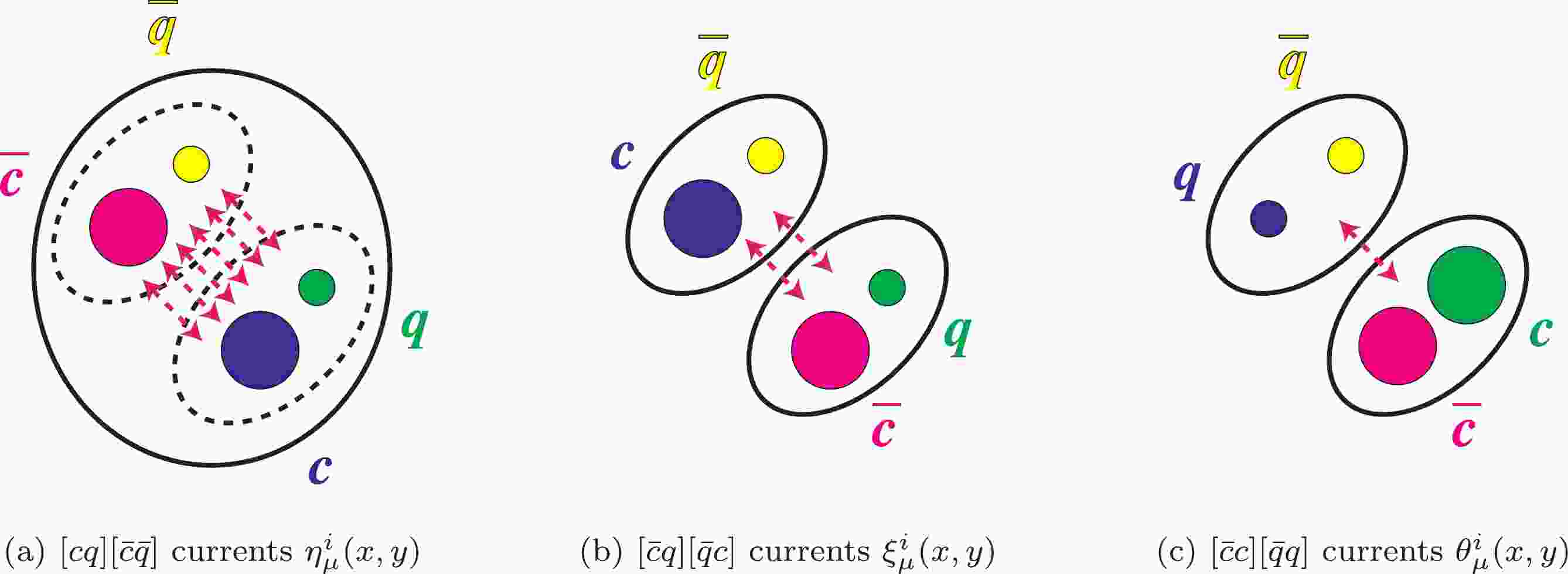
By using the c, $ \bar c $, q, $ \bar q $ quarks ($ q = u/d $), one can construct three types of tetraquark currents, as illustrated in Fig. 1: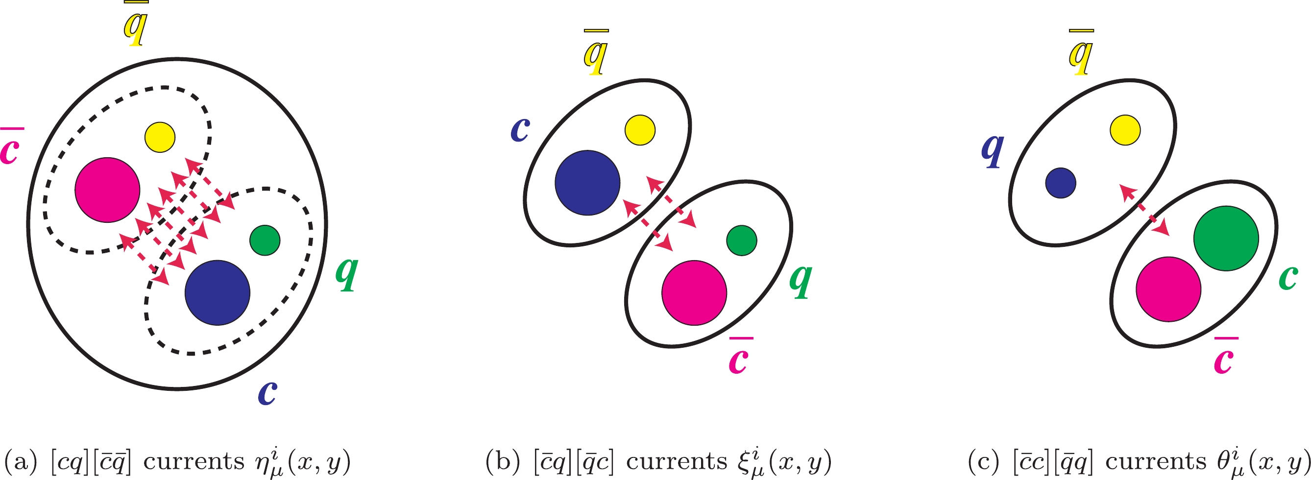

Figure 1.  (color online) Three types of tetraquark currents. Quarks are shown in red/green/blue color, and antiquarks are shown in cyan/magenta/yellow color.

where $ \Gamma_i $ are the Dirac matrices, $ {\mathbb{C}} $ is the charge-conjugation matrix, the subscripts $ a, b, c, d $ are color indices, and the sum over repeated indices is taken. One typically calls $ \eta(x,y) $ the diquark-antidiquark current, and $ \xi(x,y) $ and $ \theta(x,y) $ the mesonic-mesonic currents. We separately construct them as follows:

There are altogether eight independent $ [qc][\bar q \bar c] $ currents of $ J^{PC} = 1^{+-} $ [55]:

Here, we have omitted the coordinates x and y for simplicity. Their combinations, $ \eta^1_{\mu} - \eta^2_{\mu} $, $ \eta^3_{\mu} - \eta^4_{\mu} $, $ \eta^5_{\mu} - \eta^6_{\mu} $, and $ \eta^7_{\mu} - \eta^8_{\mu} $ have the antisymmetric color structure $ [q c]_{{\bar{\bf 3}}_c}[\bar q \bar c]_{{\bf{3}}_c}\rightarrow[c \bar c q \bar q]_{{\bf{1}}_c} $, and $ \eta^1_{\mu} + \eta^2_{\mu} $, $ \eta^3_{\mu} + \eta^4_{\mu} $, $ \eta^5_{\mu} + \eta^6_{\mu} $, and $ \eta^7_{\mu} + \eta^8_{\mu} $ have the symmetric color structure $ [q c]_{{\bf{6}}_c}[\bar q \bar c]_{{\bar{\bf 6}}_c}\rightarrow[c \bar c q \bar q]_{{\bf{1}}_c} $.

In the "type-II" diquark-antidiquark model proposed in Ref. [6], the ground-state tetraquarks can be written in the spin basis as $ |s_{qc}, s_{\bar q \bar c} \rangle_J $, where $ s_{qc} $ and $ s_{\bar q \bar c} $ are the charmed diquark and antidiquark spins, respectively. There are two ground-state diquarks: the "good" one of $ J^P = 0^+ $ and the "bad" one of $ J^P = 1^+ $ [69]. By combining them, the $ Z_c(3900) $ was interpreted as a diquark-antidiquark state of $ J^{PC} = 1^{+-} $ in Ref. [6]:

The interpolating current having the identical internal structure is simply the current $ \eta^{{\cal{Z}}}_{\mu} $ given in Eq. (2), which has been studied in Refs. [30–32, 70] using QCD sum rules:

Here, we have explicitly chosen the quark content $ [uc][\bar d \bar c] $ for the positive-charged $ Z_c(3900)^+ $.

There are altogether eight independent $ [\bar c q][\bar q c] $ currents of $ J^{PC} = 1^{+-} $:

Among them, $ \xi^{1,2,3,4}_{\mu} $ have the color structure $ [\bar c q]_{{\bf{1}}_c}[\bar q c]_{{\bf{1}}_c}\rightarrow[c \bar c q \bar q]_{{\bf{1}}_c} $, and $ \xi^{5,6,7,8}_{\mu} $ have the color structure $ [\bar c q]_{{\bf{8}}_c}[\bar q c]_{{\bf{8}}_c}\rightarrow[c \bar c q \bar q]_{{\bf{1}}_c} $. In the molecular picture, the $ Z_c(3900) $ can be interpreted as the $ D \bar D^* $ hadronic molecular state of $ J^{PC} = 1^{+-} $ [7–10]:

and the relevant interpolating current is [71–73]:

Again, we have chosen the quark content $ [\bar c u][\bar d c] $.

There are altogether eight independent $ [\bar c c][\bar q q] $ currents of $ J^{PC} = 1^{+-} $:

Among them, $ \theta^{1,2,3,4}_{\mu} $ have the color structure $ [\bar c c]_{{\bf{1}}_c}[\bar q q]_{{\bf{1}}_c}\rightarrow[c \bar c q \bar q]_{{\bf{1}}_c} $, and $ \theta^{5,6,7,8}_{\mu} $ have the color structure $ [\bar c c]_{{\bf{8}}_c}[\bar q q]_{{\bf{8}}_c}\rightarrow[c \bar c q \bar q]_{{\bf{1}}_c} $. We will discuss their corresponding hadron states in Sec. 3.

Fierz rearrangement

We have applied the Fierz rearrangement of the Dirac and color indices to systematically study light baryon and tetraquark operators/currents in Refs. [41-54]. It can also be used to relate the above three types of tetraquark currents. To do this, we must use a) the Fierz transformation [74] in the Lorentz space to rearrange the Dirac indices, and b) the color rearrangement in the color space to rearrange the color indices. All the necessary equations can be found in Sec. 3.3.2 of Ref. [75].

In Eq. (5) the Fierz rearrangement is applied to local operators/currents. However, the Fierz rearrangement is actually a matrix identity, which is valid if the same quark field in the initial and final operators is at the same location. As an example, we can apply the Fierz rearrangement to transform the non-local current with the quark fields $ \eta(x,x^{\prime};y,y^{\prime}) = [q(x) c(x^{\prime})] [\bar q(y) \bar c(y^{\prime})] $ into a combination of several non-local currents with the quark fields at the same locations $ \xi(y^{\prime},x;y,x^{\prime}) = [\bar c(y^{\prime}) q(x)] $$ [\bar q(y) c(x^{\prime})] $.

Altogether, we obtain the following relation between the currents $ \eta^i_{\mu}(x,x^{\prime};y,y^{\prime}) $ and $ \theta^i_{\mu}(y^{\prime},x^{\prime};y,x) $:

the following relation between $ \eta^i_{\mu}(x,x^{\prime};y,y^{\prime}) $ and $ \xi^i_{\mu}(y^{\prime},x;y,x^{\prime}) $:

the following relation among $ \eta^i_{\mu}(x,x^{\prime};y,y^{\prime}) $, $ \xi^{1,2,3,4}_{\mu}(y^{\prime},x;y,x^{\prime}) $, and $ \theta^{1,2,3,4}_{\mu}(y^{\prime},x^{\prime};y,x) $:

and the following relation between $ \xi^i_{\mu}(y^{\prime},x;y,x^{\prime}) $ and $ \theta^i_{\mu}(y^{\prime},x^{\prime};y,x) $:

There are altogether six types of meson operators: $ \bar q_a q_a $, $ \bar q_a \gamma_5 q_a $, $ \bar q_a \gamma_{\mu} q_a $, $ \bar q_a \gamma_{\mu} \gamma_5 q_a $, $ \bar q_a \sigma_{\mu\nu} q_a $, and $ \bar q_a \sigma_{\mu\nu} \gamma_5 q_a $. The last two can be related to each other through

The couplings of these operators to meson states are already well understood, i.e., some of them have been measured in particle experiments, and some of them have been studied and calculated by various theoretical methods, such as Lattice QCD and QCD sum rules, etc.

In this study, we require the following couplings, as summarized in Table 2:

1. The scalar operators $ J^{S} = \bar q_a q_a $ and $ I^{S} = \bar c_a c_a $ of $ J^{PC} = 0^{++} $ couple to scalar mesons. In Ref. [76] the authors used the method of QCD sum rules and extracted the coupling of $ I^{S} $ to $ \chi_{c0}(1P) $ to be

where

See also discussions in Refs. [77-79]. The light scalar mesons have a complicated nature [80], so we shall not investigate their relevant decay channels in this study.

2. The pseudoscalar operators $J^{P} = \bar q_a {\rm i}\gamma_5 q_a$ and $I^{P} = \bar c_a {\rm i}\gamma_5 c_a$ of $ J^{PC} = 0^{-+} $ couple to the pseudoscalar mesons $ \pi $ and $ \eta_c $, respectively. We can evaluate them through [81]:

3. The vector operators $ J^{V}_{\mu} = \bar q_a \gamma_{\mu} q_a $ and $ I^{V}_{\mu} = \bar c_a \gamma_{\mu} c_a $ of $ J^{PC} = 1^{–} $ couple to the vector mesons $ \rho $ and $ J/\psi $, respectively. In Refs. [82, 83] the authors used the method of Lattice QCD to obtain

where

See also discussions in Refs. [84-86].

4. The axialvector operators $ J^{A}_{\mu} = \bar q_a \gamma_{\mu} \gamma_5 q_a $ and $ I^{A}_{\mu} = \bar c_a \gamma_{\mu} \gamma_5 c_a $ of $ J^{PC} = 1^{++} $ couple to both the pseudoscalar mesons ($ \pi $ and $ \eta_c $ of $ J^{PC} = 0^{-+} $) and axialvector mesons ($ a_1(1260) $ and $ \chi_{c1}(1P) $ of $ J^{PC} = 1^{++} $). The coupling of $ J^{A}_{\mu} $ to $ \pi $ has been well measured in particle experiments [1]:

while its coupling to $ a_1(1260) $ was evaluated by using Lattice QCD [87]:

where

The coupling of $ I^{A}_{\mu} $ to $ \eta_c $ and $ \chi_{c1}(1P) $ was evaluated by using Lattice QCD [83] and QCD sum rules [77]:

where

See also discussions in Refs. [77, 85, 88-94].

5. The tensor operators $ J^{T}_{\mu\nu} = \bar q_a \sigma_{\mu\nu} q_a $ and $ I^{T}_{\mu\nu} = \bar c_a \sigma_{\mu\nu} c_a $ of $ J^{PC} = 1^{\pm-} $ couple to both the vector mesons ($ \rho $ and $ J/\psi $ of $ J^{PC} = 1^{–} $) and the axialvector mesons ($ b_1(1235) $ and $ h_{c}(1P) $ of $ J^{PC} = 1^{+-} $). The coupling of $ J^{T}_{\mu\nu} $ to $ \rho $ and $ b_1(1235) $ was calculated through Lattice QCD [82] and QCD sum rules [95]:

where

The coupling of $ I^{T}_{\mu\nu} $ to $ J/\psi $ and $ h_{c}(1P) $ was calculated through Lattice QCD [83]:

where

See also discussions in Refs. [96-104].

6. The $ Z_c(3900) $ is above the $ D \bar D^* $ threshold; thus, we need the couplings of $O^{P} = \bar q_a {\rm i}\gamma_5 c_a$ and $ O^{A}_{\mu} = \bar c_a \gamma_{\mu} \gamma_5 q_a $ to the D meson [1]:

and the couplings of $ O^{V}_{\mu} = \bar c_a \gamma_{\mu} q_a $ and $ O^{T}_{\mu\nu} = \bar q_a \sigma_{\mu\nu} c_a $ to the $ D^* $ meson [105]:

where

We found no theoretical study on the transverse decay constant $ f^T_{D^*} $; thus, we simply fit it among the decay constants, $ f_{\pi^+} $-$ f_{\rho^+} $-$ f_{\rho}^T $, $ f_{\eta_c} $-$ f_{J/\psi} $-$ f_{J/\psi}^T $, and $ f_{D} $-$ f_{D^*} $-$ f_{D^*}^T $, to obtain

See also discussions in Refs. [106, 107].

7. The $ Z_c(3900) \rightarrow D \bar D^*_0 \rightarrow D \bar D \pi $ decay is kinematically allowed, so we need the coupling of $ O^{S} = \bar q_a c_a $ to the $ D_0^* $ meson [108]:

where

See also discussions in Refs. [109, 110].

In this section and the next, we use Eqs. (16-19) derived in Sec. 2 to extract some decay properties of the $ Z_c(3900) $. The two possible interpretations of the $ Z_c(3900) $ are: a) the compact tetraquark state of $ J^{PC} = 1^{+-} $ composed of a $ J^P = 0^+ $ diquark/antidiquark and a $ J^P = 1^+ $ antidiquark/diquark [5, 6], i.e., $ |0_{qc}1_{\bar q \bar c} ; 1^{+-} \rangle $ defined in Eq. (10); and b) the $ D \bar D^* $ hadronic molecular state of $ J^{PC} = 1^{+-} $ [7–10], i.e., $ | D \bar D^*; 1^{+-} \rangle $ defined in Eq. (13). Moreover, we shall study their mixing with the $ |1_{qc}1_{\bar q \bar c} ; 1^{+-} \rangle $ and $ | D^* \bar D^*; 1^{+-} \rangle $ states, whose definitions will be given below.

In this section, we investigate the former compact tetraquark interpretation, whose relevant current $ \eta^{{\cal{Z}}}_{\mu}(x,y) $ has been given in Eq. (11). This current can be transformed to $ \theta_{\mu}^i(x,y) $ and $ \xi_{\mu}^i(x,y) $ according to Eqs. (16-18), through which we shall extract some decay properties of the $ Z_c(3900) $ as a compact tetraquark state in the following subsections.

As depicted in Fig. 2, when the c and $ \bar c $ quarks meet each other and the u and $ \bar d $ quarks meet each other at the same time, a compact tetraquark state can decay into one charmonium meson and one light meson:

Figure 2.  (color online) The decay of a compact tetraquark (diquark-antidiquark) state into one charmonium meson and one light meson. This decay can happen through either (b) a direct fall-apart process, or (c) a process with gluon(s) exchanged, that is the $ {\cal{O}}(\alpha_s)$ corrections.

The first process is a dynamical process, during which we assume that all the flavor, color, spin and orbital structures remain unchanged, so the relevant current also remains the same. The second process for $ |0_{qc}1_{\bar q \bar c} ; 1^{+-} \rangle $ can be described by transformation (16):

where we have only kept the direct fall-apart process described by $ \theta_{\mu}^{1,2,3,4} $, but neglected the $ {\cal{O}}(\alpha_s) $ corrections described by $ \theta_{\mu}^{5,6,7,8} $.

Together with Table 2, we extract the following decay channels from the above transformation:

1. The decay of $ |0_{qc}1_{\bar q \bar c} ; 1^{+-} \rangle $ into $ \eta_c\rho $ is contributed by both $ I^{P} \times J^{V}_{\mu} $ and $ I^{A,\nu} \times J^{T}_{\mu\nu} $:

where $ c_1 $ is an overall factor, related to the coupling of $ \eta^{{\cal{Z}}}_{\mu}(x,y) $ to the $ Z_c(3900)^+ $ as well as the dynamical process $ (x,y) \Longrightarrow (x^{\prime}, y^{\prime}) $ shown in Fig. 2. The two coupling constants $ g^S_{\eta_c \rho} $ and $ g^D_{\eta_c \rho} $ are defined for the S- and D-wave $ Z_c(3900) \to \eta_c \rho $ decays:

2. The decay of $ |0_{qc}1_{\bar q \bar c} ; 1^{+-} \rangle $ into $ J/\psi \pi $ is contributed by both $ I^{V}_{\mu} \times J^{P} $ and $ I^{T}_{\mu\nu} \times J^{A,\nu} $:

The two coupling constants $ g^S_{\psi \pi} $ and $ g^D_{\psi \pi} $ are defined for the S- and D-wave $ Z_c(3900) \rightarrow J/\psi \pi $ decays respectively:

3. The decay of $ |0_{qc}1_{\bar q \bar c} ; 1^{+-} \rangle $ into $ \eta_c b_1 $ is contributed by $ I^{A,\nu} \times J^{T}_{\mu\nu} $:

This process is kinematically forbidden, but the $ |0_{qc}1_{\bar q \bar c} ; 1^{+-} \rangle \rightarrow \eta_c b_1 \rightarrow \eta_c \omega \pi \rightarrow \eta_c + 4 \pi $ decay is kinematically allowed.

4. The decay of $ |0_{qc}1_{\bar q \bar c} ; 1^{+-} \rangle $ into $ \chi_{c1} \rho $ is contributed by $ I^{A,\nu} \times J^{T}_{\mu\nu} $:

This process is kinematically forbidden, but the $ |0_{qc}1_{\bar q \bar c} ; 1^{+-} \rangle \rightarrow \chi_{c1} \rho \rightarrow \chi_{c1} \pi \pi $ decay is kinematically allowed.

5. The decay of $ |0_{qc}1_{\bar q \bar c} ; 1^{+-} \rangle $ into $ \chi_{c1} b_1 $ is contributed by $ I^{A,\nu} \times J^{T}_{\mu\nu} $:

This process is kinematically forbidden.

6. The decay of $ |0_{qc}1_{\bar q \bar c} ; 1^{+-} \rangle $ into $ h_c \pi $ is contributed by $ I^{T}_{\mu\nu} \times J^{A,\nu} $:

This process is kinematically allowed.

7. The decay of $ |0_{qc}1_{\bar q \bar c} ; 1^{+-} \rangle $ into $ J/\psi a_1 $ is contributed by $ I^{T}_{\mu\nu} \times J^{A,\nu} $:

This process is kinematically forbidden, but the $ |0_{qc}1_{\bar q \bar c} ; 1^{+-} \rangle \rightarrow J/\psi a_1 \rightarrow J/\psi \rho \pi \rightarrow J/\psi + 3 \pi $ decay is kinematically allowed.

8. The decay of $ |0_{qc}1_{\bar q \bar c} ; 1^{+-} \rangle $ into $ h_c a_1 $ is contributed by $ I^{T}_{\mu\nu} \times J^{A,\nu} $:

This process is kinematically forbidden.

Summarizing the above results, we numerically obtain

From these coupling constants, we further obtain the following relative branching ratios, which are kinematically allowed:

In addition, the following decay chains are also possible but have quite small partial decay widths:

As depicted in Fig. 3, when the c and $ \bar d $ quarks meet each other and the u and $ \bar c $ quarks meet each other at the same time, a compact tetraquark state can decay into two charmed mesons. This process for $ |0_{qc}1_{\bar q \bar c} ; 1^{+-} \rangle $ can be described by transformation (17):

Figure 3.  (color online) The decay of a compact tetraquark (diquark-antidiquark) state into two charmed mesons. This decay can happen through either (b) a direct fall-apart process, or (c) a process with gluon(s) exchanged, that is the $ {\cal{O}}(\alpha_s)$ corrections.

Again, we have only kept the direct fall-apart process described by $ \xi_{\mu}^{2,3} $, but neglected the $ {\cal{O}}(\alpha_s) $ corrections described by $ \xi_{\mu}^{6,7} $.

The term $ \xi_{\mu}^{2} $ couples to the $ D^*\bar D^* $ and $ D^* \bar D_1 $ final states, and the term $ \xi_{\mu}^{3} $ couples to the $ D \bar D_0^* $ and $ D_1 \bar D_0^* $ final states. Among them, only the $ |0_{qc}1_{\bar q \bar c} ; 1^{+-} \rangle \rightarrow D \bar D^*_0 \rightarrow D \bar D \pi $ decay is kinematically allowed, contributed by $ \xi_{\mu}^{3} = O^{A}_{\mu} \times O^{S} $ to be:

where $ c_2 $ is an overall factor.

Thus, we numerically obtain

Comparing the $ |0_{qc}1_{\bar q \bar c} ; 1^{+-} \rangle \rightarrow D \bar D^*_0 \rightarrow D \bar D \pi $ decay studied in the present subsection with the $ |0_{qc}1_{\bar q \bar c} ; 1^{+-} \rangle \rightarrow J/\psi \pi $ and $ |0_{qc}1_{\bar q \bar c} ; 1^{+-} \rangle \rightarrow \eta_c\rho $ decays studied in the previous subsection, we obtain

The current $ \eta^{{\cal{Z}}}_{\mu}(x,y) $ does not correlate with the two terms $\xi_{\mu}^{1} = -{\rm i} O^{V}_{\mu} \times O^{P}$ and $ \xi_{\mu}^{4} = O^{A,\nu} \times O^{T}_{\mu\nu} $, both of which can couple to the $ D \bar D^* $ final state. This suggests that $ |0_{qc}1_{\bar q \bar c} ; 1^{+-} \rangle $ does not decay to the $ D \bar D^* $ final state with a large branching ratio,

so that

Eqs. (62) and (64) together suggest that $ |0_{qc}1_{\bar q \bar c} ; 1^{+-} \rangle $ mainly decays into one charmonium meson and one light meson, other than two charmed mesons.

If the above two processes investigated in Sec. 4.1 and Sec. 4.2 happen at the same time, we can use the transformation (18); i.e., $ |0_{qc}1_{\bar q \bar c} ; 1^{+-} \rangle $ can decay into one charmonium meson and one light meson as well as two charmed mesons at the same time, the process of which is described by the color-singlet-color-singlet currents $ \theta_{\mu}^{1,2,3,4} $ and $ \xi_{\mu}^{1,2,3,4} $ together:

Here, we have kept all the terms, and there is no $ \cdots $ in this equation.

Comparing the above equation with Eqs. (42) and (58), we obtain the same relative branching ratios as Sec. 4.1 and Sec. 4.2, with just the overall factors $ c_1 $ and $ c_2 $ replaced by others.

The relative branching ratio $ {\cal{R}}_{Z_c} $ calculated in Sec. 4.1 is only $ 0.059 $, which is significantly smaller than the BESIII measurement $ {\cal{R}}_{Z_c} = 2.2 \pm 0.9 $ at $ \sqrt{s} = 4.226 $ GeV [29]. In this subsection we slightly modify the internal structure of the $ Z_c(3900) $ to reevaluate this ratio.

Actually, in the Type-II diquark-antidiquark model [6], the $ Z_c(3900) $ was interpreted as

and the ratio $ {\cal{R}}_{Z_c} $ was predicted to be $ 0.27^{+0.40}_{-0.17} $ [40]; while in the Type-I diquark-antidiquark model [5], the $ Z_c(3900) $ was interpreted as the mixing state

where

and a small $ |1_{qc}1_{\bar q \bar c} ; 1^{+-} \rangle $ component is able to increase this ratio to $ \left( 2.3^{+3.3}_{-1.4} \right) \times 10^2 $ [40], which is almost one thousand times larger.

Thus, we attempt to add this $ |1_{qc}1_{\bar q \bar c} ; 1^{+-} \rangle $ component in this subsection. The interpolating current having the identical internal structure is

so that $ |x_{qc}1_{\bar q \bar c} ; 1^{+-} \rangle $ can be described by

which transforms according to Eq. (16) as:

Note that the two mixing angles $ \theta_1 $ and $ \theta^{\prime}_1 $ are not necessarily the same (and probably not the same), but they can be related to each other, i.e.,

To solve this relation, we must determine the couplings of $ \eta^{{\cal{Z}}}_{\mu} $ and $ \eta^{{\cal{Z}}^{\prime}}_{\mu} $ to $ |0_{qc}1_{\bar q \bar c} ; 1^{+-} \rangle $ and $ |1_{qc}1_{\bar q \bar c} ; 1^{+-} \rangle $, which we shall not investigate in this study. Nonetheless, we can plot the three ratios

as functions of the mixing angle $ \theta^{\prime}_1 $, as shown in Fig. 4. We find that $ {\cal{R}}_{\psi \pi} $ decreases and $ {\cal{R}}_{\eta_c \rho} $ increases, so that the ratio $ {\cal{R}} $ increases rapidly as the mixing angle $ \theta^{\prime}_1 $ decreases from $ 0 $ to $ -10^{\rm{o}} $.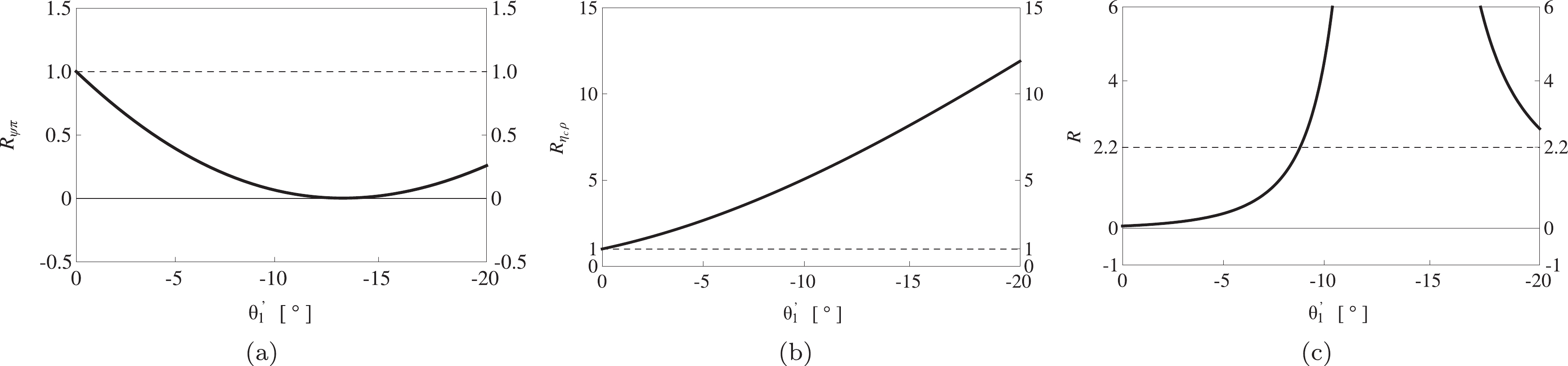

Figure 4.  The ratios (a) $ {\cal{R}}_{\psi\pi} \equiv \dfrac{\Gamma(|x_{qc}1_{\bar q \bar c} ; 1^{+-} \rangle \rightarrow J/\psi\pi) }{ \Gamma(|0_{qc}1_{\bar q \bar c}; 1^{+-} \rangle \rightarrow J/\psi\pi)} $, (b) $ {\cal{R}}_{\eta_c\rho} \equiv \dfrac{\Gamma(|x_{qc}1_{\bar q \bar c} ; 1^{+-} \rangle \rightarrow \eta_c\rho) }{ \Gamma(|0_{qc}1_{\bar q \bar c}; 1^{+-} \rangle \rightarrow \eta_c\rho)} $, and (c) $ {\cal{R}} \equiv \dfrac{{\cal{B}}(|x_{qc}1_{\bar q \bar c} ; 1^{+-} \rangle \rightarrow \eta_c\rho) }{{\cal{B}}(|x_{qc}1_{\bar q \bar c} ; 1^{+-} \rangle \rightarrow J/\psi\pi)} $ as functions of the mixing angle $ \theta^{\prime}_1 $.

Especially, after fine-tuning $ \theta^{\prime}_1 = -8.8^{\rm{o}} $, we obtain

The first ratio $ {\cal{R}} $ is 2.2, which is the same as the BESIII measurement $ {\cal{R}}_{Z_c} = 2.2 \pm 0.9 $ [29].

The decay of $ |x_{qc}1_{\bar q \bar c} ; 1^{+-} \rangle $ into two charmed mesons can be described by the current $ \eta^{\rm{mix}}_{\mu}(x,y) $ together with the transformation (17):

so that

Hence, $ |x_{qc}1_{\bar q \bar c} ; 1^{+-} \rangle $ can decay into the $ D \bar D^* $ final state, which is consistent with the BESIII observations [26, 27]. Moreover, it was proposed in Ref. [67] that to enable the decay of the $ Z_c(3900) $, a constituent of a diquark must tunnel through the barrier of the diquark-antidiquark potential. However, this tunnelling for heavy quarks is exponentially suppressed compared to that for light quarks, so the compact tetraquark couplings are expected to favour the open charm modes with respect to charmonium ones. Thus, $ c_2 $ may be significantly larger than $ c_1 $, so that $ |x_{qc}1_{\bar q \bar c} ; 1^{+-} \rangle $ may mainly decay into two charmed mesons.

Another possible interpretation of the $ Z_c(3900) $ is the $ D \bar D^* $ hadronic molecular state of $ J^{PC} = 1^{+-} $ [7–10], i.e., $ | D \bar D^*; 1^{+-} \rangle $ defined in Eq. (13). Its relevant current $ \xi^{{\cal{Z}}}_{\mu}(x,y) $ has been given in Eq. (14). We can transform this current to $ \theta_{\mu}^i(x,y) $ according to transformation (19), through which we shall extract some decay properties of the $ Z_c(3900) $ as a hadronic molecular state in the following subsections.

As depicted in Fig. 5, when the c and $ \bar c $ quarks meet each other and the u and $ \bar d $ quarks meet each other at the same time, a hadronic molecular state can decay into one charmonium meson and one light meson. This process for $ | D \bar D^*; 1^{+-} \rangle $ can be described by transformation (19):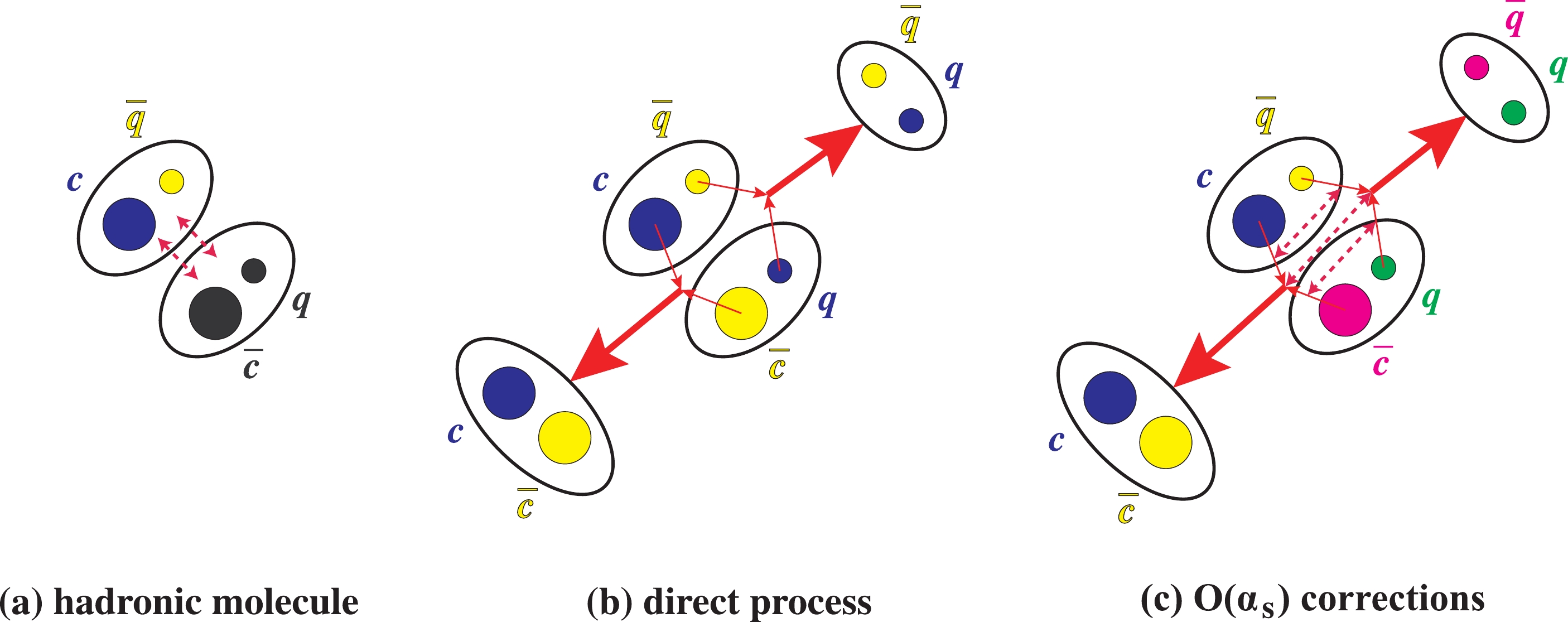

Figure 5.  (color online) The decay of a hadronic molecular state into one charmonium meson and one light meson. This decay can happen through either (b) a direct fall-apart process, or (c) a process with gluon(s) exchanged, that is the $ {\cal{O}}(\alpha_s)$ corrections.

where we have only kept the direct fall-apart process described by $ \theta_{\mu}^{1,2,3,4} $, but neglected the $ {\cal{O}}(\alpha_s) $ corrections described by $ \theta_{\mu}^{5,6,7,8} $.

We repeat the same procedures as those performed in Sec. 4.1, and extract the following coupling constants from this transformation:

The above coupling constants are related to the S- and D-wave $ | D \bar D^*; 1^{+-} \rangle \to \eta_c \rho $ decays, the S- and D-wave $ | D \bar D^*; 1^{+-} \rangle \rightarrow J/\psi \pi $ decays, and the $ | D \bar D^*; 1^{+-} \rangle \rightarrow \eta_c b_1 $, $ \chi_{c1} \rho $, $ \chi_{c1} b_1 $, $ h_c \pi $, $ J/\psi a_1 $, $ h_c a_1 $ decays, respectively. All of them contain an overall factor of $ c_4 $.

Using the above coupling constants, we further obtain

These values are surprisingly the same as Eqs. (56), obtained in Sec. 4.1 for the compact tetraquark state $ |0_{qc}1_{\bar q \bar c} ; 1^{+-} \rangle $.

Assuming the $ Z_c(3900) $ to be the $ D \bar D^* $ hadronic molecular state of $ J^{PC} = 1^{+-} $, it can naturally decay to the $ D \bar D^* $ final state, of which the fall-apart process can be described by

The decay of $ | D \bar D^*; 1^{+-} \rangle $ into the $ D \bar D^{*} $ final state is contributed by this term to be

where $ c_5 $ is an overall factor, and is likely larger than $ c_4 $. Numerically, we obtain

Comparing the $ | D \bar D^*; 1^{+-} \rangle \rightarrow D \bar D^{*} $ decay studied in the present subsection with the $ | D \bar D^*; 1^{+-} \rangle \rightarrow J/\psi \pi $ and $ | D \bar D^*; 1^{+-} \rangle \rightarrow \eta_c\rho $ decays studied in the previous subsection, we obtain

The current $ \xi^{{\cal{Z}}}_{\mu}(x,y) $ does not correlate with the term $ \xi_{\mu}^{3} = O^{A}_{\mu} \times O^{S} $, so that $ | D \bar D^*; 1^{+-} \rangle $ does not decay into the $ D \bar D_0^{*} $ final state

Eqs. (83) and (84) suggest that $ | D \bar D^*; 1^{+-} \rangle $ mainly decays into two charmed mesons, other than one charmonium meson and one light meson. This conclusion is opposite to the one obtained in Sec. 4.2 for the compact tetraquark state $ |0_{qc}1_{\bar q \bar c} ; 1^{+-} \rangle $.

Similarly to Sec. 4.4, we add a small $ | D^* \bar D^*; 1^{+-} \rangle $ component

to $ | D \bar D^*; 1^{+-} \rangle $ in this subsection to reevaluate the ratio $ {\cal{R}}_{Z_c} $. The interpolating current having the same internal structure as $ | D^* \bar D^*; 1^{+-} \rangle $ is

so that we can use

to described the mixed molecular state

The current $ \xi^{\rm{mix}}_{\mu}(x,y) $ transforms according to Eq. (19) to be

After fine-tuning $ \theta^{\prime}_2 = -8.8^{\rm{o}} $, we obtain

the values of which are the same as those in Eqs. (78) obtained in Sec. 4.1 for the mixed compact tetraquark state $ |x_{qc}1_{\bar q \bar c} ; 1^{+-} \rangle $. In fact, we can also plot the following three ratios

as functions of the mixing angle $ \theta^{\prime}_2 $, and the obtained figures are identical to Fig. 4, where $ {\cal{R}}_{\psi \pi} $, $ {\cal{R}}_{\eta_c \rho} $, and $ {\cal{R}} $ are shown as functions of $ \theta^{\prime}_1 $.

We also obtain

suggesting that $ |D^{(*)} \bar D^*; 1^{+-} \rangle $ mainly decays into two charmed mesons.

In this paper we systematically construct all the tetraquark currents/operators of $ J^{PC} = 1^{+-} $ with the quark content $ c \bar c q \bar q $ ($ q = u/d $). There are three configurations: $ [cq][\bar c \bar q] $, $ [\bar c q][\bar q c] $, and $ [\bar c c][\bar q q] $, and for each configuration we construct eight independent currents. We use the Fierz rearrangement of the Dirac and color indices to derive their relations, through which we study the strong decay properties of the $ Z_c(3900) $:

● Using the transformation of $ [qc][\bar q \bar c] \to [\bar c c][\bar q q] $, we study the decay properties of the $ Z_c(3900) $ as a compact diquark-antidiquark tetraquark state into one charmonium meson and one light meson.

● Using the transformation of $ [qc][\bar q \bar c] \to [\bar c q][\bar q c] $, we study the decay properties of the $ Z_c(3900) $ as a compact diquark-antidiquark tetraquark state into two charmed mesons.

● We use the transformation of the $ [qc][\bar q \bar c] $ currents to the color-singlet-color-singlet $ [\bar c c][\bar q q] $ and $ [\bar c q][\bar q c] $ currents, and obtain the same relative branching ratios as the above results.

● Using the transformation of $ [\bar c q][\bar q c] \to [\bar c c][\bar q q] $, we study the decay properties of the $ Z_c(3900) $ as a hadronic molecular state into one charmonium meson and one light meson.

● Through the $ [\bar c q][\bar q c] $ currents themselves, we study the decay properties of the $ Z_c(3900) $ as a hadronic molecular state into two charmed mesons.

Our results suggest that the possible decay channels of the $ Z_c(3900) $ are: a) the two-body decays $ Z_c(3900) \to J/\psi\pi $, $ Z_c(3900) \to \eta_c\rho $, $ Z_c(3900) \to h_c\pi $, and $ Z_c(3900) \to D \bar D^{*} $, b) the three-body decays $ Z_c(3900) \rightarrow $$\chi_{c1}\rho \rightarrow \chi_{c1}\pi \pi $ and $ Z_c(3900) \rightarrow D \bar D_0^{*} + \bar D D_0^{*} \rightarrow D \bar D \pi $, and c) the many-body decay chains $ Z_c(3900) \rightarrow J/\psi a_1 \rightarrow J/\psi \rho \pi $$ \rightarrow J/\psi + 3 \pi $ and $ Z_c(3900) \rightarrow \eta_c b_1 \rightarrow \eta_c \omega \pi \rightarrow \eta_c + 4 \pi $. Their relative branching ratios are summarized in Table 3, where we have investigated the following interpretations of the $ Z_c(3900) $:

channels	$|0_{qc}1_{\bar q \bar c}; 1^{+-} \rangle$	$|x_{qc}1_{\bar q \bar c} ; 1^{+-} \rangle$($\theta^{\prime}_1 = -8.8^{\rm{o}}$)	$|D \bar D^*; 1^{+-} \rangle$	$|D^{(*)} \bar D^*; 1^{+-} \rangle$($\theta^{\prime}_2 = -8.8^{\rm{o}}$)
$\dfrac {{\cal{B}}(Z_c \rightarrow \eta_c\rho)}{ {\cal{B}}(Z_c \rightarrow J/\psi\pi)}}$	$0.059$	$2.2$ (input)	$0.059$	$2.2$ (input)
$ {{\cal{B}}(Z_c \rightarrow h_c\pi)}{ {\cal{B}}(Z_c \rightarrow J/\psi\pi)}$	$0.0088$	$0.052$	$0.0088$	$0.052$
$\dfrac {{\cal{B}}(Z_c \rightarrow \chi_{c1}\rho \rightarrow \chi_{c1} \pi \pi) }{{\cal{B}}(Z_c \rightarrow J/\psi\pi)}}$	$1.4 \times 10^{-6}$	$1.5 \times 10^{-5}$	$1.4 \times 10^{-6}$	$1.5 \times 10^{-5}$
$\dfrac {{\cal{B}}(Z_c \rightarrow D \bar D^{*} + \bar D D^{*})}{{\cal{B}}(Z_c \rightarrow J/\psi\pi + \eta_c\rho)}}$	$\approx 0$	$0.26 t_1$	$25 t_2$	$67 t_2$
$\dfrac {{\cal{B}}(Z_c \rightarrow D \bar D_0^{*} + \bar D D_0^{*} \rightarrow D \bar D \pi)} {{\cal{B}}(Z_c \rightarrow J/\psi\pi + \eta_c\rho)}}$	$9.3 t_1 \times 10^{-8}$	$2.5 t_1 \times 10^{-7}$	$\approx 0$	$\approx 0$

Table 3.  Relative branching ratios of the $Z_c(3900)$ evaluated through the Fierz rearrangement. $\theta_{1,2}^{\prime}$ are the two mixing angles defined in Eqs. (69) and (87), which are fine-tuned to be $\theta^{\prime}_1 = \theta^{\prime}_2 = -8.8^{\rm{o}}$, so that $\dfrac{{\cal{B}}(|x_{qc}1_{\bar q \bar c} ; 1^{+-} \rangle \rightarrow \eta_c\rho) }{ {\cal{B}}(|x_{qc}1_{\bar q \bar c} ; 1^{+-} \rangle \rightarrow J/\psi\pi)} = \dfrac{{\cal{B}}(|D^{(*)} \bar D^*; 1^{+-} \rangle \rightarrow \eta_c\rho)}{ {\cal{B}}(|D^{(*)} \bar D^*; 1^{+-} \rangle \rightarrow J/\psi\pi)} = 2.2$ [29]. In this table, we do not take into account the phase angle $\phi$ between S- and D-wave coupling constants.

● In the second and third columns of Table 3, $ |0_{qc}1_{\bar q \bar c} ; 1^{+-} \rangle $ and $ |x_{qc}1_{\bar q \bar c} ; 1^{+-} \rangle $ denote the compact tetraquark states of $ J^{PC} = 1^{+-} $, as defined in Eq. (10) and Eq. (66), respectively. In particular, we have considered the mixing between the compact tetraquarks states

Using the mixing angle $ \theta^{\prime}_1 = -8.8^{\rm{o}} $, we obtain

● In the fourth and fifth columns of Table 3, $ | D \bar D^*; 1^{+-} \rangle $ and $ |D^{(*)} \bar D^*; 1^{+-} \rangle $ denote the hadronic molecular states of $ J^{PC} = 1^{+-} $, defined in Eq. (13) and Eq. (88), respectively. Especially, we have considered the mixing between the hadronic molecule states

Using the mixing angle $ \theta^{\prime}_2 = -8.8^{\rm{o}} $, we obtain

In the above expressions, we have used the recent BESIII measurement $ {\cal{R}}_{Z_c} \equiv \dfrac{{\cal{B}}(Z_c(3900) \rightarrow \eta_c\rho) }{ {\cal{B}}(Z_c(3900) \rightarrow J/\psi\pi)} = 2.2 \pm 0.9 $ [29] as an input to determine the mixing angles $ \theta^{\prime}_1 $ and $ \theta^{\prime}_2 $. The ratio $ t_1 \equiv {c_2^2 / c_1^2} $ is the parameter measuring which process happens more easily, the process depicted in Fig. 2(b) or the process depicted in Fig. 3(b). Generally, the exchange of one light quark with another light quark seems to be easier than the exchange of one light quark with another heavy quark [67, 111]. Thus, it can be the case that $ t_1 \geq 1 $. As discussed in Sec. 5.2, $ c_5 $ is likely larger than $ c_4 $, so that the other ratio $ t_2 \equiv {c_5^2 / c_4^2} \geq 1 $.

The above relative branching ratios calculated in the present study turn out to be very different, which may be one of the reasons why many multiquark states were observed in only a few decay channels [75]. Note that in order to extract the above results, we have only considered the leading-order fall-apart decays described by color-singlet-color-singlet meson-meson currents but neglected the $ {\cal{O}}(\alpha_s) $ corrections described by color-octet-color-octet meson-meson currents. This means that there can be other decay channels.

Based on Table 3 as well as Eqs. (94) and (96), we conclude this paper:

● The relative branching ratios $ \dfrac{{\cal{B}}(|0_{qc}1_{\bar q \bar c} ; 1^{+-} \rangle \rightarrow \eta_c\rho) }{ {\cal{B}}(|0_{qc}1_{\bar q \bar c} ; 1^{+-} \rangle \rightarrow J/\psi\pi)} $ and $ \dfrac{{\cal{B}}(| D \bar D^*; 1^{+-} \rangle \rightarrow \eta_c\rho) }{{\cal{B}}(| D \bar D^*; 1^{+-} \rangle \rightarrow J/\psi\pi)} $ are both around 0.059, significantly smaller than the BESIII measurement $ {\cal{R}}_{Z_c} = 2.2 \pm 0.9 $ at $ \sqrt{s} = 4.226 $ GeV [29]. However, we can add a small $ |1_{qc}1_{\bar q \bar c} ; 1^{+-} \rangle $ component to $ |0_{qc}1_{\bar q \bar c} ; 1^{+-} \rangle $ to obtain $ \dfrac{{\cal{B}}(|x_{qc}1_{\bar q \bar c} ; 1^{+-} \rangle \rightarrow \eta_c\rho) }{ {\cal{B}}(|x_{qc}1_{\bar q \bar c} ; 1^{+-} \rangle \rightarrow J/\psi\pi)} = 2.2 $; we can also add a small $ |D^{*} \bar D^*; 1^{+-} \rangle $ component to $ | D \bar D^*; 1^{+-} \rangle $ to obtain $ \dfrac{{\cal{B}}(|D^{(*)} \bar D^*; 1^{+-} \rangle \rightarrow \eta_c\rho) }{{\cal{B}}(|D^{(*)} \bar D^*; 1^{+-} \rangle \rightarrow J/\psi\pi)} = 2.2 $. Note that if the relevant mixing angles change dynamically, the ratio $ {\cal{R}}_{Z_c} $ would also change dynamically.

● The relative branching ratios of the $ | D \bar D^*; 1^{+-} \rangle $ decays into one charmonium meson and one light meson are the same as those of the $ |0_{qc}1_{\bar q \bar c} ; 1^{+-} \rangle $ decays. After taking proper mixing angles, the relative branching ratios of the $ |D^{(*)} \bar D^*; 1^{+-} \rangle $ decays into one charmonium meson and one light meson are also the same as those of the $ |x_{qc}1_{\bar q \bar c} ; 1^{+-} \rangle $ decays. This suggests that one may not discriminate between the compact tetraquark and hadronic molecule scenarios by only investigating relative branching ratios of the $ Z_c(3900) $ decays into one charmonium meson and one light meson.

● $ |0_{qc}1_{\bar q \bar c} ; 1^{+-} \rangle $ mainly decays into one charmonium meson and one light meson, but $ |x_{qc}1_{\bar q \bar c} ; 1^{+-} \rangle $ might mainly decay into two charmed mesons after taking into account the barrier of the diquark-antidiquark potential (see detailed discussions in Ref. [67] proposing $ c_2 \gg c_1 $). Both $ | D \bar D^*; 1^{+-} \rangle $ and $ |D^{(*)} \bar D^*; 1^{+-} \rangle $ mainly decay into two charmed mesons.

It is useful to generally discuss our uncertainty. In this study, we have worked within the naive factorization scheme; thus, our uncertainty is greater than that of well-developed QCD factorization method [62–64], which is at 5% when being applied to study the weak and radiative decay properties of conventional (heavy) hadrons. On the other hand, the tetraquark decay constant $ f_{Z_c} $ is removed when calculating relative branching ratios. This significantly reduces our uncertainty because this parameter has not yet been accurately determined. Hence, we estimate our uncertainty to be approximately$ X^{+100\%}_{-\; 50\%} $.

Next,let us compare our results with other theoretical calculations. First, we compare them with the QCD sum rule results obtained in Refs. [30, 31], where the $ Z_c(3900) $ is assumed to be a compact diquark-antidiquark tetraquark state. In this study, we find that decays of the $ Z_c(3900) $ into $ J/\psi\pi $ and $ \eta_c\rho $ can happen through both the S-wave and D-wave, and we have calculated these two amplitudes together, as shown in Eqs. (43-48); we can also calculate them individually and obtain

In the former equation we have only considered the S-wave amplitudes, and in the latter, only the D-wave amplitudes. The QCD sum rule study in Ref. [30] only considers the S-wave amplitudes, where they obtained

so that

The QCD sum rule study in Ref. [31] only considers the D-wave amplitudes, where they obtained

so that

Hence, our results are more or less consistent with the QCD sum rule calculations [30, 31]. Here, we would like to note that the D-wave decay amplitudes are important and cannot be neglected:

In fact, there is still one parameter not considered in our calculations: the phase angle $ \phi $ between the S- and D-wave decay amplitudes. For completeness, we shall investigate its relevant uncertainty in Appendix A.

Following this, we compare our results with Ref. [40], where the authors assumed the $ Z_c(3900) $ to be a hadronic molecular state and used the Non-Relativistic Effective Field Theory (a framework based on HQET and NRQCD) to obtain

This value is well consistent with our result

Finally, we propose the BESIII, Belle, Belle-II, and LHCb Collaborations to search for those decay channels not yet observed, in order to better understand the nature of the $ Z_c(3900) $.

We thank Fu-Sheng Yu and Qin Chang for helpful discussions.

There are two different effective Lagrangians for the $ Z_c(3900) $ decay into the $ \eta_c \rho $ final state, as given in Eqs. (44) and (45):

There are also two different effective Lagrangians for the $ Z_c(3900) $ decay into the $ J/\psi \pi $ final state, as given in Eqs. (47) and (48):

There can be a phase angle $ \phi $ between $ g^S_{\eta_c \rho} $ and $ g^D_{\eta_c \rho} $, as well as between $ g^S_{\psi \pi} $ and $ g^D_{\psi \pi} $. This parameter is unknown and therfore not fixed, because QCD sum rules dictate that one can only calculate the modular square of the decay constant, such as $ |f_{\eta_c}|^2 $. This might also be the case for Lattice QCD and the light front model. For example, see the different definitions of $ f_{\eta_c} $ in Refs. [83, 91].

We rotate this phase angle between all S- and D-wave coupling constants to be $ \phi = \pi $, and revise the previous calculations. The results are summarized in Table A1. In particular, using the mixing angle $ \theta^{\prime}_1 = \theta^{\prime}_2 = -10.1^{\rm{o}} $, we obtain

channels	$|0_{qc}1_{\bar q \bar c}; 1^{+-} \rangle$	$|x_{qc}1_{\bar q \bar c} ; 1^{+-} \rangle$($\theta^{\prime}_1 = -10.1^{\rm{o}}$)	$|D \bar D^*; 1^{+-} \rangle$	$|D^{(*)} \bar D^*; 1^{+-} \rangle$($\theta^{\prime}_2 = -10.1^{\rm{o}}$)
$\dfrac{{\cal{B}}(Z_c \rightarrow \eta_c\rho)}{ {\cal{B}}(Z_c \rightarrow J/\psi\pi)}$	$0.36$	$2.2$ (input)	$0.36$	$2.2$ (input)
$\dfrac{{\cal{B}}(Z_c \rightarrow h_c\pi) }{ {\cal{B}}(Z_c \rightarrow J/\psi\pi)}$	$0.0018$	$0.0038$	$0.0018$	$0.0038$
$\dfrac{{\cal{B}}(Z_c \rightarrow \chi_{c1}\rho \rightarrow \chi_{c1} \pi \pi) }{ {\cal{B}}(Z_c \rightarrow J/\psi\pi)}$	$2.8 \times 10^{-7}$	$1.2 \times 10^{-6}$	$2.8 \times 10^{-7}$	$1.2 \times 10^{-6}$
$\dfrac{{\cal{B}}(Z_c \rightarrow D \bar D^{*} + \bar D D^{*}) }{ {\cal{B}}(Z_c \rightarrow J/\psi\pi + \eta_c\rho)}$	$\approx 0$	$0.059 t_1$	$3.9 t_2$	$5.2 t_2$
$\dfrac{{\cal{B}}(Z_c \rightarrow D \bar D_0^{*} + \bar D D_0^{*} \rightarrow D \bar D \pi)}{ {\cal{B}}(Z_c \rightarrow J/\psi\pi + \eta_c\rho)}$	$1.5 t_1 \times 10^{-8}$	$2.0 t_1 \times 10^{-8}$	$\approx 0$	$\approx 0$

Table A1.  Relative branching ratios of the $Z_c(3900)$ evaluated through the Fierz rearrangement. The two mixing angles are fine-tuned to be $\theta^{\prime}_1 = \theta^{\prime}_2 = -10.1^{\rm{o}}$, so that $\dfrac{{\cal{B}}(|x_{qc}1_{\bar q \bar c} ; 1^{+-} \rangle \rightarrow \eta_c\rho) }{{\cal{B}}(|x_{qc}1_{\bar q \bar c} ; 1^{+-} \rangle \rightarrow J/\psi\pi)} = \dfrac{{\cal{B}}(|D^{(*)} \bar D^*; 1^{+-} \rangle \rightarrow \eta_c\rho)}{ {\cal{B}}(|D^{(*)} \bar D^*; 1^{+-} \rangle \rightarrow J/\psi\pi)} = 2.2$ [29]. In this table, we fix the phase angle $\theta$ between all the S- and D-wave coupling constants to be $\theta = \pi$.