


 Abstract
 HTML
HTML Reference
 Related
 PDF
PDF


-
The introduction of the complex angular momentum l in the potential scattering gives rise to poles representing bound states or resonances for
$ l>0 $ [1-3]. As is well-known, the application of Regge's original ideas to the high energy scattering of elementary particles results in a very successful theory. For example, the broad class of reactions that can be explained in a unified view led Donnachie and Landshoff to conjecture that the Regge theory would be part of the truth of particle physics [4]. In other words: if such formalism is wrong, then it is probably wrong due to some minor misunderstanding.The main entity in the Regge theory is the
$ \alpha(t) $ trajectory, which is a phenomenological input within the formalism. The location of a pole corresponds to a bound state, and the scattering amplitude behavior is controlled by this leading Regge pole. Then, a resonance with spin j turns necessary to include the excitation$ j+2 $ ,$ j+4 $ ,···, keeping fixed the other quantum numbers. These particles lie on the Regge trajectory, obtained from the so-called Chew-Frautschi plot [5, 6]. The Regge trajectory is assumed to be linear for light mesons and baryons [7], whose parameters can be extracted from the scattering data as well as from the particle spectra. However, an important question without an answer is if these trajectories are linear everywhere or only at the asymptotic regime. Moreover, the analyticity and unitarity properties require that$ \alpha(t) $ be a non-linear complex-valued function [8, 9].The Pomeranchuk theorem asserts that the total cross-section of the particle-particle and particle-antiparticle at high energies should tend to the same limit [10]. This theorem creates the need for the exchange of a state, with the quantum numbers of the vacuum, that does not distinguish particles from antiparticles in the asymptotic energy regime. This is the role played by the leading Regge pole, the so-called pomeron, in the particle scattering at high energies, and the reason supporting its existence is entirely phenomenological. The problem here is that
$ \alpha(t) $ for the pomeron can only be obtained from the experimental data, as it has no particle spectrum. However, if one extrapolates the pomeron trajectory from negative to positive values, then one can predict glueball states with the integer spin. The first mention to the pomeron as a pair of gluons in a color singlet is attributed to Low and Nussinov [11, 12]. Nonetheless, there is no experimental evidence for the pomeron in present-day energies.The odderon, the counterpart of the pomeron, can distinguish particles from antiparticles in the convenient energy range. The original idea of the odderon is attributed to Bouquet et al. [13] and Joynson et al. [14], and the proposition of the odderon as the exchange of three reggeized gluons is attributed to Bartels [15], followed closely by Refs. [16, 17], being a formal QCD prediction. In contrast, considering the t-dependence of the differential cross-section, the general belief is that the odderon is responsible for the pronounced dip in the proton-proton scattering. In contrast, it fills the dip in the case of the proton-antiproton differential cross-section. Differently from the pomeron, the odderon has possible experimental evidence [18], which is subject to discussions in the literature [19-21].
For a long time, the Regge theory was known to be valid in the perturbation theory. Indeed, the Regge trajectory can also be obtained from the Bethe-Salpeter equation [22]. The BFKL equation likewise results in the pomeron [23, 24]. This leading Regge pole emerging in the perturbative QCD approach is called a hard pomeron, and it is used to describe the behavior at a small x (the Bjorken scale) in deep inelastic scattering, as well as in diffractive processes. The non-perturbative leading Regge pole, in contra-position, is called a soft pomeron. Efforts towards a unified view of both pomeron pictures are being conducted [25].
However, not everything is a flower in Regge's garden. The Froissart-Martin (FM) bound, for example, disagrees with the rise of the total cross-section given by the leading Regge pole [26, 27]. The Regge theory predicts the total cross-section asymptotically behaving as
$ s^{\alpha(0)-1} $ , as$ s\rightarrow\infty $ . The FM bound predicts, however, a rising bounded by$ \ln^2 s $ . The only way to ensure the validity of the Regge formalism in front of the FM bound is with a trajectory of less than 1. Nonetheless, the fitting procedures for the total cross-section always yield$ \alpha(0)>1 $ [4, 28]. The FM bound is a crucial formal result of the high-energy physics and cannot be disregarded in any theoretical approach. The analyticity principle is also not satisfied unless the trajectory of all particles lies on the Regge trajectory.Recently, obeying the FM bound, a novel approach to the leading Regge pole was obtained by introducing a logarithmic representation for the leading Regge pole [29]. In the present work, the logarithmic Regge approach is extended, introducing the subtraction and the cut problem in the logarithmic Regge framework.
The subtraction procedure, in the present formalism, cannot be used in its pure version, as the fast decrease caused by the subtraction
$ s^{-1} $ renders the approach useless. However, a subtle approximation allows the use of a less restrictive version of the subtraction mechanism. This approach will lead to a modified subtraction mechanism, in which subtraction and non-subtraction cases generate the same functional form to the asymptotic scattering amplitude. The cut, in contrast, seems to be a result of the sub-leading contributions. Then, this mechanism may be particularly important to describe the mixed energy region, where the total cross-section, for example, is controlled by the pomeron and odderon exchange.Using naive parameterizations for the proton-proton and proton-antiproton total cross-section, it is possible to understand the role of the pomeron at high energies within the logarithmic Regge approach. As obtained in [29], the double pomeron picture is favored for energies above 1.0 TeV. In contrast, as shall be seen, starting the fitting procedures by taking into account energies above
$ 25.0 $ GeV, the pomeron assumes values larger than 2, suggesting the saturation of the Froissart-Martin bound. This problem can be solved using the recent TOTEM measurement of$ \rho(s) $ [18].Applying the derivative dispersion relation, the real part of the elastic scattering amplitude is obtained. The parameters are obtained from the fitting procedures and predictions for the
$ \rho(s) $ -parameter are presented. Assuming a null subtraction constant (which interferes only in the low energy experimental data), the curves suggest a double-pomeron exchange to reproduce the$ \rho(s) $ obtained in the TOTEM Collaboration. Then, using this constraint, the double-pomeron trajectory is maintained, obtaining a general description of the total cross-section obeying the FM bound, and the correct prediction for the$ \rho(s) $ -parameter at high energies. Hereafter,$ \rho(s) = \rho $ .The paper is organized as follows. Section 2 presents the experimental data set and the fitting procedure. In Section 3, the main results of [29] are presented and the subtracted case and the Regge cut case are developed. Section 4 presents a brief discussion on the
$ \rho $ -parameter as well as predictions for the slope of the differential cross-section. The critical remarks are the subject of Section 5. -
The main quantity in the forward elastic scattering is the total cross-section, connected with the imaginary part of the forward elastic scattering amplitude through the optical theorem. Bearing this in mind, we consider here the experimental data for the proton-proton (
$ pp $ ) and proton-antiproton ($ p\bar{p} $ ) total cross-sections,$ \sigma_{\rm tot}^{pp}(s) $ and$ \sigma_{\rm tot}^{p\bar{p}}(s) $ . As usual, t is the squared momentum transfer and s is the squared energy, both in the center-of-mass system.These
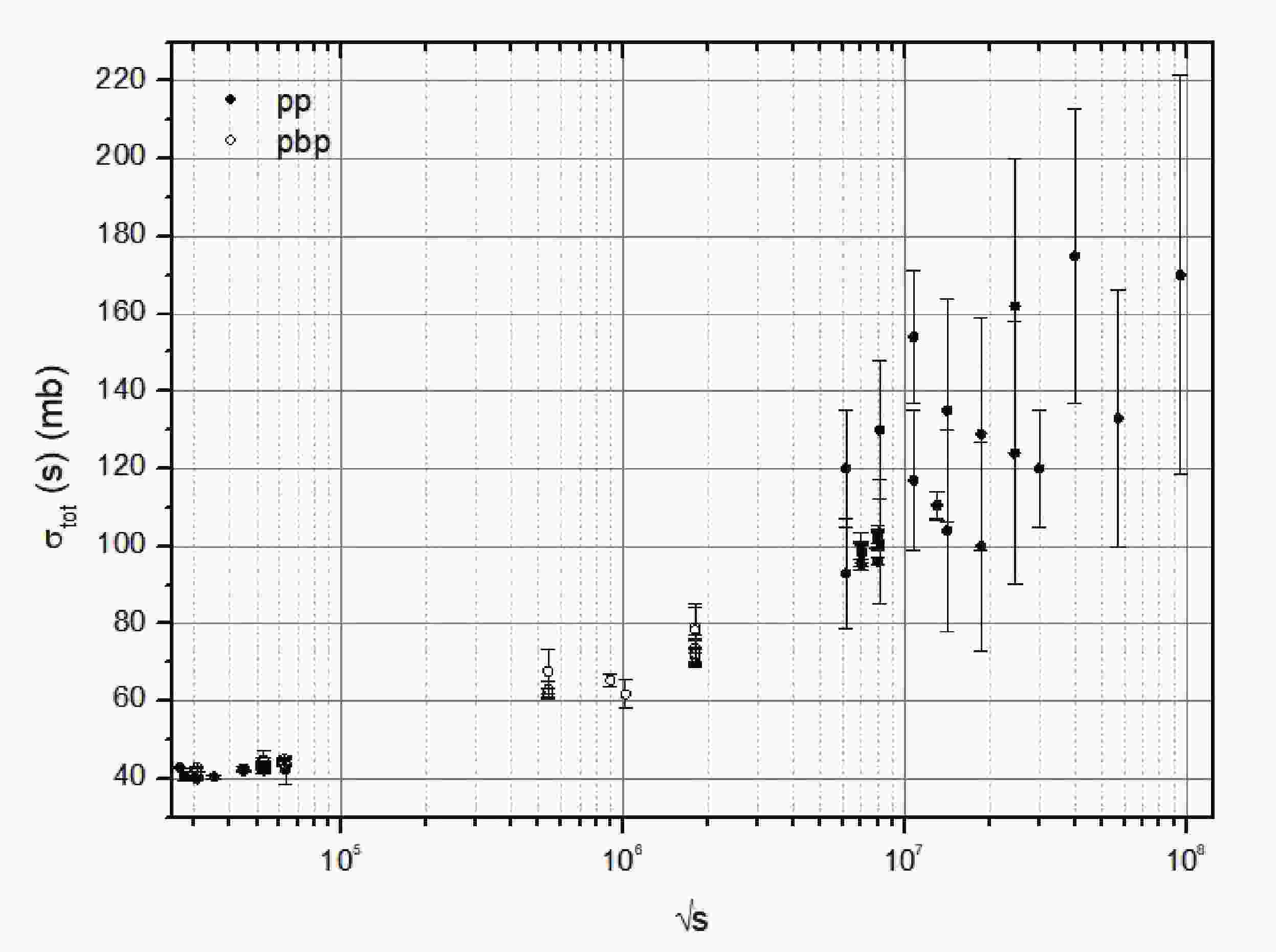
$ pp $ and$ p\bar{p} $ experimental data are used to form a joint data set, as the Pomeranchuk theorem asserts that they tend to the same limit if$ s\rightarrow\infty $ . This behavior, predicted to occur only at the asymptotic regime, seems yet to be started from energies above$ \sqrt{s}\geqslant 25.0 $ GeV. Figure 1 shows the experimental data used in the fitting procedures for$ \sigma_{\rm tot}^{pp}(s) $ and for$ \sigma_{\rm tot}^{p\bar{p}}(s) $ .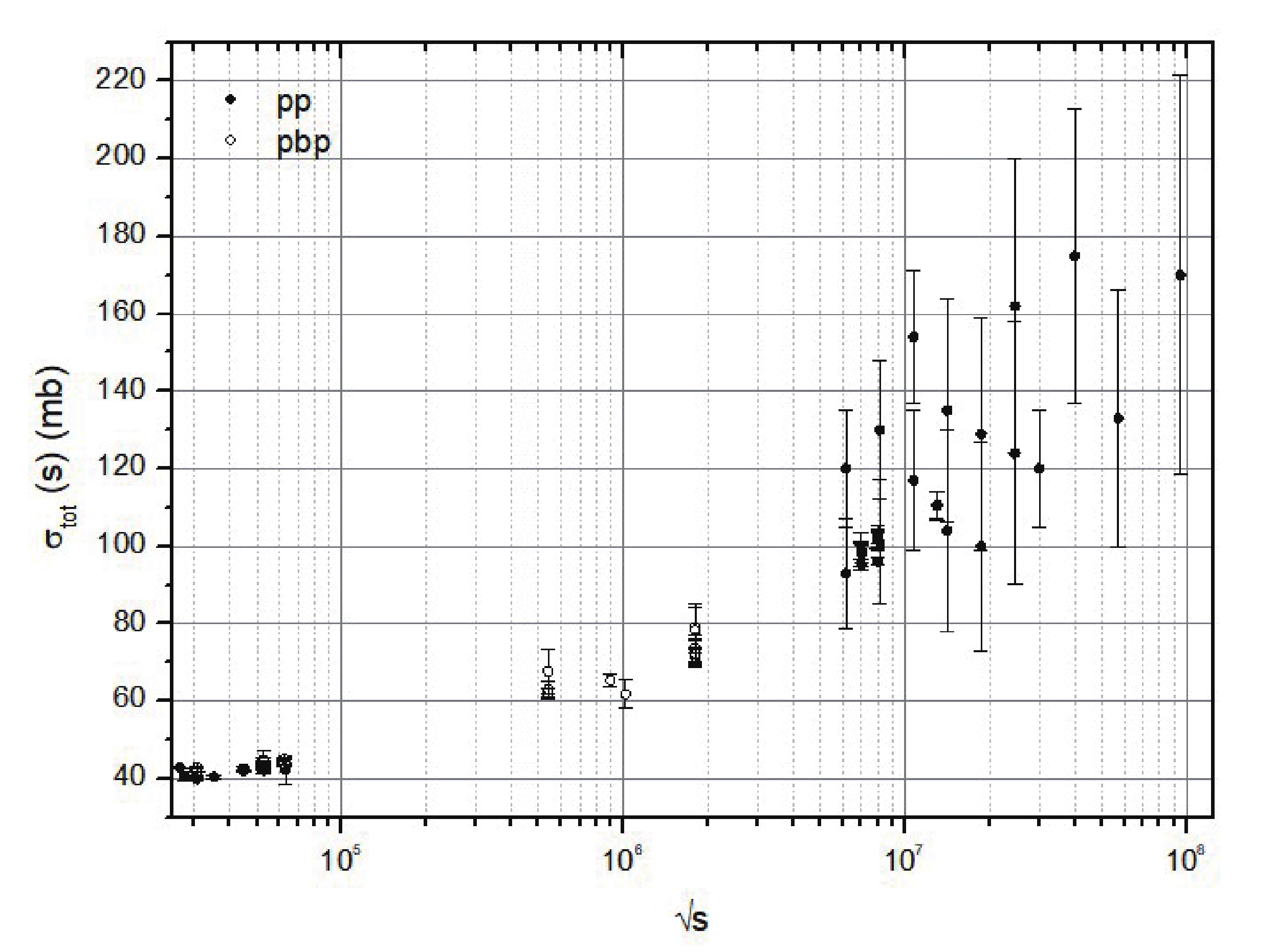
The goal of treating both data sets as one resides on the possibility that the absence of
$ pp $ experimental data, within some energy range, can be compensated by the existence of$ p\bar{p} $ data in this range, and vice-versa. Moreover, there is no data selection in any set considered. The following experimental data set is used throughout this work.● The SET 1 is formed by the experimental data for
$ \sigma_{\rm tot}^{pp}(s) $ and$ \sigma_{\rm tot}^{p\bar{p}}(s) $ above$ \sqrt{s} = 1.0 $ TeV up to the cosmic-ray data.● The SET 2 uses the experimental data for
$ \sigma_{\rm tot}^{pp}(s) $ and$ \sigma_{\rm tot}^{p\bar{p}}(s) $ above$ \sqrt{s} = 1.0 $ TeV, excluding the cosmic-ray experimental data.● The SET 3 contains experimental data for
$ \sigma_{\rm tot}^{pp}(s) $ and$ \sigma_{\rm tot}^{p\bar{p}}(s) $ above$ \sqrt{s_c} $ GeV up to the cosmic-ray data.● The SET 4 excludes the cosmic-ray data from the SET 3.
The energy cut
$ \sqrt{s_c} $ , corresponds to the energy for which the total cross-section achieves its minimum value [32]. For the SET 1 and 2,$ \sqrt{s_c} = 25.0 $ GeV is used. However, as shall be seen, the emergence of a term$ \ln\ln(s/s_c) $ in the logarithmic Regge cut implies a change in$ \sqrt{s_c} $ to avoid the emergence of negative or complex values. Then, for the SET 3 and 4, one uses$ \sqrt{s_c} = 15.0 $ GeV, which is a consequence of the constraint$ \sqrt{s}\geqslant\sqrt{e s_c} $ , where e is the Napier's constant.Using the derivative dispersion relations, the real part of the forward elastic scattering amplitude is obtained. Then, it is possible to present the predictions for the
$ \rho $ -parameter based on the fitting results. We use only the experimental data for$ \rho $ ($ pp $ and$ \bar{p}p $ ) above$ \sqrt{s} = 25.0 $ GeV. It is important to stress that these experimental values were not used in the fitting procedures, i.e., they are used only as a background to show the predictions for the$ \rho $ -parameter. Predictions for the slope of the differential cross-section are also shown, considering some energies of interest. Moreover, a fitting procedure for the slope using the$ pp $ and$ \bar{p}p $ experimental data above 1.0 TeV is performed.All experimental data were collected from the Particle Data Group [30]. Moreover,
$ \sigma_{\rm tot}^{pp}(s) $ at$ \sqrt{s} = 2.76 $ TeV is from [31]. Hereafter, we use only$ \sigma_{\rm tot}(s) $ to refer to both$ \sigma_{\rm tot}^{pp}(s) $ and$ \sigma_{\rm tot}^{p\bar{p}}(s) $ (the same for$ \rho $ ). -
In the Regge theory, the scattering amplitude is written as an analytic function of the angular momentum J. This representation is formulated in the high energy limit
$ s\rightarrow\infty $ and associates the asymptotic behavior of the scattering amplitude in the s-channel to the exchange of one-particle or more, represented in the t-channel by the leading Regge poles. The scattering amplitude is written as$ A(s,t) = {\rm{Re}}A(s,t)+i{\rm{Im}}A(s,t), $

(1) and we also assume that behavior of such a function, at very high energies, is given only by the absorptive part
$ A(s,t)\approx{\rm{Im}}A(s,t) $ . As is well-known, in the usual Regge pole formalism, the asymptotic scattering amplitude is written as$ A(s,t)\rightarrow (\eta+{\rm e}^{-{\rm i}\pi\alpha(t)})\beta(t)(s/s_c)^{\alpha(t)}, \; \; \; s\rightarrow\infty, $

(2) where
$ \eta = \pm 1 $ is the signature related with the crossing symmetry$ s\leftrightarrow t $ ,$ \sqrt{s_c} $ some critical energy, and$ \beta(t) $ is the residue function of the pole depending only on t. In this formalism, s and t are treated as complex-valued functions. Using (2), we attain the asymptotic form of the differential cross-section$ \frac{{\rm d}\sigma}{{\rm d}t}\approx (s/s_c)^{2\alpha(t)}, $

(3) and adopting the normalization
$ s\sigma_{\rm tot}(s) = {\rm{Im}}A (s,t)\approx A(s,t) $ , one has$ \sigma_{\rm tot}(s)\approx (s/s_c)^{\alpha(0)-1}. $

(4) The mathematical disagreement between (4) and the FM bound is given below
$ \sigma_{\rm tot}(s)\leqslant c\ln^2(s/s_c), $

(5) where c is some real constant, inevitable for
$ 1<\alpha(0) $ . However, it is important to stress that the Regge theory predicts both a leading pole behaving as$ (s/s_c)^{\alpha(t)} $ as well as sub-leading terms behaving as$ \ln^k (s/s_c) $ . If$ \alpha(0) = 1 $ in (4), only the logarithmic terms survive, being controlled by the FM bound, which means$ k\leqslant 2 $ . Therefore, the precise knowledge of the leading pole functional form in the Regge approach is subject to experimental evidence.However, the Regge theory and the FM bound can agree with each other if a constraint is imposed on the scattering angle as well as a mathematical approximation on the cosine series [29]. The scattering angle is restricted to the range
$ 0\leqslant \cos \theta \leqslant 1 $ for$ |t|<\!\!< s $ . In this case, the s-channel has the following approximation, valid near the forward direction, for the cosine of the scattering angle [29]$ \cos (\theta) = 1+\frac{2t}{s} \lesssim \ln \left(1+\sqrt{e}\left(1+\frac{2t}{s}\right)\right), $

(6) where physical t is negative,
$ s>4m^2 $ , and m is the particle mass. Importantly, in the s-channel, fixed t represents the squared momentum transfer, and s is the squared energy. Moreover,$ |\cos\theta|\leqslant 1 $ , making it necessary to use the crossing property$ s\leftrightarrow t $ in the high energy limit$ s\rightarrow\infty $ .The approximate representation (6) can be obtained by noting that the usual cosine series can be written as
$ \cos(x) = 1-\sum\limits_{n = 1}^{\infty} \dfrac{(-1)^{n-1}}{(2n)!}x^{2n}, $

(7) where the sum in the r.h.s enclose the information about the energy and momentum transfer. Observing the following inequalities holds for
$ n\in \mathbb{N} $ $ (2n)^{2n+\frac{1}{2}}\geqslant n^{n+\frac{1}{2}}\geqslant n^n\geqslant n. $

(8) Then, the factorial number in (7) can be circumvented using the Stirling's approximation
$ (2n)!\approx (2n)^{2n+\frac{1}{2}}{\rm e}^{-2n}\sqrt{2\pi}. $

(9) Then,
$ \cos(x) = 1-\sum\limits_{n = 1}^{\infty} \frac{(-1)^{n-1}}{(2n)!}x^{2n}\approx 1-\sum\limits_{n = 1}^{\infty} \frac{(-1)^{n-1}{\rm d}^{2n}}{(2n)^{2n+\frac{1}{2}}\sqrt{2\pi}}x^{2n}, $

(10) To reduce the series on the r.h.s. of (7) into logarithmic series, using (8), we can always find a real number a, satisfying
$ \frac{{\rm d}^{2n}}{\sqrt{2\pi}(2n)^{2n+\frac{1}{2}}}\leqslant \frac{a^{2n}}{n}. $

(11) Naturally, the result (11), when replaced in the convenient series, possibly implies a slower convergence than the original cosine series, near the forward direction. Moreover, the choice of a is not unique. For example, the above inequality holds for
$ a = e = 2.71828\cdots $ , where e is the Napier's number.Using the results (9) and (11), the series on r.h.s. of (7) can be exchanged by the approximation
$ \cos(x)\lesssim 1- \sum\limits_{n = 1}^{\infty}\frac{(-1)^{n-1}}{n}[(ax)^2]^n = 1-\sum\limits_{n = 1}^{\infty}\frac{(-1)^{n-1}}{n}[(y)]^n, $

(12) with the condition
$ y\geqslant 0 $ . Using the last result, one finally obtains$ 1-\sum\limits_{n = 1}^{\infty}\frac{(-1)^{n-1}}{n}[(y)]^n = \ln\left(\frac{e}{1+y}\right). $

(13) To ensure the first-order approximation, one uses
$ y = e-\left[1+\sqrt{e}\left(1+\frac{2t}{s}\right)\right], $

(14) where the factor
$ \sqrt{e} $ arises from the fact that$ y\geqslant0 $ . Observing that, for$ t = 0 $ , one has$ \cos\theta = 1 $ , and the approximation performed furnish$ \cos\theta\approx 0.97 $ .Using the asymptotic properties of the Legendre polynomial, taking into account the approximation (6), and the crossing
$ s\leftrightarrow t $ , one writes$ (s\rightarrow\infty $ and fixed t)$ P_l(s)\rightarrow \ln^{l} (s/s_c). $

(15) Indeed, the above result can be used to write the asymptotic scattering amplitude as a logarithmic leading Regge pole
$ A(s,t)\rightarrow \ln^{\alpha(t)}(s/s_c), $

(16) respecting the FM bound.
The very successful model of Donnachie and Landshoff [4], earlier proposed by Badatya and Patnaik [28], describes the hadronic exchanges remarkably well, assuming a simple Regge pole
$ A(s,t) = C(t)s^{1.08+0.25t}, $

(17) where
$ C(t) $ is a constant depending only on t. The corresponding$ \sigma_{\rm tot}(s) $ of such parameterization is written using the optical theorem as$ \sigma_{\rm tot}(s) = C(0)s^{0.08}, $

(18) saturating the FM bound. This Regge pole corresponds to the one-pole exchange, while the double-pole exchange leads to
$ \sigma_{\rm tot}(s)\sim \ln(s/s_c) $ . The intercept of the Regge pole in this model is defined as a linear function$ \alpha(t) = \alpha(0)+\alpha' t, $

(19) where the intercept takes the value
$ \alpha(0) = \alpha_{\mathbb{P}} = 1.08 $ and the slope$ \alpha' = 0.25 $ GeV$ ^{-2} $ .In the language of physics, this intercept corresponds to a soft pomeron - low momentum transfer -
$ \alpha_{\mathbb{P}}\approx 1.05 \sim 1.08 $ . In contrast, the hard pomeron, predicted to mediate diffractive processes - large momentum transfer - has a value$ \alpha_{\mathbb{P}}\approx1.4\sim1.5 $ . This hard pomeron emerges due to the use of the Regge formalism as an analogy to explain the structure-function$ F_2(x,Q^2) $ in terms of the Bjorken scale x and the photon virtuality$ Q^2 $ .Note that both, the one-pomeron exchange in the Donnachie and Landshoff model or the double-pomeron exchange in the logarithmic Regge pole, lead to intercepts
$ \gtrsim 1 $ [4, 29]. However, the one-pomeron exchange with an intercept slightly above 1 violates the FM bound, while for the double-pomeron exchange, this violation only occurs for an intercept above 2. If the intercept is equal 2, then the triple-pomeron exchange is favorable,$ \sigma_{\rm tot}\approx \ln^2(s/s_c) $ . Neither the soft nor the hard pomeron has been discovered to date. -
In [29], one considers only the non-subtraction case. Then, using the optical theorem one has a simple relation for the asymptotic total cross-section
$ \sigma_{\rm tot}(s)\rightarrow \ln^{\alpha_{\mathbb{P}}}(s/s_c). $

(20) In the specified range for
$ \cos(\theta) $ , it respects the FM bound if$ \alpha_{\mathbb{P}}\leqslant 2 $ , providing a physical relation between the pomeron intercept,$ \alpha_{\mathbb{P}} $ , and the saturation of this bound. The soft pomeron, if it exists, is the particle allowing the maximum growth of the total cross-section, obeying the FM bound. As shall be seen, the phenomenology associated with the$ \rho $ -parameter is crucial to obtain the correct pomeron intercept.Using a simple parameterization for the total cross-section
$ \sigma_{\rm tot}(s) = \beta\ln^{\alpha_{\mathbb{P}}}(s/s_c), $

(21) where
$ \beta $ and$ \alpha_{\mathbb{P}} $ are free fitting parameters, we can attain the pomeron intercept. Using the SET 1, we obtain the values for the fitting parameters shown in the first line of the Table 1. Fig. 2(a) shows the curve obtained from the fitting procedure using (21). The intercept agrees with a double-pole pomeron exchange. The fitting results using the SET 2 are shown in the second line of the Table 1. From the statistical point of view, the absence of the cosmic-ray data in the SET 2 practically does not alter the results.SET $ \alpha_{\mathbb{P}} $ 

$ \beta $ /mb

$ \chi^2/ndf $ 

1 1.05 $ \pm $ 0.05

7.54 $ \pm $ 0.92

1.26 2 1.04 $ \pm $ 0.05

7.72 $ \pm $ 0.98

1.31 Table 1. Parameters obtained using (21) in fitting procedures for SET 1 and 2, taking
$ \sqrt{s_c} = 25.0 $ GeV. -
The total cross-section with one subtraction can be written using the following normalization of the optical theorem
$ s\sigma_{\rm tot}(s) = {\rm{Im}}A(s). $

(22) This normalization implies in the logarithmic leading Regge pole
$ \sigma_{\rm tot}(s)\approx \frac{\ln^{\alpha_{\mathbb{P}}}(s/s_c)}{s}. $

(23) First of all, we note that to tame the fast decrease of the total cross-section entailed by the subtraction, it is necessary to have a
$ \alpha_{\mathbb{P}} $ far above from the expected saturation of the FM bound,$ \alpha_{\mathbb{P}}\rightarrow 2 $ . Indeed, to give some physical meaning for$ \alpha_{\mathbb{P}} $ is now a difficult task. The effect of using s in the above result can be observed by adopting the parameterization given below$ \sigma_{\rm tot}(s) = \beta\frac{\ln^{\alpha_{\mathbb{P}}}(s/s_c)}{s}. $

(24) The fitting results obtained using the parameterization (24) to the SET 1 and 2 are shown in Table 2. Naturally, the subtracted case cannot be used as a realistic parameterization to describe the
$ \sigma_{\rm tot}(s) $ . Fig. 2(b) shows the curve obtained from the fitting procedure using (24).SET $ \alpha_{\mathbb{P}} $ 

$ \beta $ /mb

$ \chi^2/ndf $ 

1 11.02 $ \pm $ 0.09

1.99 $ \times 10^{-5}\pm 4.9\times 10^{-6} $ 

5.14 2 10.99 $ \pm $ 0.10

2.15 $ \times 10^{-5}\pm 5.7\times 10^{-6} $ 

5.89 Table 2. Fitting parameters obtained using (24) in fitting procedure to SET 1 and 2, taking
$ \sqrt{s_c} = 25.0 $ GeV.However, if we release the subtraction mechanism by introducing the
$ \delta $ - index as a measurement of the deviation of the non-subtraction to the subtraction case, then one writes the parameterization$ \sigma_{\rm tot}(s) = \beta\frac{\ln^{\alpha_{\mathbb{P}}}(s/s_c)}{s^\delta}. $

(25) Using the SET 1 and 2, we obtain very small values for the
$ \delta $ -index (near zero). In Table 3 displays the fitting parameters. The$ \delta $ -index introduces an error in the fitting parameters higher than the non-subtraction case. However, the central value of each parameter is practically the same. The fitting result is shown in Fig. 3(a).SET $ \alpha_{\mathbb{P}} $ 

$ \beta $ /mb

$ \delta $ 

$ \chi^2/ndf $ 

1 1.05 $ \pm $ 0.82

7.55 $ \pm $ 8.07

0.00 $ \pm $ 0.08

1.29 2 1.04 $ \pm $ 1.07

7.72 $ \pm $ 10.70

0.00 $ \pm $ 0.11

1.77 Table 3. Fitting parameters obtained using (25) in fitting procedure to SET 1 and 2, taking
$ \sqrt{s_c} = 25.0 $ GeV.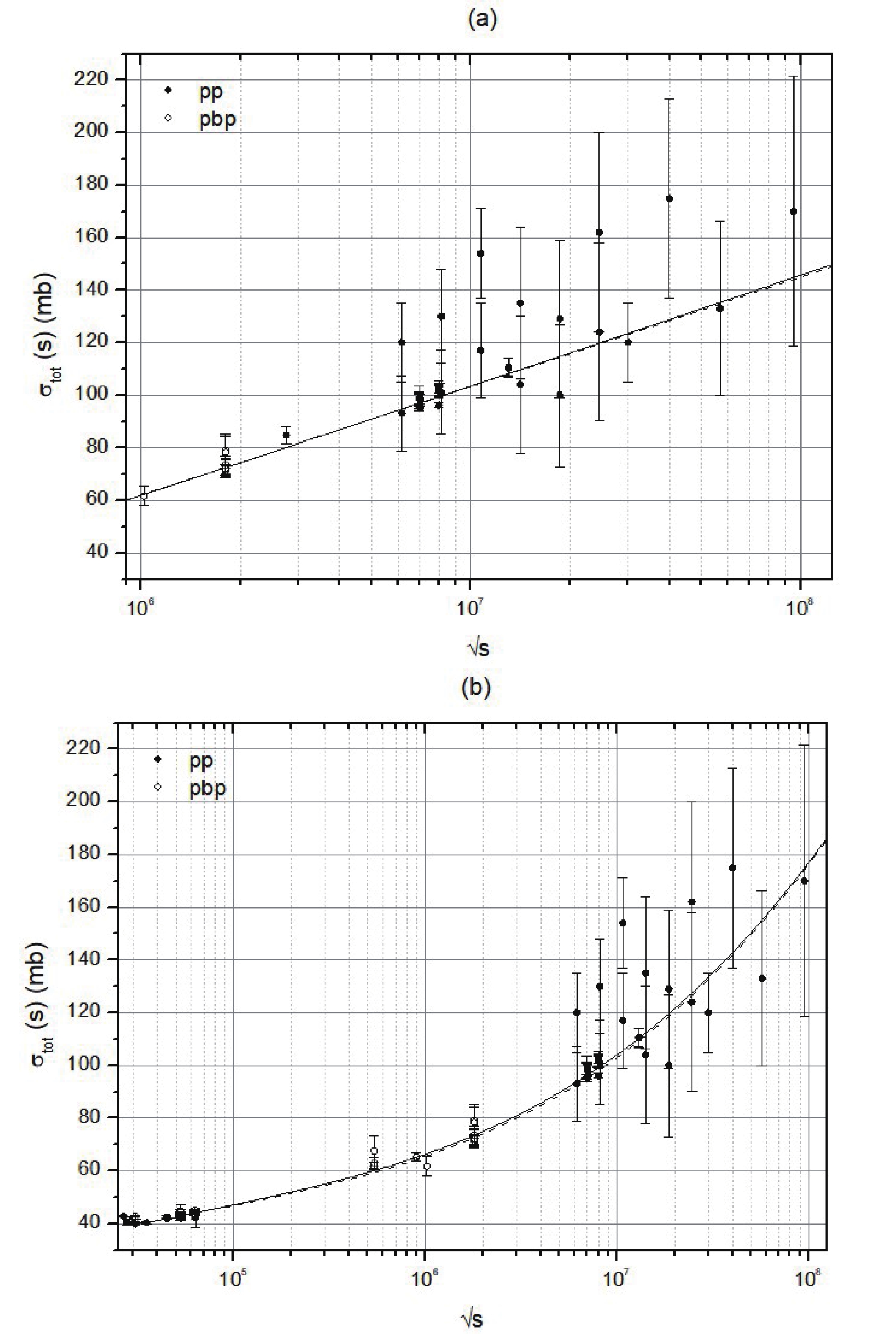
To circumvent the need for the use of the
$ \delta $ -index, we introduce the approximation [29]$ \frac{1}{(s/s_c)^{\delta}}\approx \frac{1}{a(\ln^{\epsilon}(s/s_c))}, $

(26) which is a consequence of the fact that the inequality given below holds for
$ 0<s_c\leqslant s $ and$ 0\leqslant\epsilon\leqslant\delta\in \mathbb{R} $ $ \ln^\epsilon(s/s_c)\leqslant (s/s_c)^\delta\Rightarrow\frac{1}{(s/s_c)^\delta}\leqslant\frac{1}{\ln^\epsilon(s/s_c)}. $

(27) In particular, for some
$ 0<a\in\mathbb{R} $ , the approximation (26) can be used, resulting in the total cross-section$ \sigma_{\rm tot}(s)\approx \beta'\ln^{\alpha_{\mathbb{P}}'}(s/s_c), $

(28) where
$ \alpha_{\mathbb{P}}' = \alpha_{\mathbb{P}}-\epsilon $ and$ \beta' = c/a $ . The choice of a is not unique, and in general, its value depends on the energy range, where the experimental data are being analyzed. However, in the fitting procedure, it is absorbed by$ \beta' $ . Therefore, the expression (28) corresponds to the subtraction case, and it is exactly equal to the non-subtraction case given by (21). -
As is well-known, the singularities play a fundamental role in the determination of the divergences of the partial-wave amplitude. Neglecting the signature of the partial-wave amplitude, one may express the singularities as
$ A_l(t)\propto\int_{\textit{z}}^{\infty}{\rm{disc}}A(s,t)Q_l({\textit{z}}'){\rm d}{\textit{z}}', $

(29) where
$ Q_l({\textit{z}}') $ is the Legendre function of the second kind, and$ {\rm{disc}}A(s,t) $ is the discontinuity across the l-plane cut. The easy way to obtain singularities from (29) is to associate the$ {\rm{disc}}A(s,t) $ with the Legendre function of the first kind,$ P_{\alpha_c(t)}({\textit{z}}) $ , where$ \alpha_c(t) $ is the cut. Then, in the simplest case,$ {\rm{disc}}A(s,t)\propto P_{\alpha_c(t)}({\textit{z}}). $

(30) In this picture, we use the properties of the Legendre functions [33]
$ \int_1^{\infty}P_{\alpha_c(t)}({\textit{z}})Q_l({\textit{z}}){\rm d}{\textit{z}} = \frac{1}{(l+1+\alpha_c(t))(l-\alpha_c(t))}, $

(31) revealing a pole for
$ l = \alpha_c(t) $ ($ l\in\mathbb{R} $ ).The Watson-Sommerfeld representation for the partial-wave expansion in the complex angular plane can be written as
$ A(s,t)_{s\rightarrow\infty}\propto R_p(s,t)+R_c(s,t)+{\rm{vanishing}}\; {\rm{terms}}, $

(32) where
$ R_p(s,t) $ and$ R_c(s,t) $ denote the Regge pole and the Regge cut contributions for the scattering amplitude, respectively. The logarithmic Regge pole introduced in [29] yields the first term in the r.h.s. of (32)$ \begin{split} R_p(s,t)\approx & P_{\alpha(t)}(\cos(\theta))_{s\rightarrow\infty}^{s>>|t|}\longrightarrow \frac{{\rm{\Gamma}}(2l+1)}{{\rm{\Gamma}}^2(l+1)}\ln^{\alpha(t)}(s/s_c)\\ \approx &\ln^{\alpha(t)}(s/s_c). \end{split} $

(33) If a branch point with a cut is encountered during the deformation of the contour in the complex momentum angular plane, then it contributes to the asymptotic behavior of the scattering amplitude. Then, one should take into account the cut contribution. We write
$ R_c(s,t)\propto-\frac{1}{i}\int^{\alpha_{c}(t)}{\rm d}l(2l+1){\rm{disc}}A(l,t)\frac{P_l(-{\textit{z}})}{\sin\pi l}. $

(34) As stated above, the functional form of the discontinuity is not known a priori, and there is no phenomenological approach for it. Therefore, the only way to go through this point is using an ansatz, as performed in Ref. [34].
Using the property
$ {\rm{Im}}P_l({\textit{z}}) = -P_l(-{\textit{z}})\sin\pi l $ ,$ {\textit{z}}<-1 $ , in the logarithmic Regge approach, one adopts$ {\rm{disc}}A (l,t) = (\alpha_c(t)-l)^{1+\beta(t)} $ , obtaining the approximation$ R_c(s,t)\approx-\ln^{\alpha_c(t)}(s/s_c)(\ln\ln(s/s_c))^{-(2+\beta(t))}, $

(35) where
$ -2<\beta(t) $ is a function of t only. Considering the results (33) and (35), the asymptotic scattering amplitude is written as$ A(s,t)\approx \ln^{\alpha(t)}(s/s_c) - \ln^{\alpha_c(t)}(s/s_c)(\ln\ln(s/s_c))^{-(2+\beta(t))}. $

(36) Naturally, the above result is strongly dependent on the form of
$ {\rm{disc}}A(l,t) $ and there is no information about$ \beta(t) $ . The Regge cut$ \alpha_c(t) $ is also an unknown function of t. We suppose here that$ \alpha_c(t) $ and$ \beta(t) $ are real-valued functions, and they assume finite values at$ t = 0 $ .It is important to stress that
$ \sigma_{\rm tot}(s) $ , independently of the functional form of$ {\rm{disc}}A(l,t) $ , must obey the FM bound. Then, the rise of (36) is controlled by$ \ln^2(s/s_c) $ . It is not difficult to see that (hereafter,$ \alpha_c(0) = \alpha_c $ )$ 0\leqslant 1-\ln^{\alpha_c-\alpha_{\mathbb{P}}}(s/s_c)(\ln\ln(s/s_c))^{-(2+\beta(0))}, $

(37) implies that in the asymptotic regime
$ s\rightarrow\infty $ $ \frac{\alpha_c-\alpha_{\mathbb{P}}}{2+\beta(0)}\leqslant 0 \Rightarrow \alpha_c\leqslant \alpha_{\mathbb{P}}, $

(38) for
$ \beta(0)>-2 $ . The inequality$ \alpha_c\leqslant \alpha_{\mathbb{P}} $ implies the Regge cut is bounded by the Regge pole. According to general belief, the subleading (secondary) contributions are important below 1.0 TeV. Then, at ISR energies, the effect of secondary and leading contributions are mixed, while at LHC energies the leading contribution dominates. Therefore, the Regge cut (36) may be used to describe the experimental data behavior from the minimum value of the total cross-section up to$ \sim $ 1.0 TeV, as the role of the cut is now clear: it represents mixed contributions below the logarithmic Regge pole dominance according to inequality (38).To take into account the Regge pole and the Regge cut contributions for the total cross-section, we use the simple parameterization
$ \sigma_{\rm tot}(s) = \beta_1 \ln^{\alpha_{\mathbb{P}}}(s/s_c)-\beta_2\ln^{\alpha_c}(s/s_c)(\ln\ln(s/s_c))^{-(2+\beta(0))}, $

(39) to fit the SET 3 and 4. The fitting results are displayed in Table 4. The Fig. 3(b) shows the curve obtained for the parameterization (39).
SET $\beta_1$ /mb

$\alpha_{\mathbb{P}}$ 

$\beta_2$ /mb

$\alpha_c$ 

$\beta(0)$ 

$\chi^2/ndf$ 

3 0.01 $\pm$ 0.01

3.22 $\pm$ 0.43

−31.32 $\pm$ 1.10

0.32 $\pm$ 0.04

−1.86 $\pm$ 0.02

2.91 4 0.01 $\pm$ 0.01

3.24 $\pm$ 0.50

−31.29 $\pm$ 1.19

0.32 $\pm$ 0.04

−1.86 $\pm$ 0.02

3.36 Table 4. Fitting parameters obtained by (39) in fitting procedure to SET 3 and 4, taking
$\sqrt{s_c}=15.0$ GeV.It is important to stress that there is no constraint on the fitting parameters. Then, one allows the pomeron intercept to assume any value necessary to fit the experimental data. The result, at first glance, shows a pomeron intercept far above the saturation of the FM bound - a supercritical value. Then, a control mechanism must be imposed to tame the growth of the total cross-section as
$ s\rightarrow\infty $ . This control mechanism, as shall be seen, is obtained by looking at the$ \rho $ -parameter experimental data. -
As is well-known, the validity of the Cauchy theorem is crucial for the convergence of the integral dispersion relation. This kind of relationship helps obtain the real part of the forward scattering amplitude from the imaginary part. First of all, one writes the scattering amplitude as the sum of the even (+) and odd (−) amplitudes as
$ A(s,t) = A_+(s,t)\pm A_-(s,t), $

(40) where
$ A_\pm(s,t) = {\rm{Re}}A_\pm(s,t)+i{\rm{Im}}A_\pm(s,t) $ are the crossing even (+) and odd (-) amplitudes. The integral form of the dispersion relations is a consequence of analyticity, unitarity, and crossing properties. In the non-subtraction case, it is simply written as ($ t = 0 $ )$ {\rm{Re}}A_+(s) = \frac{2s}{i}P\int_{s_{\rm min}}^\infty {\rm d}s' \frac{{\rm{Im}}A_+(s')}{s-s'}, $

(41) where P is the principal value of the Cauchy integral. The convergence of the above integral can be ensured using the subtraction procedure, i.e., by rewriting the scattering amplitude as
$ \tilde{A}(s) = \left|\frac{A(s)}{s}\right|, $

(42) which results in the subtraction term
$ {\rm{Re}}\tilde{A}_+(s) = K+\frac{2s^2}{i}P\int_{s_{\rm min}}^\infty {\rm d}s' \frac{{\rm{Im}}\tilde{A}_+(s')}{s(s^2-s'^2)}, $

(43) $ {\rm{Re}}\tilde{A}_-(s) = \frac{2s^2}{i}P\int_{s_{\rm min}}^\infty {\rm d}s' \frac{{\rm{Im}}\tilde{A}_-(s')}{(s^2-s'^2)}, $

(44) where K is the subtraction constant. Naturally, this method is valid only for a finite number of subtractions [35]. However, the integral dispersion relations are very restrictive, because to know the value of the real part to a specific value one should know the value of the imaginary part in the whole plane. Then, despite its rigorous formulation, the use of integral dispersion relations is of little interest in the Regge theory.
In contrast, the derivative dispersion relation can be used in the present case [36, 37]. These derivative relations can be written in the first-order approximation for the odd and even amplitudes as [38]
$ \frac{{\rm{Re}}A_+(s,t)}{s} = \frac{K}{s}+\frac{\pi}{2}\frac{{\rm d}}{{\rm d}\ln s}\frac{{\rm{Im}}A_+(s)}{s}, $

(45) $ \frac{{\rm{Re}}A_-(s,t)}{s} = \frac{\pi}{2}\left(1+\frac{{\rm d}}{{\rm d}\ln s}\right)\frac{{\rm{Im}}A_-(s)}{s}. $

(46) Considering (21) and (39), it is possible to obtain the real part of the scattering amplitude in the subtraction as well as in the Regge cut. Then, the real part of the scattering amplitude can be used to define the
$ \rho $ -parameter$ \rho(s) = \frac{{\rm{Re}}A(s)}{{\rm{Im}}A(s)}. $

(47) Without loss of generality, we set
$ K = 0 $ , as the influence of this parameter is restricted to the low energy region, and the main interest here is to understand the asymptotic regime. Then, all parameters are obtained from the previous fits to the total cross-section.Fig. 4 shows the predictions for the
$ \rho $ -parameter. The results from the logarithmic Regge pole (21) are represented by the dotted line and by the dot-dashed line, SET 1 and 2, respectively. These curves represent the pure contribution arising from the double pomeron exchange. Therefore, these results are not able to reproduce the low energy behavior of the$ \rho $ -parameter. Using the parameterization (39), solid and dashed lines, respectively, display the Regge cut contribution obtained from the fitting procedures for SET 3 and 4. These predictions show behavior in the high energy regime that is not present in experimental data. There is a fast-rise introduced by the experimental data below$ \sqrt{s} = 1.0 $ TeV, which is not present in the experimental data above this energy, because the fittings for the SET 1 and 2 show a pomeron intercept$ \alpha_{\mathbb{P}}\approx 1.05 $ .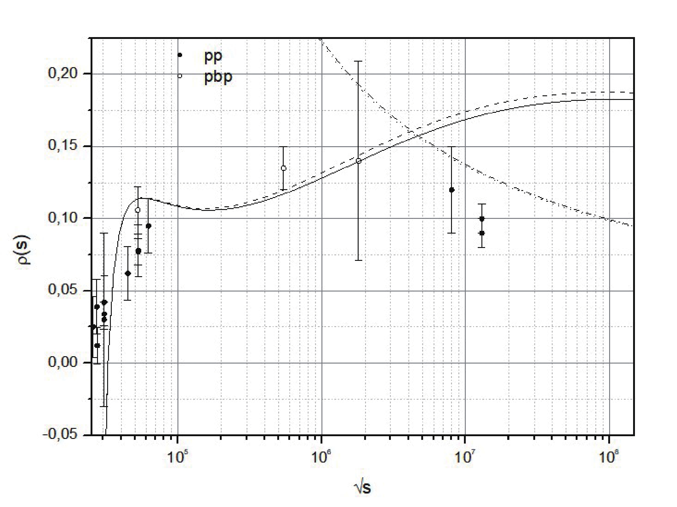
An attempt to solve this problem can be tried using the recent experimental data for the
$ \rho $ -parameter at$ \sqrt{s} = 13.0 $ TeV. These experimental data suggest a double pomeron intercept taming the rise of the total cross-section. Then, considering the above discussion, the constraint$ \alpha_{\mathbb{P}}\leqslant 1 $ can be introduced to reduce the fast-rising of$ \sigma_{\rm tot}(s) $ above 1.0 TeV, introduced by (39). The Table 5 shows the fitting parameters only for SET 3. Despite the high value of$ \chi^2/ndf $ , the fitting parameters seem to be able to reproduce the growth of$ \sigma_{\rm tot}(s) $ as$ s\rightarrow\infty $ .$ \beta_1 $ /mb

$ \alpha_{\mathbb{P}} $ 

$ \beta_2 $ 

$ \alpha_c(0) $ 

$ \beta(0) $ 

$ \chi^2/ndf $ 

6.12 $ \pm $ 5.59

1.00 $ \pm $ 0.27

−30.96 $ \pm $ 3.29

−0.14 $ \pm $ 0.31

−1.92 $ \pm $ 0.04

4.36 Table 5. Fitting parameters obtained by (39) in fitting procedure to SET 3, taking
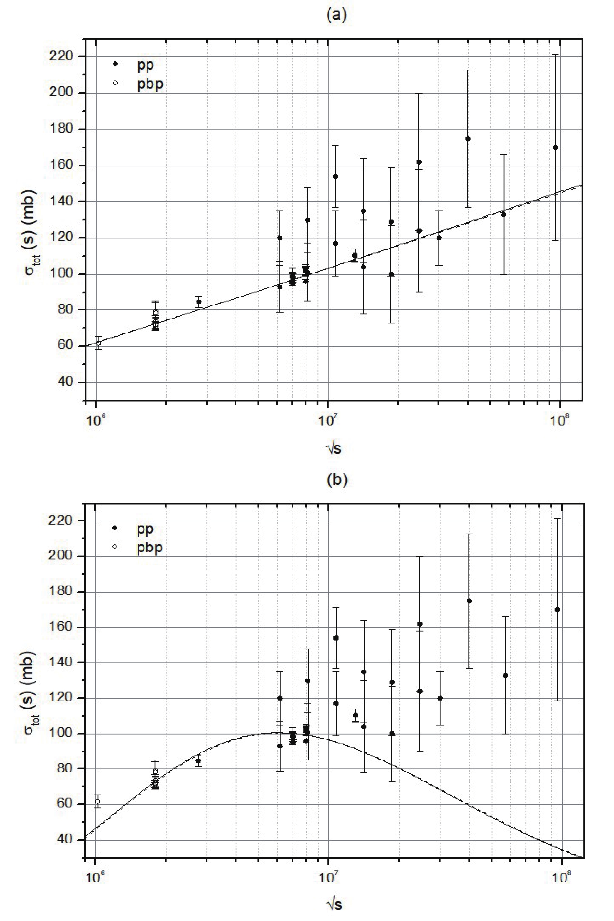
$ \sqrt{s_c} = 15.0 $ GeV and with constraint$ \alpha_{\mathbb{P}}\leqslant 1 $ .The Fig. 5(a) shows the fitting results for
$ \sigma_{\rm tot}(s) $ using the parameterization (39) under the double-pomeron constraint. Fig. 5(b), one shows the prediction for the$ \rho $ -parameter. Despite this naive parameterization, we observe that the only way to reproduce the high energy behavior of$ \rho $ at$ \sqrt{s} = 13.0 $ TeV is assuming a double pomeron exchange in the logarithmic Regge pole representation.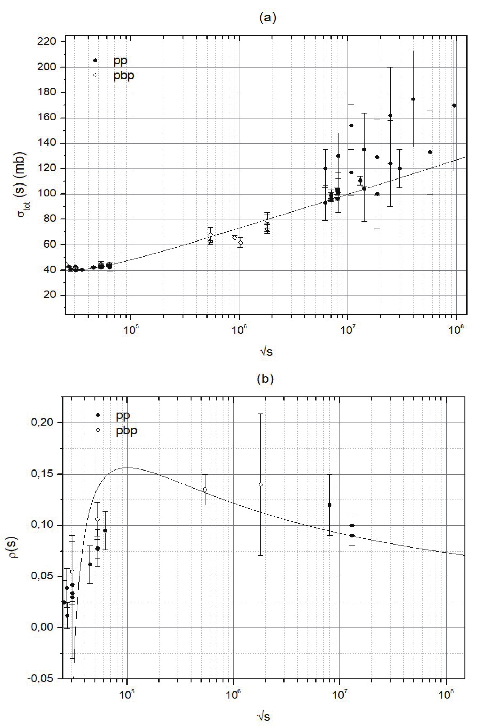
Figure 5. Experimental data are from SET 3 in panel (a), and the parameterization is given by (39) with pomeron constraint
$ \alpha_{\mathbb{P}}\leqslant 1 $ . In panel (b), the prediction for the$ \rho $ -parameter is presented under the double-pomeron constraint.A possible understanding here is that the fast rise of
$ \sigma_{\rm tot}(s) $ in the logarithmic Regge approach cannot be analyzed independently of the$ \rho $ -parameter. In particular, the$ \rho $ value at$ \sqrt{s} = 13.0 $ TeV is crucial to determine an upper bound to the pomeron intercept. It must be stressed that this is a feature of the Regge theory: the phenomenology.Another physical quantity that can be predicted from the fitting procedures performed here is the (forward) slope of the elastic differential cross-section
$ {\rm d}\sigma/{\rm d}t $ , defined as$ B(s,t\rightarrow 0) = \frac{{\rm d}}{{\rm d}t}\left(\ln{\frac{{\rm d}\sigma}{{\rm d}t}}\right)_{t = 0}. $

(48) In the present approach, using the simple asymptotic parameterization (21), for example, one obtains for the forward case
$ B(s) = B_0+2\alpha'\ln(\ln s/s_0), $

(49) where
$ \sqrt{s_0} $ is some initial energy not necessarily related with$ \sqrt{s_c} $ . The value$ s_0 $ can be taken from some current known experimental result for the slope, being used as input to predict the slope at s. For example, using the TOTEM result$ B_0 = 19.9\pm0.3 $ GeV$ ^{-2} $ at$ \sqrt{s_0} = 7.0 $ TeV [39] and$ \alpha' = 0.25 $ GeV$ ^{-2} $ , we have the prediction for the elastic slope$ B(s) = 20.0\pm0.3 $ GeV$ ^{-2} $ at$ \sqrt{s} = 13.0 $ TeV. As is well-known, the LHC result at$ \sqrt{s} = 13.0 $ TeV is$ B(s) = 20.36\pm0.19 $ GeV$ ^{-2} $ [31], in accordance with the value predicted here. In contrast, starting from the TOTEM result, one cannot reproduce, for example, the unexpected value for the slope encountered by the E710 Collaboration at$ \sqrt{s} = 1.8 $ TeV,$ B(s) = 16.98\pm0.25 $ GeV$ ^{-2} $ [40].The prediction capability of (49) is, evidently, limited by the constraint
$ \sqrt{s}\geqslant\sqrt{e s_0} $ . This implies, for example, that the next energy above the LHC at$ \sqrt{s} = 13.0 $ TeV can predict the slope at$ \sqrt{s}\approx 22 $ TeV (likewise for the$ \rho $ -parameter). Therefore, using the LHC result as the initial value$ \sqrt{s_0} = 13.0 $ TeV, we obtain$ B(s) = 20.38 $ GeV$ ^{-2} $ at$ \sqrt{s} = 22.0 $ TeV, indicating a very slow increase for the slope. At the same energy, the slope from the usual leading Regge pole is$ B(s) = 20.88 $ GeV$ ^{-2} $ .In contrast, if instead of (21), we use the parameterization considering the logarithmic Regge cut (39), then for the slope in the forward case,
$ B(s) = B_0+3[(\alpha'+\alpha_c'(0))\ln(\ln s/s_0)-\beta'(0)\ln(\ln(\ln s/s_0))]. $

(50) Evidently, the importance of the factor
$ \ln(\ln(\ln s/s_0)) $ in the r.h.s. of the above result depends strongly on the values of s and$ s_0 $ . For example, from the E710 to the TOTEM energy, we obtain$ \ln(\ln(\ln s/s_0)) = -7.49\times 10^{-4} $ , while from the TOTEM to the LHC,$ \ln (\ln(\ln s/s_0)) = -1.54 $ . Therefore, we set, for the sake of simplicity,$ \beta'(0) = 0 $ . Then, we express the slope as$ B(s)\approx B_0+3(\alpha'+\alpha_c'(0))\ln(\ln s/s_0). $

(51) The parameter
$ \alpha_c'(0) $ is unknown and strongly influences the slope. For example, using the TOTEM result$ B_0 = 19.9\pm0.3 $ GeV$ ^{-2} $ at$ \sqrt{s_0} = 7.0 $ TeV and taking$ \alpha_c'(0) = 0.25 $ GeV$ ^{-2} $ , we obtain the LHC result at$ \sqrt{s} = 13.0 $ TeV,$ B(s) = 20.22\pm0.3 $ GeV$ ^{-2} $ . Furthermore, using the E710 experimental result and$ \alpha_c'(0) = 0.25 $ GeV$ ^{-2} $ , we have$ B(s) = 18.47\pm 0.25 $ GeV$ ^{-2} $ for the TOTEM at$ \sqrt{s} = 7.0 $ TeV.However, setting
$ \alpha_c'(0) = 0.50 $ GeV$ ^{-2} $ and starting from the TOTEM energy, then for the LHC at$ \sqrt{s} = 13.0 $ TeV, we obtain$ B(s) = 20.38\pm0.3 $ GeV$ ^{-2} $ . Nonetheless, using the E710 at$ \sqrt{s} = 1.8 $ TeV and the TOTEM at$ \sqrt{s} = 7.0 $ TeV, then the slope is$ B(s) = 19.22\pm0.25 $ GeV$ ^{-2} $ . The last result is better than using$ \alpha_c'(0) = 0.25 $ GeV$ ^{-2} $ , but still below the TOTEM result.In contrast, assuming
$ B_0 $ and$ \alpha_c'(0) $ as free parameters, and setting$ \alpha' = 0.25 $ GeV$ ^{-2} $ and$ \sqrt{s_0} = 15.0 $ GeV,we can fit the experimental data for the slope above 1.0 TeV ($ pp $ and$ p\bar{p} $ ). In this energy range, the slope seems to be a linear function of s, and therefore, we can use the result (51) to fit these experimental data [30]. Thus, we obtain$ \alpha_c'(0) = 2.91\pm 0.25 $ GeV$ ^{-2} $ and$ B_0 = -3.51\pm 1.73 $ GeV$ ^{-2} $ .It is interesting to note that it is a very difficult task to access the slope
$ B(s) $ , since it is not extracted at$ t = 0 $ . In general, the slope is obtained considering very small ranges of$ t\approx 0 $ , which implies Coulomb and Nuclear contributions to the scattering amplitude. For example, for the E710 Collaboration [40], the interval for t is$ [0.04, 0.29] $ GeV$ ^2 $ and for the TOTEM Collaboration, one has$ t\in[0.012, 0.2] $ GeV$ ^2 $ [31]. Then, these experimental values may carry some dependence on the momentum transfer. -
We obtain the leading Regge pole with one subtraction as well as the Regge cut, both in the logarithmic representation introduced previously in [29]. The fitting procedures for the subtraction case led to unrealistic results to
$ \sigma_{\rm tot}(s) $ , i.e., to a decrease that is faster than the rise of the experimental data, rendering the subtraction a problem in the logarithmic Regge pole.By attempting to understand this problem, we introduce a small parameter, the
$ \delta $ -index, to determine the strength of subtraction in this approach. The fitting procedures indicate a$ \delta $ -index value near to zero (a very weak dependence on the subtraction). This result allowed the use of a logarithmic representation for the subtraction. Then, the subtraction and the non-subtraction cases can be described by the same logarithmic Regge pole.The fitting procedures considering only energies above 1.0 TeV result in a pomeron intercept compatible with the double-pomeron value,
$ \alpha_{\mathbb{P}}\approx 1.04\sim1.05 $ . This value corroborates the Double-Logarithmic contributions, indicating that the higher accuracy of calculations, the lower the intercept, resulting in the best value given by the intercept close to 1 [41, 42].The Regge cut in the original Regge formalism does not have a clear role. However, in the present approach, the logarithmic Regge cut may represent the contributions coming from below the logarithmic Regge pole,
$ \alpha_{\mathbb{P}} $ , when one adopts$ {\rm{disc}}A(l,t) = (\alpha_c(t)-l)^{1+\beta(t)} $ . Then, it can be used to explain the mixed region ($ 25.0 \; {\rm{GeV}} \leqslant \sqrt{s}\leqslant 1.0 \; {\rm{TeV}} $ ), where the odderon and the pomeron compete as the leading contribution to the total cross-section.Here, we expect that logarithmic Regge cut can describe the total cross-section for
$ pp $ and$ p\bar{p} $ , from the minimum of the total cross-section up to 1.0 TeV. However, assuming the parameters coming from the Regge cut can act as free fitting parameters, then they cause a supercritical value to the pomeron intercept, leading to the saturation of the FM bound. Notwithstanding, the dominance of the pomeron as the leading contribution at LHC energy seems to be an experimental fact [43]. It is important to stress that the fitting procedures for SET 1 and 2, using the parameterization (21), furnish an important constraint on the pomeron intercept$ \alpha_{\mathbb{P}} $ . Moreover, the experimental data at the cosmic-ray energies seem to have little influence on the pomeron intercept.To solve this problem, it is necessary to use the experimental data for the
$ \rho $ -parameter. In particular, one should use the experimental result at$ \sqrt{s} = 13.0 $ TeV. This value seems to impose a double pomeron exchange, resulting in an intercept$ \alpha_{\mathbb{P}}\leqslant 1 $ . When this experimental fact is used, then$ \sigma_{\rm tot}(s) $ rises below the saturation of the FM bound. By all means, as stated in [18], the values for the$ \rho $ -parameter at$ \sqrt{s} = 13.0 $ TeV excluded all the models classified and published by COMPETE. Therefore, the slowing down of the$ \sigma_{\rm tot}(s) $ seems to be given by the$ \rho $ -parameter at$ \sqrt{s} = 13.0 $ TeV.The slope of the differential cross-section can also be predicted by the logarithmic Regge pole. Using the slope obtained by the TOTEM Collaboration, one predicts
$ B(\sqrt{s} = 13.0\; {\rm{TeV}}) = 20.0\pm0.3 $ GeV$ ^{-2} $ , which is in accordance with the result obtained by the LHC,$ B(\sqrt{s} = 13.0\; {\rm{TeV}}) = 20.36\pm0.19 $ GeV$ ^{-2} $ .In the logarithmic Regge pole approach presented here, the Regge cut seems to have a clear role: it spans the mixed region (
$ 25.0\; {\rm{GeV}}\lesssim \sqrt{s}\lesssim 1.0\; {\rm{TeV}} $ ), where the total cross-section can be described by the odderon and pomeron contributions. However, this result is strongly dependent on the discontinuities of the scattering amplitude. Unfortunately, there is no theoretical nor phenomenological information about the discontinuity of$ A(l,t) $ .SDC thanks UFSCar for the financial support.
Logarithmic Regge pole
- Received Date: 2020-04-28
- Available Online: 2020-10-01
Abstract: This work presents the subtraction procedure and the Regge cut in the logarithmic Regge pole approach. The subtraction mechanism leads to the same asymptotic behavior as previously obtained in the non-subtraction case. The Regge cut, in contrast, introduces a clear role to the non-leading contributions for the asymptotic behavior of the total cross-section. From these results, some simple parameterization is introduced to fit the experimental data for the proton-proton and antiproton-proton total cross-section above some minimum value up to the cosmic-ray. The fit parameters obtained are used to present predictions for the


 DownLoad: