


 Abstract
 HTML
HTML Reference
 Related
 PDF
PDF


-
In mainstream inflationary theory, curvature perturbations are generated by inflationary perturbations seeding temperature fluctuations in the cosmic microwave background. However, this broad class of theories is strongly determined by the shape of the inflationary potential. To relax this stringent condition, many alternative mechanisms have been proposed. The curvaton mechanism is one such model; the curvaton field featuring in this mechnism is an additional scalar field that is subdominant during inflation. After inflation, the density of curvatons becomes increasingly significant; this generates curvature perturbations exceeding those arising from inflation [1-3].
All standard model (SM) come from preheating or reheating period [4-10]. In particular, for the narrow resonance case, Ref. [6] presents a general discussion within the framework of the Wentzel–Kramers–Brillouin (WKB) approximation. The reheating temperature is not sufficient to permit coupling between the inflaton and other SM particles; thus, a preheating process is mandatory [11] in certain inflationary models. Most of these models posit a perturbative curvaton decay once inflation has completed [12]. However, the non-perturbative decay of curvatons has also been suggested [13]. Moreover, the curvaton can be dubbed as a source to generate amount of gravitational waves (GW) during preheating [14]. Because of the rich phenomena associated with curvatons, they can be embedded into multi-field frameworks [15].
Curvatons might couple to the Higgs field; if so, the curvaton mass can vary significantly [16, 17]. In this paper, we propose a similar idea; that is, we consider a coupling between the inflaton and the curvaton fields, through which the curvaton mass can be varied. Generally, curvaton decay occurs when the curvaton decay rate
$ \Gamma_\chi $ approaches the Hubble parameter H. Relaxing the condition that the curvaton condensate dominates over its perturbations could yield large local non-Gaussianities [18]. However, current observations [19] severely constrain these models: the (local) non-Gaussianity$ f_{NL} $ cannot be too large ($ |f_{NL}|< 10 $ ), ruling out curvaton models that produce large non-Gaussianities. However, this local type of non-Gaussianity can be suppressed by a quadratic plus quartic potential [20] or by a string axionic potential [21, 22]. Taking the local non-Gaussianity into account will strongly constrain the curvaton decay; for more details on the so-called "fraction of curvaton energy density" during the radiation period, please see the recent investigations described in [23].The curvaton field is generally regarded as an independent additional scalar field to the inflaton field. Thus, curvatons could play the roles of various particles (e.g., axions [24]), to account for dark matter (DM). Because of these axion roles, the curvaton could also produce axionic-primordial blackholes [25, 26]; in some sense, this explains DM. Furthermore, primordial blackholes acting as DM could be generated by curvaton and inflaton mixed models [27].
In the traditional curvaton scenario, curvature perturbation are generated after inflation because the curvaton outlives the inflaton. Meanwhile, the main contribution to curvature perturbations arises from the balance between the curvaton and inflaton; is considered as an assumption for curvaton mechanisms. In our model, the curvaton field is generated by the inflaton decay; this entails a direct coupling between the curvaton and inflaton fields. For this scenario, we treat the curvaton potential as containing a coupling term that dominates and an exponential term that mimicks the dynamical behavior of dark energy. When the curvaton decays into other particles (
$ i.e. $ , Higgs particles,$ W^{\pm} $ $ e.t.c $ ), its potential approaches a constant value, which is considered to play the role of a cosmological constant. In some sense, our scenario could account for the origin of dark energy from a phenomenological perspective. Therefore, we comprehensively analyze the curvaton, from its generation during the inflationary period up to the very late Universe (i.e., up to the present dark energy epoch).This paper is organized as follows. In Section 2, we introduce our inflationary model with its two scalars: the inflaton and the curvaton. The curvaton potential contains two terms: a coupling term (between the curvaton and inflaton) and an exponential term. In Section 3, we describe the curvaton's production through inflaton decay, in terms of parametric resonance preheating. In Section 4, the detailed power spectrum calculation and corresponding local non-Gaussianity are given in the
$ \delta N $ formalism. In Section 5, we illustrate how dark energy is generated from the exponential potential of the curvaton, from a phenomenological perspective. Finally, Section 6 concludes the paper.We work in natural units, in which
$ c = 1 = \hbar $ ; however, we retain the Newton constant G. -
The (p)reheating process provides a mechanism for generating particles and also produces entropy perturbations. An essential component of the preheating process is the parametric resonance, which requires a coupling between the inflaton field and another field. Because the (p)reheating mechanism is rather crude, numerous heuristic approaches have been used to investigate it.
To realize the curvaton mechanism within the framework of preheating, Ref. [28] presented a numerical study of the curvature perturbations produced by the entropic field; this can be regarded as a particular realization of the curvaton mechanism during the preheating process. Thus, it becomes possible to directly construct a curvaton scenario. Subsequently, to account for the origin of dark energy, we assume that the second term of the curvaton potential is of exponential form. Therefore, the total action can be constructed as follows:
$ \begin{split} S =& \int {\rm d}^{4}x\sqrt{-g}\Bigg\{\frac{M_{P}^{2}}{2}R-\frac{1}{2}g^{\mu\nu}\nabla_{{{\mu}}}\phi\nabla_{\nu}\phi-\frac{1}{2}g^{\mu\nu}\nabla_{{{\mu}}}\chi\nabla_{\nu}\chi \\&-V(\phi)-\frac{g_0}{M_{P}^{2}}\chi^{2}V(\phi)-\lambda_{0}\exp\left[-\lambda_{1}\frac{\chi}{M_{P}}\right]\Bigg\}, \end{split}$

(1) where
$ \chi $ and$ \phi $ denote the curvaton and inflaton, respectively; R denotes the Ricci scalar; g is the determinant of$ g_{\mu\nu} $ ; and$ g_0 $ ,$ \lambda_0 $ , and$ \lambda_1 $ are dimensionless parameters determined by the Lagrangian.To better understand this scenario, we further elaborate the action expressed in Eq. (1). In some sense, the curvaton could be produced via the inflaton decay [29]; however, the branching ratio cannot be too large. In the following, we illustrate the curvaton's production via parametric resonance in preheating processes.
-
The curvaton field is generated by parametric resonance. Generally, the curvaton production mechanism includes two terms: the background (considered as a classical field) and the quantum fluctuations of the curvaton. For simplicity, we focus on the main contribution of the background field, assuming it to depend only on time.
We follow the standard procedure described in [5, 9]. First, we require the equation of motion (EoM) for the curvaton field
$ \chi $ ; by varying the action (Eq. (1)), we obtain the EoM of the background$ \chi $ field as$ \ddot{\tilde{\chi}}+\frac{g_0}{M_{P}^{2}}m^{2}\phi^{2}\tilde{\chi} -\frac{\lambda_{0}\lambda_{1}}{M_{p}}\left[1-\lambda_{1}\frac{\tilde{\chi}}{M_{P}}\right]\approx0, $

(2) where the variable substitution
$ \tilde{\chi} = a^{3/2}\chi $ was used and the term$ \dfrac{9}{4}H^{2}\tilde{\chi}+\dfrac{3}{2}\dot{H}\tilde{\chi} $ was neglected. To solve Eq. (2), the background solution for$ \phi $ is required. Its EoM is derived using$ \ddot{\phi}+3H\dot{\phi}+\frac{{\rm d}V(\phi)}{{\rm d}\phi} = 0, $

(3) where
$\partial_{\phi}V = \partial_{\phi}\left(\dfrac{1}{2}m^{2}\phi^{2}+\dfrac{1}{2}\dfrac{g_0}{M_{P}^{2}}\chi^{2}m^{2}\phi^{2}\right)$ . Here, we define the effective mass of the inflaton as$m_{\rm eff}^{2} = m^{2}+\dfrac{g_0}{M_{P}^{2}}\chi^{2}m^{2}$ , which means that$m_{\rm eff}\approx m, \partial_{\phi}V = m_{\rm eff}^{2}\phi$ when$ \dfrac{g_0}{M_{P}^{2}}\chi^{2}\ll 1 $ , as illustrated in Fig. 1. As seen in the derivation of Eq. (2), we neglect$ \dfrac{9}{4}H^{2}\tilde{\chi}+\dfrac{3}{2}\dot{H}\tilde{\chi} $ . Later on, we will show that this is a rational assumption. Meanwhile, making the variable substitution$ \tilde{\phi}(t) = a^{3/2}\phi(t) $ (where a is a scale factor) and implementing the same trick as was used for deriving Eq. (2), Eq. (3) becomes
Figure 1. (color online) Density plot of spectral index (12): The horizontal line corresponds to the e-folding number N, whose range is
$ 50\leqslant N\leqslant60 $ . The vertical line denotes the value of$ g_0 $ , which varies from$ 0.000001 $ to$ 0.023 $ . The right-hand panel matches the value of$ n_\chi $ to its corresponding color.$ \ddot{\tilde{\phi}}+m_{\rm eff}^{2}\tilde{\phi} = 0, $

(4) for which the solution is
$ \phi(t) = a^{-3/2}\cos(m_{\rm eff} t). $

(5) We plug Eq. (5) into Eq. (2) and rearrange the result; after some calculation, this equation becomes
$ \begin{split} \ddot{\tilde{\chi}}&+\frac{g_0m^{2}}{2M_{P}^{2}}\phi_{0}^{2}\tilde{\chi}a^{-3}+\frac{m^{2}g_0}{2M_{P}^{2}}\tilde{\chi}\phi_{0}^{2}a^{-3}\cos(2m_{\rm eff}t)\\&+\frac{\lambda_{0}\lambda_{1}^{2}}{M_{p}^{2}}\tilde{\chi} = \lambda_{0}\lambda_{1}/M_{P}. \end{split}$

(6) Thereafter, we set
$z = m_{\rm eff}t$ ; thus, Eq. (6) becomes$ \begin{split} \tilde{\chi}''&+\frac{g_0}{2M_{P}^{2}}\phi_{0}^{2}\tilde{\chi}a^{-3}+\frac{g_0}{2M_{P}^{2}}\phi_{0}^{2}\tilde{\chi}a^{-3}\cos(2z)\\&+\frac{\lambda_{0}\lambda_{1}^{2}}{m_{\rm eff}^{2}M_{p}^{2}}\tilde{\chi} = \lambda_{0}\lambda_{1}/(m_{\rm eff}^{2}M_{P}), \end{split} $

(7) where we have used the approximation
$m_{\rm eff}\approx m$ , and$\tilde{\chi}' = \dfrac{{\rm d}\tilde{\chi}}{{\rm d} z}$ . Next, following the notation of Ref. [6], we write the standard form as$ \tilde{\chi}''+(A_{k}+2q_{k}\cos[2z])\tilde{\chi} = c , $

(8) where
$c = \lambda_{0}\lambda_{1}/(m_{\rm eff}^{2}M_{P})$ ; subsequently, we compute the correspondence as follows:$ A_{k} = \frac{g_0\phi_{0}^{2}}{2M_{P}^{2}}a^{-3}+\frac{\lambda_{0}\lambda_{1}^{2}}{m_{\rm eff}^{2}M_{p}^{2}}, $

(9) $ q_{k} = \frac{\phi_{0}^{2}g_0}{2M_{P}^{2}}a^{-3}. $

(10) As described in Section 2, the exponential potential
$ \lambda_0\exp \left(-\lambda_1\dfrac{\chi}{M_P}\right) $ mimicks the evolution of dark energy; thus, the$ \chi $ field approaches zero and$ \lambda_0 $ is determined to be of the same order as dark energy. By comparing this to the other terms in Eq. (8), we can set$ c\approx 0 $ . To identify the range of q, we analyse the spectral index of the curvaton; detailed calculations are shown in the Appendix. The formula for the curvaton's spectral index is as follows:$ n_\chi = -2\epsilon_1-\eta_c , $

(11) where
$ \epsilon_1 $ and$ \eta_c $ are defined in Eqs. (47) and (50), respectively; the spectral index is expressed in terms of the leading orders of slow-roll parameters. We assume that the slow-roll conditions apply to the inflaton and curvaton. In the curvaton scenario, the inflaton energy density dominates before it decays into the curvaton; this is also an assumption for the curvaton mechanism. Consequently, the value of the Hubble parameter is strongly determined by inflation. Then, the slow-roll approximation of inflation is adopted, through which we derive that$\epsilon_1 = \epsilon_V = \dfrac{M_P^2}{2}\bigg(\dfrac{V'}{V}\bigg)^2$ , where$ V' = \dfrac{\partial_V}{\partial_\phi} $ . Because$ N\approx \dfrac{\phi^2_*}{4M_p^2} $ , we can easily compute that$ \epsilon_1 = \dfrac{1}{N} $ . Because$ \eta = -\dfrac{2}{3}\dfrac{V''(\chi)}{H^2} $ , we can also implement the slow-roll approximation and focus on the$ V''(\chi) = \dfrac{\partial^2 V(\chi)}{\partial \phi^2} $ term. Subsequently, we find that$ \eta_ = -4g_0 $ , irrespective of the inflation model. Thus, by combining these two parts, we deduce that$ n_\chi = -\frac{1}{N}+4g_0, $

(12) where N denotes the e-folding number. From this equation, we can see the varying trends of
$ n_\chi $ in Fig. 1; furthermore, using the observational constraint of$ n_\chi\approx 0.035 $ from [30], the value of$ g_0\approx 0.013 $ can be determined as being of order$ 10^{-2} $ .The value of the spectral index
$ n_\chi $ is strongly determined in a large class of inflationary models; in these models, the e-folding number depends only on the type of slow-roll inflation [31]. In some sense,$ n_\chi $ is independent of inflation. From another perspective,$ g_0 $ is determined by this constraint. In Eq. (10), it can be seen that q is also determined by$ \phi_0 $ , where it represents the amplitude of the inflaton field. When inflation ends, the value of$ \phi_0 $ could be of order unity. If so, q will be of order unity as well. When$ q_k\ll 1 $ and$ q_k\geqslant 1 $ , Eq. (8) can be treated in terms of narrow resonance and broad resonance cases, respectively. -
In this case,
$ q_k\ll 1 $ , which means that$ g_0\phi_0^2\ll 2M_P^2 $ . Ref. [6] provides a general framework for considering narrow parametric resonance. The crucial physical quantities are the decay rate$ \Gamma_\chi $ and the number density of resonance$N_{\rm res}$ .$ \Gamma_\chi $ denotes the quantity of energy transferred to the curvaton field.$N_{\rm res}$ represents the number density of curvatons.From Ref. [6], we directly extract the formulas for
$ \Gamma_\chi $ and$N_{\rm res}$ $ N_{\rm res} = \sinh^{2}\bigg(\frac{\pi g_{n}^{2}}{2\Gamma_{\chi}\omega_{\rm res}^{3}}\bigg), $

(13) $ \Gamma_{\chi} = \frac{\pi g_{n}^{2}}{\omega_{\rm res}^{3}}\ln^{-1}\bigg(\frac{32\pi^{2}\rho}{\omega_{\rm res}^{4}}\bigg), $

(14) where
$ \rho = \dfrac{1}{2}m^{2}\phi^{2} $ , and n denotes the n-th band of the periodic function; here,$ g_1 = g_{1} = \dfrac{g_0}{2M_{P}^{2}a^{-3}} $ and$\omega_{\rm res} = \dfrac{1}{2}m_{\rm eff} = \frac{1}{2}\omega$ . To acheive efficient curvaton production, we require that$N_{\rm res}\gg 1$ . As a consequence, it is simply concluded that$32\pi^{2}\rho\gg\omega_{\rm res}^{4}$ , which means that the initial value of$ \phi $ considerably exceeds its mass (more specifically, its effective mass); this is consistent with the conditions of chaotic inflation [32]. Namely, efficient production requires a large inflaton field. -
The theoretical framework described in [5, 9] provides a general method for studying the broad resonance case corresponding to
$ q_k\geqslant 1 $ . First, the standard equation can be written as$ \ddot{\tilde{\chi}}+\omega^{2}\tilde{\chi} = 0, $

(15) where
$ \omega^{2} = +\frac{g_0m^{2}}{2M_{P}^{2}}\phi_{0}^{2}a^{-3}+\frac{m^{2}g_0}{2M_{P}^{2}}\phi_{0}^{2}a^{-3}\cos(2m_{\rm eff}t)+\frac{\lambda_{0}\lambda_{1}^{2}}{M_{p}^{2}} , $

(16) and
$\dot{\tilde{\chi}} = \dfrac{{\rm d}\tilde{\chi}}{{\rm d}t}$ . Though particles are produced in highly non-equilibrium processes, we can still use the$ WKB $ approximation to analytically solve Eq. (16); for this, we use the assumption of an adiabatic process operating within a very short time interval, from$ t_i $ to$ t_{i+1} $ . The general solution under the WKB approximation is$ \tilde{\chi}_k^{wkb}\approx\frac{\alpha_{k}}{\sqrt{2\omega}}{\rm e}^{-{\rm i}\int^{t}\omega {\rm d}t}+\frac{\beta_{k}}{\sqrt{2\omega}}{\rm e}^{{\rm i}\int^{t}\omega {\rm d}t} , $

(17) where
$ \alpha_k $ and$ \beta_k $ are constant under the aforementioned assumption, and$ \big|\alpha_{k}\big|^{2}-\big|\beta_{k}\big|^{2} = 1 $ . Within this interval, we can also analytically approximate that$\dfrac{g_0^{2}\phi^{2}}{M_p^2}\approx \dfrac{m_{\rm eff}^{2}g_0}{2M_{P}^{2}} \phi_{0}^{2}a^{-3}(t_{i+1}-t_{i})^{2}$ and define two new variables:$ \tau^{2} = \frac{m_{\rm eff}^{2}g_0}{2M_{P}^{2}}\phi_{0}^{2}a^{-3}(t-t_{j})^{2}, $

(18) $ \kappa^{2} = \frac{\dfrac{\lambda_{0}\lambda_{1}^{2}}{M_{p}^{2}}}{\dfrac{m_{\rm eff}^{2}g_0}{2M_{P}^{2}}\phi_{0}^{2}a^{-3}}. $

(19) With these variables, Eq. (17) can be rearranged as
$ \frac{{\rm d}^{2}\tilde{\chi}_k}{{\rm d}\tau^{2}}+(\kappa^{2}+\tau^{2})\tilde{\chi_{k}} = 0. $

(20) Then, we apply a Bogoliubov transformation for coefficients
$ \alpha_k $ and$ \beta_k $ in the time interval from$ t_i $ to$ t_{i+1} $ .$ \bigg(\begin{array}{c} \alpha_{k}^{i+1}\\ \beta_{k}^{i+1} \end{array}\bigg) = \bigg(\begin{array}{c} \sqrt{1+{\rm e}^{-\pi\kappa^{2}}}{\rm e}^{{\rm i}\varphi_{k}}\\ -{\rm i}{\rm e}^{-\frac{\pi}{2}\kappa^{2}-2{\rm i}\theta_{k}^{j}} \end{array}\begin{array}{c} {\rm i}{\rm e}^{-\frac{\pi}{2}\kappa^{2}+2{\rm i}\theta_{k}^{j}}\\ \sqrt{1+{\rm e}^{-\pi\kappa^{2}}}{\rm e}^{-{\rm i}\varphi_{k}} \end{array}\bigg)\bigg(\begin{array}{c} \alpha_{k}^{i}\\ \beta_{k}^{i} \end{array}\bigg), $

(21) where
$ \varphi_{k} = \arg\left\{\Gamma\left(\dfrac{1+i\kappa^{2}}{2}\right)\right\}+\dfrac{\kappa^{2}}{2}\left(1+\ln\dfrac{2}{\kappa^{2}}\right) $ ($ \Gamma $ is a special function). Combining this with$ \big|\alpha_{k}\big|^{2}-\big|\beta_{k}\big|^{2} = 1 $ and$ n_{k}^{i} = \big|\beta_{k}^{i}\big|^{2} $ , we can derive that$ \begin{split}n_{k}^{i+1} =& {\rm e}^{-\pi\kappa^{2}}+(1+2{\rm e}^{-\pi\kappa^{2}})n_{k}^{i}\\&-2{\rm e}^{-\frac{\pi}{2}\kappa^{2}}\sqrt{1+{\rm e}^{-\pi\kappa^{2}}}\sqrt{n_{k}^{i}(1+n_{k}^{i})}\sin\theta_{\rm tot}^{i} ,\end{split} $

(22) $ \theta_{\rm tot}^{i} = 2\theta_{k}^{i}-\varphi_{k}+\arg(\alpha_{k}^{i})-\arg(\beta_{k}^{i}). $

(23) To realize continuous production, the value of
$ n_{i+1} $ must be enhanced compared to$ n_i $ . By taking the limit of$ i\rightarrow \infty $ , we find that$ n_k\gg1 $ is satisfied when$ \pi\kappa_{n}^{2}\leqslant 1 $ , which means that$ \frac{\lambda_{0}\lambda_{1}^{2}}{M_{p}^{2}}\leqslant\frac{\dfrac{m_{\rm eff}^{2}g_0}{2M_{P}^{2}}\phi_{0}^{2}a^{-3}}{\pi}. $

(24) From observational constraints, the lower bound can be given by (setting
$ a = 1 $ and$ M_P = 1 $ )$ m_{\rm eff}^2 g_0\phi_0^2\geqslant \frac{2\lambda_{0}\lambda_{1}^{2}}{g_0}. $

(25) From the upper bound of
$m_{\rm eff}$ , a broad range of valid values for$m_{\rm eff}^2\phi_0^2$ can be found, because we have not constrained$ \lambda_1 $ , and$ \lambda_0 $ is of the order of the cosmological constant; this illustrates the large flexibility available in our curvaton scenario.In this section, we analyze the production of curvatons generated by parametric resonance. During this process, the curvaton field is composed of two terms: the background field term and its quantum fluctuation term. Because the main contribution to curvaton production arises from the background field, we used the standard procedure to investigate it. The coupling constraint
$ g_0 $ determines whether the parametric resonance is narrow or broad. In the narrow resonance case, we conclude that the inflaton is a large field compared to its mass. For the broad resonance case, we have shown that$m_{\rm eff}^2 g_0\phi_0^2\geqslant \dfrac{2\lambda_{0}\lambda_{1}^{2}}{g_0}$ , which introduces considerable flexibility into our curvaton scenario. -
Quantum perturbations could be produced from the inflaton or curvaton. Following the traditional curvaton scenario, we assume that the quantum fluctuations arising from inflation are negligible [2]. Therefore, we only consider the dominant contribution of curvaton-produced curvature perturbations.
By comparing to Ref. [28], our curvaton field can be seen to correspond to the entropy field. Its generation results in a two-field inflationary theory. Therefore, the ideal calculation method is the
$ \delta N $ formalism [33-37].We work in conformally flat cosmological space-times, for which the metric is a conformal rescaling of the Minkowski metric,
$ g_{\mu\nu} = a^2(\tau)\eta_{\mu\nu} \,,\quad \eta_{\mu\nu} = {\rm{diag}}(-,+,+,+) \,, $

(26) where
$ \tau $ is conformal time. To compute the curvaton power spectrum, we solve the operator's EoM for the curvaton, which follows from the action (Eq. (1)); thus,$ \left[\partial_0^2+2{\mathscr{H}}\partial_0-\nabla^2\right]\hat\chi(x) + a^2\hat V_{\,,\chi}(\hat\phi,\hat \chi) = 0 \,, $

(27) where
$ \hat V_{\,,\chi}\equiv\partial \hat V(\hat\phi,\hat \chi)/\partial \hat\chi $ ;$ {\mathscr{H}} = a^\prime/a $ ($ a^\prime = \partial_0 a $ ) is the conformal Hubble rate;$ \nabla^2\equiv \sum_{i = 1}^3\partial_i^2 $ ; and we neglect the curvaton's coupling to gravitational perturbations; this is justified in most cases, because the curvaton is (to a good approximation) a spectator field during inflation.The field
$ \hat \chi $ in Eq. (27) satisfies the standard canonical quantization relations:$ \begin{split}& [\hat\chi(\tau,\vec{x}),\hat\pi_{\chi}(\tau,\vec{x}')] = i(2\pi)^{3}\delta^{3}(\vec{x}\!-\!\vec{x}'),\; \; [\hat\chi(\tau,\vec{x}),\hat\chi(\tau,\vec{x}')] = 0,\\& [\hat\pi_{\chi}(\tau,\vec{x}),\hat\pi_{\chi}(\tau,\vec{x}')] = 0 \,, \end{split}$

(28) where
$ \pi_{\chi} = a^2\chi^\prime $ ($ \chi^\prime = \partial_0\chi $ ) denotes the curvaton canonical momentum. Because we are here primarily interested in the curvaton spectrum of free theory, it is sufficient to linearise Eq. (27) in small perturbations around the curvaton condensate$ \langle\hat \chi\rangle \equiv \bar\chi(\eta) $ . We use a standard procedure to study the dynamics of linear curvaton perturbations; further details of the procedure can be found in the Appendix.Using the
$ \delta N $ formalism, the power spectrum can be given by [38, 39]$ P_{\zeta *} = \left(\frac{\partial N }{\partial \chi}\frac{H_{*}}{2\pi}\right)^2, $

(29) where
$ \partial N / \partial \chi $ is given by$ \frac{\partial N }{\partial \chi} = \frac13 r_{\rm{decay}} \frac{1}{1 - X (\chi_{\rm{osc}})} \left[ \frac{V'(\chi_{\rm{osc}})}{V (\chi_{\rm{osc}}) } - \frac{3 X(\chi_{\rm{osc}})}{\chi_{\rm{osc}}} \right] \frac{V'(\chi_{\rm{osc}})}{V'(\chi_\ast)}, $

(30) with
$ \chi_{\rm{osc}} $ and$ \chi_* $ being the (Einstein frame) field values at the moments of oscillation onset and horizon exit during inflation. The time of curvaton oscillation onset can be evaluated using$ \left| \frac{\dot{\chi}}{H \chi} \right| = 1, $

(31) which can also be written as [38, 39]
$ H_{\rm{osc}}^2 = \frac{V'(\chi_{\rm{osc}})}{c \chi_{\rm{osc}}} , $

(32) where c is given as
$ 9/2 $ and$ 5 $ when the curvaton begins to oscillate during the matter-dominated (MD) and radiation-dominated (RD) epochs, respectively.$ X(\chi_{\rm{osc}}) $ represents the perturbation generated by the non-uniform onset of the curvaton field oscillations; it is written as$ X (\chi_{\rm{osc}}) = \frac{1}{2 (c - 3)} \left( \frac{\chi_{\rm{osc}} V'' (\chi_{\rm{osc}})}{V'(\chi_{\rm{osc}})} - 1 \right). $

(33) When the potential is quadratic,
$ X(\chi_{\rm{osc}}) $ vanishes. Then,$ r_{\rm{decay}} $ roughly corresponds to the ratio between the curvaton energy density and the total energy density; it is defined as$\begin{split} r_{\rm{decay}} =& \frac{3\bar\rho_{\chi}}{3\bar\rho_{\chi}+4\bar\rho_{\rm{rad}}} = \frac{3\Omega_{\chi}}{3\Omega_{\chi}+4\Omega_{\rm{rad}}} \,,\\ \Omega_{\chi} =& \frac{\bar\rho_{\chi}}{\bar\rho_{\chi}+\bar\rho_{\rm{rad}}} \,,\quad \Omega_{\rm{rad}} = \frac{\bar\rho_{\rm{rad}}}{\bar\rho_{\chi}+\bar\rho_{\rm{rad}}}. \end{split} $

(34) The non-linearity parameter
$ f_{\rm{NL}} $ is given by [38, 39]$ \begin{align} f_{\rm{NL}} = -\frac56 r_{\rm{decay}} - \frac53 + \frac{5}{2r_{\rm{decay}}} (1 + A), \end{align} $

(35) where A is given by
$ \begin{split} A =& \left[ \frac{V'(\chi_{\rm{osc}})}{V (\chi_{\rm{osc}}) } - \frac{3 X(\chi_{\rm{osc}})}{\chi_{\rm{osc}}} \right]^{-1} \left[\frac{X'(\chi_{\rm{osc}})}{1 - X(\chi_{\rm{osc}}) } + \frac{V^{''}(\chi_{\rm{osc}})}{V' (\chi_{\rm{osc}}) }\right.\\&\left. - \left( 1 - X(\chi_{\rm{osc}}) \right) \frac{V^{''}(\chi_\ast)}{V' (\chi_{\rm{osc}}) } \right] +\left[ \frac{V'(\chi_{\rm{osc}})}{V (\chi_{\rm{osc}}) } - \frac{3 X(\chi_{\rm{osc}})}{\chi_{\rm{osc}}} \right]^{-2} \\&\times \left[ \frac{V^{''}(\chi_{\rm{osc}})}{V (\chi_{\rm{osc}}) }- \left( \frac{V'(\chi_{\rm{osc}})}{V (\chi_{\rm{osc}}) } \right)^2 - \frac{3 X'(\chi_{\rm{osc}})}{\chi_{\rm{osc}}} + \frac{3 X(\chi_{\rm{osc}})}{\chi_{\rm{osc}}^2} \right] \, . \end{split} $

(36) Here, A is characterized as a curvaton with a generic energy potential, which experiences a non-uniform onset of its oscillation. Its validity only requires a sinusoidal oscillation when Eq. (31) is satisfied. In contrast to this method, Ref. [40] introduced a generalized
$ \delta N $ formulism. Using the formula$ f_{NL} = \dfrac{5}{4r}\big(1+\dfrac{gg"}{g'^2}\big)- \dfrac{5}{3}-\dfrac{5r}{6} $ , where$r = r_{\rm decay}$ , they assumed that$ g\propto \chi $ when the curvaton potential is quadratic, for which case$ g" = 0 $ ; meanwhile, g represents the value of the curvaton field between the Hubble exit and the start of oscillation. Generally, their g corresponds to our A.In what follows, we use our framework to show that the power spectrum
$ P_\zeta $ and local non-Gaussianity$ f_{NL} $ are independent of the potential of inflation. To compute$ P_\zeta $ and$ f_{NL} $ , the crucial step is to find the relation between$V(\chi_{\rm osc})$ and$ V(\chi_*) $ ; namely, we require the relation between$\chi_{\rm osc}$ and$ \chi_* $ . Through the modified Klein-Gordon equation for$ \chi $ , we find that$ \dot{{\chi}} = -\frac{1}{cH}\frac{\partial V(\chi)}{\partial{\chi}}, $

(37) where
$ \chi\equiv \chi(t) $ denotes the background field of the curvaton. We combine this with the curvaton potential and the definition${\rm d} N = H{\rm d}t\rightarrow {\rm d}t = \frac{{\rm d}N}{H}$ ; then, we integrate both sides of Eq. (37), thereby obtaining$ \begin{split} &\frac{{M_P^2\log \left( {{g_0}V{\chi _{{\rm{osc}}}} - {\lambda _0}{\lambda _1}{M_P} + {\lambda _0}\lambda _1^2{\chi _{{\rm{osc}}}}} \right)}}{{{g_0}V + {\lambda _0}\lambda _1^2}}\\&- \frac{{M_P^2\log \left( {{g_0}V{\chi _*} + {\lambda _0}\lambda _1^2{\chi _*} - {\lambda _0}{\lambda _1}{M_P}} \right)}}{{{g_0}V + {\lambda _0}\lambda _1^2}}\\ =& - \bigg(\int_{{N_*}}^{{N_{\rm end}} = 0} {\frac{{{\rm d} N}}{{3{H^2}}}} + \int_{{N_{\rm end}}}^{{N_{\rm osc}}} {\frac{{{\rm d}N}}{{c{H^2}}}} \bigg). \end{split} $

(38) We derive the analytic relation between
$\chi_{\rm osc}$ and$ \chi_* $ , in which the contribution of the$ \lambda_0 $ can be neglected because its value is of the order of dark energy ($ \lambda_0\approx 10^{-120} $ by setting$ M_P = 1 $ ). From the slow-roll condition$ 3M_{p}^{2}H^{2} = V $ , we can derive the relation as follows:$ \chi_{\rm osc} = \chi_{*}\exp\left[-6g\left(\frac{1}{c}N_{\rm osc}-\frac{1}{3}N_*\right)\right], $

(39) where
$N_{\rm osc}$ and$ N_* $ denote the e-folding number during curvaton oscillation and horizon exit, respectively.Eq. (39) indicates that the curvaton decays during inflation and begins to oscillate in the RD period. Hence, it is a good approximation of the curvaton value during the onset of oscillation, which determines the relation between
$V(\chi_{\rm osc})$ and$ V(\chi_*) $ . With this relation, we can obtain the statistical properties of curvatons via Eqs. (29) and (35).Combining this with the definition of the e-folding number
$N = \int {\rm d} t H$ and the slow-roll condition$ 3M_P^2 = V $ (in which the inflaton potential is dominant), one simply derives$ \Delta N = \dfrac{\phi_*^2}{4M_P^2}-\dfrac{1}{2}\approx \dfrac{\phi_*^2}{4M_P^2} $ because the first term is dominant compared to the$ \frac{1}{2} $ . Using these approximations and setting$ \lambda_0\approx 0 $ in Planck units, we find that$ P_{\zeta} = \frac{H_{*}}{9\pi^{2}}\frac{r^{2}}{\chi_{*}^{2}}, $

(40) $ f_{NL} = -\frac{5r}{6}+\frac{5}{4r}-\frac{5}{3}, $

(41) which are independent of the potential of inflation. This approximation of
$ \lambda_0\approx 0 $ corresponds to the case of$ A = -\dfrac{1}{2} $ in [38, 39]; in fact, the relation between$\chi_{\rm osc}$ and$ \chi_* $ (Eq. (39)) is not required. In Ref. [40],$ f_{NL} $ recovers Eq. (41) because the curvaton potential is quadratic and no nonlinear evolution of the curvaton field occurs between the Hubble exit and the start of oscillation; this corresponds to a curvaton decay at uniform total energy density. Ref. [40] also studied the curvaton decay for a uniform curvaton energy density, in which$ f_{NL} = \dfrac{5}{6}\left(\dfrac{3(1+w)}{2\tilde{r}} \left(1+ \dfrac{gg"}{g'^2}\right)+ \dfrac{1-3w}{\tilde{r}}-4\right) $ with$ \tilde{r} = \dfrac{3(1+w)\Omega_\chi}{4+(-1+3w)\Omega_\chi} $ ; furthermore, they found that when$ w\rightarrow -1 $ , the amplitude of$ f_{NL} $ is dramatically enhanced during a second inflation. However, this does not occur in our scenario because the curvaton potential (compared to the exponential part) disappears after preheating, as seen in Eq. (1). Meanwhile, the shape of the exponential potential does not plateau. Consequently, there is no second inflationary process for the curvaton. Thus, although we adopt the method of [40], it does not influence our main results. To elaborate this scenario, we plot$ f_{NL} $ and$ P_\zeta $ .Fig. 2 depicts the characterstics of the power spectrum in terms of
$r_{\rm decay}$ and$ \chi_* $ , it clearly shows that the power spectrum decreases as$ \chi_* $ increases. However, we cannot calculate the range of the curvaton fraction rate$r_{\rm decay}$ . To consider this range, the plot of$ f_{NL} $ is required. From Fig. 3, we can see the range of$r_{\rm decay}$ for our model.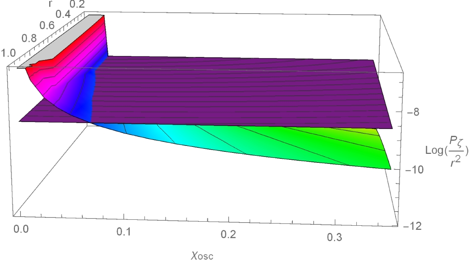
Figure 2. (color online) Plot of power spectrum: Using the COBE normalization [30], we set
$ H_I = 3.0\times 10^{-5} $ and find that$ A_s = 2.1\times 10^{-9} $ ; this corresponds to the purple plate in the figure, where$r = r_{\rm decay}$ .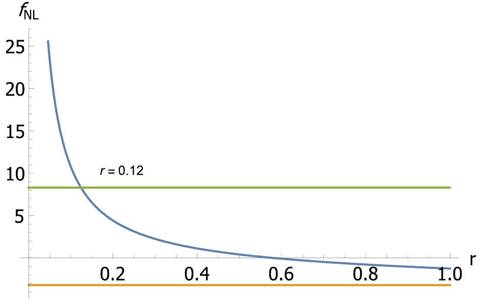
Figure 3. (color online) Plot of
$ f_{NL} $ : From the Planck Collaboration constraints on$ f_{NL} $ found in [19], we show the upper and lower bounds of$ f_{NL} $ . We find that the lower bound of$ r_{\rm decay}\approx 0.12 $ .Here, we provide a simple analysis of the curvaton decay. It can be explicitly seen that the curvaton mechanism is realized during the preheating process; meanwhile, the main contribution to the curvaton's potential is its direct coupling to the inflationary potential. Hence, the decay of the curvaton will be practically complete after preheating (i.e., the exponential potential becomes negligible compared to the coupling potential). Moreover, the generation of SM particles mainly occurs via the inflaton decay because the inflaton energy density is dominant before preheating. Thus, we conclude that particles are only produced via the inflaton decay. In terms of the preconditions of the curvaton's decay, its effective mass should exceed the mass of the target particle. For instance, the Higgs particle's mass is 125 GeV (of order
$ 10^{-12} $ in Planck units); thus, the effective mass of the curvaton should exceed this. However, this process does not occur because the effective mass of the curvaton is$m_\chi = \dfrac{{\rm d}^2V(\chi)}{{\rm d}\chi^2} =$ (of order$ 10^{-120} $ ), where$ V(\chi) = \lambda_0\exp\bigg(-\lambda_1\dfrac{\chi}{M_P}\bigg) $ . The same discussions apply to fermions. Finally, a relic of the exponential potential will remain into the late Universe.In this section, we predicted the power spectrum and non-local non-Gaussianity of the curvaton under the framework of the
$ \delta N $ formalism; by taking the appropriate approximations for the calculation, our results are seen to be independent of the inflationary potential. From Fig. 2 and Fig. 3, the constraints of$r_{\rm decay}$ can be found (specifically, for its lower bound). Once the transferral of energy from the inflaton to curvaton has occured, the generation of curvature is a natural process. -
Currently, dark energy is considered responsible for the accelerated expansion of the Universe; however, its origins remain mysterious. Of the many proposed mechanisms, the cosmological constant is the simplest explanation of dark energy; it was first proposed by Einstein [41] and was discovered to be capable of functioning as dark energy by James Peebles
$ e.t.c $ [42].In our scenario, the dark energy is mimicked by the exponential curvaton potential in the action (Eq. (1)). This action indicates that the effective mass becomes very small when the inflationary field vanishes; this leaves only the exponential curvaton potential to dominate and play the role of cosmological constant. The Universe is currently in a dark epoch, being dominated by dark energy; thus, the curvaton field should have almost vanished through decay into other particles; in particular, the particles of the SM. From the lower bound of
$ \frac{\chi_*}{H_*} = 7.0\times 10^ 4 $ found in [43] and the good approximation that$ H_I = H_* = 3.0\times 10^{-5} $ in Planck units, one readily obtains that$ \chi_* = 2.1 $ . Then, we use Eq. (39) between$\chi_{\rm osc}$ and$ \chi_* $ ; this relation can approximated to$\chi_{\rm osc}\approx \chi_*\exp(-2g\Delta N)$ , where$ c\approx 3 $ is used and$ \Delta N $ denotes the variance of the e-folding number; that is,$ \Delta N > 60 $ . Here, we set$ \Delta N \approx 100 $ . Meanwhile,$ g_0 $ is approximately constrained as$ 0.01 $ from Fig. 1; this yields$\chi_{\rm osc}\approx \chi_*\exp(-2)\approx 0.28$ , which is expressed for the moment at which the curvaton field begins to oscillate, though it could be even smaller as a result of the decay and eventual vanishing of the curvaton. From another perspective, the extra parameter$ \lambda_1 $ is not determined by observation. Because of the smallness of$ \chi_{e} $ , which denotes the final value after decaying, we have considerable freedom to choose the range of$ \lambda_1 $ , only being required to maintain$ \lambda_1\dfrac{\chi_e}{M_p}\ll 1 $ ; thus, the exponential potential approaches a constant$ \lambda_0 $ . Then, we retain$ \lambda_0\approx 10^{-120} $ in Planck units. This potential naturally plays the role of a cosmological constant. Finally, the Universe enters the dark epoch. -
In this paper, we constructed a broad class of curvaton scenarios, in which the effective mass of the curvaton is running as a result of the coupling between the curvaton and inflaton. The effective mass of the curvaton was found proportional to the inflationary potential, as shown in the action (Eq. (1)). The advantages of this mechanism are as follows: (a) the spectral index of the curvaton only depends upon the e-folding number and coupling coefficient; thus, a large class of inflationary models are compatible with this mechanism. (b) Once the curvaton has been generated by preheating, we calculate the power spectrum and non-linear non-Gaussianity; by neglecting the contribution of the exponential curvaton potential, we demonstrate that these two observables are independent of the inflationary potential. (c) After the decay of the curvaton, the exponential curvaton potential will approach a constant value of the order of the cosmological constant, which may play the role of dark energy. Finally, we constructed a large class of curvaton scenarios; these are practically model-independent, only requiring that the slow-roll inflationary conditions are satisfied for the inflaton and curvaton. Using these advantages, we systematically investigate our curvaton mechanism.
At first, only one field (i.e., the inflaton field) was present at the very beginning of the Universe. Subsequently, energy was transferred from the inflaton to the curvaton via a preheating process. In Section 3, we demonstrated that this production includes the background field and quantum fluctuations of the curvaton, and that it can be divided into two cases: narrow resonance and broad resonance. For narrow resonance, using constraints from the number density of curvatons and the decay rate of inflatons (i.e., the energy transferred from the inflaton to curvaton), we conclude that the inflationary field is large (i.e., its initial value is much larger than its effective mass). For broad resonance, the lower bound of
$m_{\rm eff}^2 g_0\phi_0^2\geqslant \dfrac{2\lambda_{0}\lambda_{1}^{2}}{g_0}$ was given. After generating the curvaton, we calculated its power spectrum and local non-Gaussianity. Our results agree with the observational constraints in Figs. 2 and 3. Remarkably, we found these results to be independent of the inflationary potential; however, the effective mass of the curvaton was proportional to the inflationary potential. This leaves extensive freedom when constructing the inflationary term.Finally, as the curvaton decay proceeds, its field value becomes increasingly small. In Section 4, we discussed how the exponential potential approaches a constant
$ \lambda_0 $ that is comparable to the cosmological constant. Therefore, from a phenomenological perspective, this relic of the exponential potential could play the role of the cosmological constant.Here, we outline relevant future work. The curvaton field arising from the preheating process was first investigated within the framework of bounce cosmology [44]. Then, the same curvaton field was found to be induced by the preheating process around the nonsingular bounce [45]. These works differ from our curvaton scenario in terms of the coupling between the inflaton and curvaton: in our case, the
$ \chi $ field explicitly couples to the inflationary potential. Furthermore, our calculations of observables are independent of the inflationary potential. This suggests that our curvaton mechanism can be realized within the framework of a bounce universe. However, the nature of the inflaton remains mysterious. As Ref. [4] described, prior to a certain moment$ t_1 $ , the expectation value of the inflationary field is zero; that is,$ \langle\phi^2\rangle = 0 $ . As it approaches the phase transition,$ \langle\phi^2\rangle $ becomes non-vanishing; thus, the interaction between$ \chi $ and$ \phi $ is no longer non-zero, which might naturally generate the curvaton mass through symmetry breaking. Thus, we could consider the inflationary field as a Higgs field, in light of the conclusions presented in [16, 17]. In our curvaton scenario, we could construct the Higgs field to power inflation and the curvaton to generate curvature perturbations. Furthermore, the one-loop correction can be considered under the framework of finite-temperature field theory; in particular, the effects of temperature may be observable. In the near future, we might also use asymptotic safety to construct the inflationary term [46]; however, we are also interested in studying the dark matter constraint within the framework of brane worlds [47-50].LH is grateful to Ai-Chen Li and Hai-qing Zhang for their fruitful discussions and comments regarding this manuscript, and thankful for the hospitality of the Institute of Theoretical Physics in Beijing University of Technology and Beihang University when starting this project. LH is indebted to his Ph.D supervisor, Prof. Tomislav Prokopec, who helped with the calculations of the Appendix, and he is exceedingly thankful for the guidance and endless discussions he received during his entire PhD period.
-
Here, we report a method of calculating the spectrum of curvaton perturbations during inflation, using the simplest tree-level (linearized) approximation. On a fixed cosmological gravitational background, the curvaton dynamics are governed by Eq. (27), which is valid provided the curvaton can be regarded as a spectator field; that is, if its energy density is subdominant during inflation. Assuming this is true, and further assuming that the curvaton perturbations are small, one can linearize Eq. (27) around the background field values
$ \bar\chi_E(t) = \langle\hat \chi_E\rangle $ and$ \bar\phi_E(t) = \langle\hat \phi_E\rangle $ such that, upon a convenient rescaling and linearization, Eq. (27) simplifies to$ \tag{A1} \left(\partial_0^2-\nabla^2+a^2V_E''-\frac{a''}{a}\right)(a\delta \hat\chi_E) = 0 \,, $

where
$ \delta \hat\chi_E = \hat\chi_E-\langle\hat\chi_E\rangle $ ,$ V_E'' = \partial^2 V_E(\bar\chi_E,\bar\phi_E)/\partial^2 \bar\chi_E $ , and$a'' = {\rm d}^2a/{\rm d}\tau^2$ . Because the background (Eq. (26)) is invariant under spatial translations, it is natural to assume that the state respects the same symmetry. Thus, we can expand$ \delta \hat \chi_E(x) $ in terms of mode functions$ \chi_E(\tau,k) $ and$ \chi^*_E(\tau,k) $ , as follows:$\tag{A2} \delta \hat{\chi}_E(\tau,\vec x) = \int\frac{{\rm d}^{3}k}{(2\pi)^{3}}{\rm e}^{\imath \vec{k}\cdot \vec{x}} \left[\chi_E(\tau,k)\hat{a}(\vec{k}\,)+\chi_E^*(\tau,k)\hat{a}^\dagger(-\vec{k}\,)\right] \,, $

where
$ k = \|\vec{k}\| $ ;$ \hat{a}(\vec{k}\,) $ is the particle annihilation operator that annihilates the vacuum$ |\Omega\rangle $ (that is,$ \hat{a}(\vec{k})|\Omega\rangle = 0 $ ); and$ \hat{a}^+(\vec{k}\,) $ is the particle creation operator that creates one quantum of momentum$ \vec k $ . These operators obey$\tag{A3}\begin{split} [\hat a(\vec{k}\,),\hat a^+(\vec{k}'\,)] =& (2\pi)^{3}\delta^{3}(\vec{k}\!-\!\vec{k}'\,) \,,\\ [\hat a(\tau,\vec{k}\,),\hat a(\tau,\vec{k}'\,)] =& 0 \,,\\ [\hat a^+(\tau,\vec{k}\,),\hat a^+(\tau,\vec{k}'\,)] =& 0 \,. \end{split}$

From (A1), the mode function
$ \chi_E(\tau,k) $ can be seen to satisfy the following differential equation:$ \tag{A4} \left(\frac{{\rm d}^2}{{\rm d}\tau^2}+k^2 + a^2V_E''-\frac{a''}{a} \right)[a\chi_E(\tau,k)] = 0 \,. $

The last term in (A4) can be written as
$ \tag{A5} \frac{a''}{a} = {\cal H}_E^2\left(1+\frac{{\cal H}_E'}{{\cal H}_E^2}\right) = {\cal H}_E^2\left(2-\epsilon_1\right) , $

$ \tag{A6} \epsilon_1 = -\frac{\dot H_E}{H_E^2} = 1-\frac{{\cal H}_E'}{{\cal H}_E^2} $

is the principal slow-roll parameter. The conformal Hubble parameter
$ {\cal H}_E $ can be expressed in terms of the conformal time and a power series of slow roll parameters, as follows:$ \tag{A7} {\cal H}_E = -\frac{1}{\tau}\left[1+\epsilon_1+\epsilon_1(\epsilon_1+\epsilon_2)+{\cal O}(\epsilon_i^3)\right] \,. $

Considering these relations and computing to second order in slow-roll parameters, Eq. (A4) becomes
$ \tag{A8} \left(\frac{{\rm d}^2}{{\rm d}\tau^2}+k^2 -\frac{1}{\tau^2}\left[2\!+\!3\epsilon_1\!+\!4\epsilon_1(\epsilon_1\!+\!\epsilon_2) +\frac32 (1\!+\!2\epsilon_1\! )\eta_c+{\cal O}(\epsilon_i^3,\eta_c\epsilon_j^2)\right]\right)[a\chi_E(\tau,k)] = 0 \,, $

where we have introduced the principal curvaton slow-roll parameter
$ \eta_c $ and the secondary slow-roll parameter$ \epsilon_2 $ as$ \tag{A9} \eta_c = -\frac23\frac{V_E''}{H_E^2} \,,\qquad \epsilon_2 = \frac{\dot\epsilon_1}{\epsilon_1H} \,. $

Assuming that the term that multiplies
$ 1/\tau^2 $ in Eq. (A8) varies adiabatically in time, Eq. (A8) can be solved in terms of Hankel functions. The fundamental solutions are given by$ \tag{A10} \psi(\tau,k) = \frac{1}{a}\sqrt{\frac{-\pi\tau}{4}}H_\nu^{(1)}(-k\tau), \quad \psi^*(\tau,k) = \frac{1}{a}\sqrt{\frac{-\pi\tau}{4}}H_\nu^{(2)}(-k\tau) \,, $

where the Wronskian normalization is
$ \tag{A11} W[\psi(\tau,k),\psi^*(\tau,k)] = \frac{\imath}{a^2} \,, $

and the index reads
$ \tag{A12}\begin{split} \nu^2 =& \frac94+3\epsilon_1+\frac32\eta_c+\epsilon_1(4\epsilon_1\!+\!4\epsilon_2+3\eta_c) \;\Longrightarrow\; \nu\simeq \frac32 +\epsilon_1\\&+\frac{1}{2}\eta_c +\frac13\epsilon_1\left(3\epsilon_1+4\epsilon_2+3\eta_c\right) +{\cal O}(\epsilon_i^3,\eta_c\epsilon_i^2) \,. \end{split} $

The general mode, consistent with spatial homogeneity and isotropy, is then
$ \tag{A13} \chi_E(\tau,k) = \alpha(k) \psi(\tau,k)+\beta(k)\psi^*(\tau,k) \,,\quad |\alpha(k)|^2-|\beta(k)|^2 = 1 \,. $

A standard Bunch-Davies choice of vacuum entails that
$ \alpha(k) = 1 $ and$ \beta(k) = 0 $ , which is what we assume throughout this work.The corresponding power spectrum and spectral index are defined via
$ \tag{A14} P_{\chi_E}(\tau,k) = \frac{k^3}{2\pi^2}|\chi_E|^2 = P_{\chi_E*}\left(\frac{k}{k_*}\right)^{n_{\chi_E}} \,. $

By applying Eqs. (A13) and (A10) in Eq. (A14), one obtains
$\tag{A15} P_{\chi_E}(k,\tau) = \frac{1}{a^2}\frac{k^3|\tau|}{8\pi}|H_\nu^{(1)}(-k\tau)|^2 \,. $

We are particularly interested in super-Hubble scales, where
$ |k\tau|\ll 1 $ ; the Hankel functions of the first kind,$ \tag{A16} H_\nu^{(1)}(-k\tau) = \frac{1}{\sin(\pi\nu)}\left[{\rm e}^{{\rm i}\pi\nu}J_\nu(-k\tau)-\imath J_{-\nu}(-k\tau)\right] \; \; \; \; (|\arg[-k\tau]| < \pi) \, $

can be expanded as
$ \tag{A17} \begin{split} H_\nu^{(1)}(-k\tau) = & \frac{1}{\pi}\left[-{\rm e}^{{\rm i}\pi\nu}\Gamma(-\nu)\left(\frac{-k\tau}{2}\right)^\nu-\imath \Gamma(\nu)\left(\frac{-k\tau}{2}\right)^{-\nu}\right]\\ & +{\cal O}\left(|k\tau|^{\nu+2},|k\tau|^{-\nu+2}\right) \,. \end{split} $

Because
$ \nu > 0 $ , the second term of Eq. (A17) dominates and we obtain the curvaton power spectrum on super-Hubble scales, as follows:$ \tag{A18} P_{\chi_E}(\tau,k) = \frac{H_E^2\Gamma^2(\nu)}{\pi^3[1+\epsilon_1+\epsilon_1(\epsilon_1+\epsilon_2)]^2} \left[\frac{k[1+\epsilon_1+\epsilon_1(\epsilon_1+\epsilon_2)]}{2H_Ea}\right]^{n_\chi} \,, $

with
$ \nu $ given in Eq. (A12), which becomes$ \tag{A19} n_\chi = 3-2\nu = -2\epsilon_1-\eta_c -\frac23\epsilon_1\left(3\epsilon_1+4\epsilon_2+3\eta_c\right) +{\cal O}(\epsilon_i^3,\eta_c\epsilon_i^2), $

where we have used
$ -k\tau\approx k[1+\epsilon_1+\epsilon_1(\epsilon_1+\epsilon_2)]/(H_Ea) $ (see Eq. (A7)). From Eq. (A18), we can easily read off the spectrum amplitude$ P_{\chi_E*} $ . To linear order in the slow roll parameters, it reads$ \tag{A20} \begin{split} P_{\chi_E* }(t,k_*) = & \frac{H_E^2}{4\pi^2}\Big[1 - 2\epsilon_1 + \frac23(2\epsilon_1 + \eta_c)\psi(3/2)\Big] \\ & \times \exp\Big[ - n_\chi\Big(N+\ln\frac{2H_E(1 - \epsilon_1)}{k_*}\Big)\Big] \,, \end{split} $

where
$ \psi(3/2) = 2-\gamma_E-2\ln(2)\approx 0.0367 $ is the di-gamma function of$ 3/2 $ , and$ H^2\simeq H_0^2{\rm e}^{-2\epsilon_1N} $ . The amplitude$ P_{\chi_E* } $ can be seen to depend weakly on time. For example, for a red-tilted spectrum in which$ n_\chi<0 $ ,$ P_{\chi_E* } $ grows exponentially with the number of e-foldings$ N = \ln(a) $ ; for example, for$ n_\chi\simeq -0.04 $ and$ \epsilon_1 = 0.01 $ ,$ P_{\chi_E* } $ increases by approximately 2% per e-folding.
The running curvaton
- Received Date: 2020-03-24
- Available Online: 2020-08-01
Abstract: In this paper, we propose a homogeneous curvaton mechanism that operates during the preheating process and in which the effective mass is running (i.e., its potential consists of a coupling term and an exponential term whose contribution is subdominant thereto). This mechanism can be classified into either narrow resonance or broad resonance cases, with the spectral index of the curvaton consituting the deciding criteria. The inflationary potential is that of chaotic inflation (i.e., a quadratic potential), which could result in a smooth transition into the preheating process. The entropy perturbations are converted into curvature perturbations, which we validate using the


 DownLoad: