


 Abstract
 HTML
HTML Reference
 Related
 PDF
PDF


-
One of the most important developments in AdS/CFT correspondence in the past few years is the discovery of the Ryu-Takayanagi (RT) entanglement entropy formula [1]. This formula states that the entanglement entropy of a subregion A of a
$ d+1 $ -dimensional CFT on the boundary of a$ d+2 $ -dimensional AdS is proportional to the area of a certain codimension-two extreme surface in the bulk:${S_A} = \frac{{{\rm{area}}(m(A))}}{{4{G_N}}},$

(1) where
$ m(A) $ is the minimal bulk surface in AdS time slice, which is homologous to A, i.e.,$ m(A)\sim A $ . This formula connects two important concepts in different fields and suggests some deep relations between quantum gravity and quantum information. Recent progress clearly shows that the RT formula plays a central role in understanding the emergence of space-time.When exploring the conceptual implications of the RT formula, however, Freedman and Headrick in Ref. [2] first noticed some subtleties of the formula. For example, there is a strangely discontinuous transition of the bulk minimal surface under continuous deformations of A. To remove these subtleties, the authors invoked the notion of “flow”, which is defined as a divergenceless norm-bounded vector. Employing the max flow-min cut (MF/MC) principle, this “flow” interpretation of the RT formula becomes more reasonable, because the discontinuous jump disappears, and there is a more transparent information-theoretic meaning of the entanglement entropy properties. In the construction of the flow picture of the RT formula, the MF/MC theorem plays a central role. It roughly states that in some idealized limit, the transport capacity of a classical network is a measure of what needs to be cut to entirely sever the network.
This picture, however, is built on the classical theory of the network. Recent progress on holography and quantum information theory implies that the quantum plays an important role in the studies of space-time. For example, the TN/AdS correspondence (MERA/AdS, quantum error correction/AdS), complexity/action correspondence, etc. A more reasonable picture must be replaced by a quantum flow network, which is a tensor network, as describe below. In this sense, the above “flow” picture of the RT formula is a semi-classical approximation of some unknown quantum (and fundamental) formulations.
Thus, we employ a tensor network description of quantum physics. A recent study on entanglement in strongly coupled many-body systems developed a set of real-space renormalization group methods, such as the tensor network state representation [3, 4]. In the past few years, this has been extensively studied in statistical physics and condensed matter physics. A tensor network description of wavefunctions of a quantum many-body system has the advantage to tremendously reduce the number of parameters (from exponential to polynomial) needed in the computation. This makes it a highly efficient representation of the wavefunction of the system. Furthermore, the tensor network representation provides an easy way to visualize the entanglement structure, and the area law of the entanglement entropy is inherent in the network. The more attractive property arises from connections between the tensor network and AdS/CFT correspondence①, which was first pointed out by Swingle in Ref. [5]. In this study, the author noticed that the renormalization direction along the graph can be viewed as an emergent (discrete) radial dimension of the AdS space. From this perspective, the holography stems from physics at different energy scales, and the AdS geometry can emerge from QFTs [6]. With regard to the holographic entanglement entropy, the tensor network-based RT formula can be interpreted as sum of all d.o.f of neighbor sites from UV to IR.
A natural question arises from these considerations: what is the “flow” picture of the tensor-network based RT formula? In this study, we mainly focus on the answer to this question. The solution requires the quantum MF/MC (QMF/QMC) theorem, which was recently presented in Refs. [7, 8]. This theorem, which is a quantum analogy of the MF/MC for tensor networks, states that the quantum max-flow of a tensor network is no larger than the quantum min-cut of the network. Particularly, for some tensor networks such as MERA①, the quantum max-flow is equal to the quantum min-cut, in the large central charge c limit. Based on this theorem and information-theoretic considerations, we define a new variable
$ \rho $ , which can be interpreted as the density of the tensor networks under question. The physical integral of$ \rho $ over a region can be viewed as the source (or sink) of the tensor networks, and it plays a significant role in the flow description of the RT formula. We show that it determines the structure of the tensor network on the basis of a fixed Lorentzian manifold$({\cal M},g)$ . More precisely,$ {\rm d}V_{\rm network} = \rho (x)\sqrt{g}{\rm d}V $ of this tensor network. When$ \rho(x) = $ constant, it reduces to the kinematic space of an$ {\rm AdS}_3 $ time-slice [9, 10], and the corresponding tensor network is MERA. Further, from the informaton viewpoint,$ \rho(x = (i,j)) $ is the density of compression or decompression of quantum bits through reducing or expanding the dimensions of Hilbert space. It encodes to what extent information is shared between two sites i and j. Hence,$ \rho(x) $ provides the local contributions of these sites to the total conditional mutual information.This paper is organized as follows. In Section 2, we first provide a brief review of Freedman-Headrick’s proposal of bit threads and holography, followed by a brief introduction to the QMF/QMC theorem. To determine the relation between the QMF/QMC theorem and the RT formula for the MERA tensor network, we also review the MERA in kinematic space. In Section 3, we briefly import our main results from informational points of view. In Section 4, we propose our “flow” language of a tensor network with the help of the QMF/QMC theorem. Section 5 presents an information-theoretic interpretation of the MERA, with particular interests in the information-theoretic meaning of the isometry. Several physical key points of the picture are also discussed in this section. In last section, we draw our main conclusions and provide the discussions.
-
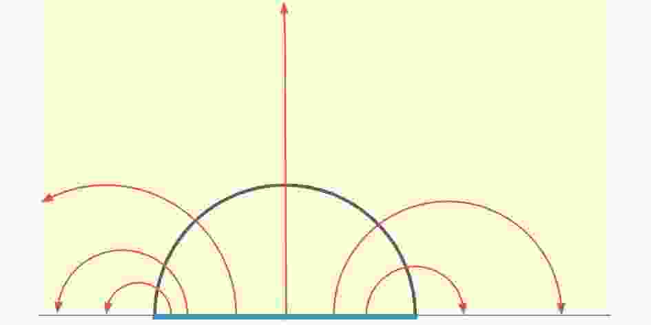
The RT formula (1) can be reinterpreted as a “max-flow” from the max-flow/min-cut (MF/MC) theorem in Riemannian geometry first explored in Ref. [2]. This can be viewed as calibrations to the Ryu-Takayanagi minimal surfaces [11]. To elaborate on this point, we define a divergenceless vector field v as a “flow” satisfying the following two properties [2] (as shown in Fig. 1):
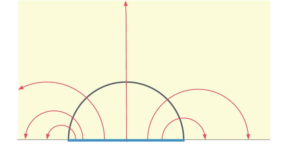
Figure 1. (color online) Max-flow min-cut picture of a subregion. Red line depicts the bit threads with maximal density on a minimal surface (black curve).
$|v| \leqslant C,$

(2) ${\nabla _\mu }{v^\mu } = 0,$

(3) where C is a positive constant. Then, the flux of v through an oriented manifold surface
$ m \sim A $ can be defined as an integral:$\int_{m(A)} v : = \int_{m(A)} {\sqrt h } {n_\mu }{v^\mu },$

(4) where h is the determinant of the induced metric on m, and
$ n_\mu $ is the unit normal vector. The maximal flux should be bounded by a bottleneck$\int_A v = \int_{m(A)} v \leqslant C\int_{m(A)} {\sqrt h } = C{\rm{area}}(m).$

(5) This inequality is saturated by C, where
$ n_\mu v^\mu = C $ holds. This indicates that a flow reaches its maximum if and only if$ n_\mu v^\mu = C $ , and the maximal flux is equal to the minimal area multiplying a constant:$\mathop {\max }\limits_v \int_A v = C\mathop {\min }\limits_{m \sim A} {\rm{area}}(m).$

(6) Two extensions of the theorem must be introduced. First, when we continuously change A, the maximal flow
$ v(A) $ likewise varies continuously. Second, considering two disjoint regions A and B of the boundary, we generally cannot find a flow that maximizes the flux through A and B simultaneously, i.e.$\begin{split} \int_A v + \int_B v =& \int_{AB} v \leqslant C{\rm{area}}(m(AB))\\& < C{\rm{area}}(m(A)) + C{\rm{area}}(m(B)). \end{split}$

(7) We call this the “nesting” property.
Returning to holography, the minimal area can be replaced with the maximal flow, and the RT formula can be rewritten in the following manner:
$S(A) = \mathop {\max }\limits_v \int_A v ,$

(8) where
$ C = 1/(4G_N) $ . A magnetic field can be visualized as field lines. Similarly, these flow lines v can be regarded as oriented “bit threads” from boundary to bulk. The upper bound$ 1/(4G_N) $ of flow can be interpreted as follows: the bit threads cannot be tighter than one per four Planck areas in$ 1/N $ effects. Then, a thread that emanates from the boundary region A should be viewed as one independent bit of information originating from A. From this point of view, the maximal number of independent information bits is the entanglement entropy$ S(A) $ .From this “flow” language, we can also obtain the conditional entropy and mutual information. Let
$ v(A;B) $ denote the flow that not only maximizes the flux through A, but also maximizes the flux through AB, i.e.$ v(A) $ or$ v(A,B) $ . Then, the conditional entropy$ H(A|B): = S(AB)- S(B) $ can be rewritten as an expression in terms of flows [2]. Considering two regions case, the conditional entropy can be written as$\begin{split}H(A|B) =& \int_{AB} v (B;A) - \int_B v (B;A) \\=& \int_A v (B;A). \end{split}$

(9) Simultaneously, the flux through A reaches its minima. Hence, we can express the mutual information
$ I(A:C) : = S(A)-H(A|C) $ . Without loss of generality, we can choose the entropy of A:$ \int_A v(A;C) $ , then$ I(A:C) $ can be rewritten as$\begin{split}I(A:B) =& \int_A v (A;B) - \int_A v (B;A)\\=& \int_A {(v(} A;B) - v(B;A)).\end{split}$

(10) This is the flux that can be shifted between A and C. Similarly, in the three regions case, we can express the conditional mutual information
$ I(A:C|B) : =S(AB)+$ $ S(BC)-S(ABC)-S(B) = H(A|C)-H(A|BC) $ . Without loss of generality, we can choose$ H(A|B) = \int_A v(B,A;C) $ and$ H(A|BC) = \int_A v(B,C;A) $ . In this way,$ I(A:C|B) $ can be expressed as:$\begin{split}I(A:C|B) =& \int_A v (B,A;C) - \int_A v (B,C;A)\\=& \int_A {(v(} B,A;C) - v(B,C;A)).\end{split}$

(11) -
The quantum max-flow min-cut (QMF/QMC) conjecture was first presented in Ref. [7]. Subsequently, in Ref. [8], Cui et al. showed that this conjecture dose not generally hold, except for some given conditions. There are two versions of this conjecture, and we first review the first version.
The tensor network can be regarded as a graph
$ G(\tilde V,E) $ , which is unoriented with a set of inputs S and a set of outputs T.$ \tilde V $ is a disjoint partition$ \tilde V = S \bigcup T \bigcup V $ . E is a set of edges with a capacity function$ a: E\to \mathbb N, $ $e \mapsto a_e $ . In the tensor network, each edge e is associated with a Hilbert space$ \mathbb C^{a_e} $ , and the edges capacity corresponds to dimensions of the Hilbert space. Inputs S and outputs T can be thought of as some open edges with open ends for convenience. V is a set of vertices, such that for each vertex v, there are$ d_v $ edges$ e(v,1), e(v,2), \cdots , e(v,d_v) $ incident to v. Associating a tensor to every vertex$ v\mapsto {\cal T}_v \in {\cal I}^v: = \bigotimes_{i = 1}^{d_V} \mathbb C^{a_e} $ thus sends a graph G to a tensor network,$ G \mapsto N(G,a;{\cal T}) $ (as an example, please see Fig. 2 provides an example). After fixing basis of the Hilbert space of the open edges, we can determine a state$ |\alpha(G,a;{\cal T})\rangle \in V_S \bigotimes V_T $ , which is given by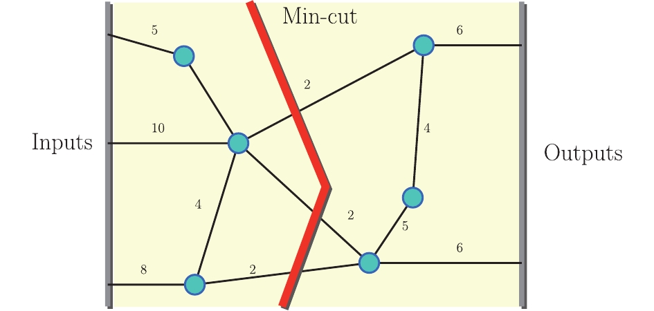
Figure 2. (color online) A tensor network with three inputs and two outputs. Blue balls depict vertices associating tensors, and black lines depict edges associating different Hilbert dimensions. The red line illustrates the minimal cut of this network.
$\begin{split} |\alpha (G,a;{\cal T})\rangle : =& {\sum\limits_{\begin{array}{*{20}{c}} {{{i_1}, \cdots ,{i_{\left| S \right|}}}}\\[-5pt] {{{j_1}, \cdots ,{j_{\left| T \right|}}}} \end{array}} {{C_{{i_1}, \cdots ,{i_{|S|}},{j_1}, \cdots ,{j_{|T|}}}}} }\\ &{ \times |{i_1}, \cdots ,{i_{|S|}}{\rangle _S}|{j_1}, \cdots ,{j_{|T|}}{\rangle _T},} \end{split}$

(12) where
$ V_S: = \bigotimes_{u\in S}\mathbb C^{a_{e(u)}} $ and$ V_T: = \bigotimes_{u\in T}\mathbb C^{a_{e(u)}} $ . With these, we can define a quantum max flow and min cut.Primarily, the definition of “cut” must be stated. If there is a partition
$ \tilde V = \bar S \bigcup \bar T $ , such that$ S\subset\bar S, T\subset\bar T $ , then a cut A is a set that$ A = \{(u,v) \subset E:u\in \bar S,v\in \bar T\} $ . Intuitively, removing the edges in C will lead to a disconnect in the path from S to T.Definition 1 (Quantum min-cut). The quantum min-cut
$ {\rm QMC}(G,a) $ is the minimum value of the product of capacities over all edge cut sets, i.e.${\rm QMC}(G,a): = \mathop {\min }\limits_A \;\prod\limits_{e \in C} {{a_e}} .$

(13) There is a linear map
$ \beta(G,a;{\cal T}) \in V_S^* \!\bigotimes\! $ $V_T\!\! =\!\! Hom(V_S, V_T) $ from inputs to outputs:$ V_S \mapsto V_T $ acting on the inputs state:$\begin{split} \beta (G,a;{\cal T})|{i_1}, \cdots ,{i_{|S|}}{\rangle _S}: =& {\sum\limits_{{j_1}, \cdots ,{j_{|T|}}} {{C_{{i_1}, \cdots ,{i_{|S|}},{j_1}, \cdots ,{j_{|T|}}}}} }\\ &{ \times |{j_1}, \cdots ,{j_{|T|}}{\rangle _T}.} \end{split}$

(14) Evidently, in this basis the matrix C is exactly
$ \beta (G,a;{\cal T}) $ . Then, one can define the quantum max-flow as follows:Definition 2 (Quantum max-flow). Across all tensor assignments, there is a maximal value of the rank of map
$ \beta(G,a;{\cal T}) $ , which we define as the quantum max-flow:${\rm QMF}(G,a): = \mathop {\max }\limits_{\cal T} \;{\rm rank}(\beta (G,a;{\cal T})).$

(15) Cui et al. [8] stated that
$ {\rm QMF}(G,a) $ is generally not equal to$ {\rm QMC}(G,a) $ . In fact,$ {\rm QMF}(G,a) $ is consistently smaller than$ {\rm QMC}(G,a) $ in a given finite graph G:$ {\rm QMF}(G,a)\leqslant {\rm QMC}(G,a) $ . The equality holds in a special case, which can be considered as a weak QMF/QMC:Theorem 1 (Quantum max-flow min-cut theorem). For a given graph
$ G(\tilde V,E) $ , if the capacity a of each edge is a power of d, where$ d>0 $ is an integer, then$ {\rm QMF}(G,a) = {\rm QMC}(G,a). $

(16) Here, we turn to the entanglement entropy between inputs and outputs of the tensor network and see its relation with the QMF and QMC. The Hilbert space of pure states (13) is
$ {\cal H} = V_S \bigotimes V_T $ , and we can obtain the reduced density matrix of$ |\alpha(G,a;{\cal T})\rangle $ on S by tracing T:$\begin{split} {{\rho _S}\left( {\frac{{|\alpha (G,a;{\cal T})\rangle }}{{\sqrt {{\rm Tr}(C{C^\dagger })} }}} \right)} =& {{\rm Tr}_T}\;|\alpha (G,a;{\cal T})\rangle \langle \alpha (G,a;{\cal T})|\\ =&{ \frac{{C{C^\dagger }}}{{{\rm Tr}(C{C^\dagger })}},} \end{split}$

(17) where
$ {\rm Tr}(CC^\dagger) = \sum_{i_1,\cdots,i_{|S|},j_1,\cdots,j_{|T|}}|C_{i_1,\cdots,i_{|S|},j_1,\cdots,j_{|T|}}|^2 $ , and$ \frac{|\alpha(G,a;{\cal T})\rangle}{\sqrt{{\rm Tr}\ CC^\dagger}} $ is a normalized state. We already know the von Neumann entropy is$ S(\rho): = -{\rm Tr}\ (\rho\log \rho) $ . Hence, we define an entanglement entropy between S and T:$\begin{split} EE(G,a;{\cal T}): =& S\left( {\frac{{C{C^\dagger }}}{{{\rm Tr}(C{C^\dagger })}}} \right)\\ =& - \frac{{{\rm Tr}(C{C^\dagger }\log (C{C^\dagger }))}}{{{\rm Tr}(C{C^\dagger })}} + \log ({\rm Tr}(C{C^\dagger })). \end{split}$

(18) Letting
$ MEE(G,a) $ denote the maximal of$ EE(G,a) $ over all$ {\cal T}'s $ , we can prove that in general,$ MEE(G,a) \leqslant $ $ \log {\rm QMF}(G,a) \leqslant \log {\rm QMC}(G,a) $ . The equality holds when we consider the same case as Theorem 1, i.e.Theorem 2. For a given graph
$ G(\tilde V,E) $ , if the capacity a of each edge is a power of d, where$ d>0 $ is an integer, then$MEE(G,a) = \log {\rm QMC}(G,a) = \log {\rm QMF}(G,a).$

(19) The second version of the QMF/QMC conjecture is more restricted. The vertices of the same type must be assigned the same tensor. More specifically, we place an ordering O to the ends of the edges incident to each vertex and define a valence type
$ B_v $ of a vertex v to be the sequence$ (a_{e(v,1)},..., a_{e(v,d_v)}) $ , where$ a_{e(v,d_v)} $ is the dimension of the Hilbert space of edge$ e(v,d_v) $ . We denote$ {\cal B}(G,a,O) $ as the set of valence type of vertices of graph G. The vertices with the same valence type must be assigned the same tensor$ {\cal T} = \{{\cal T}_B:B\in{\cal B}(G,a,O)\} $ .From above, we obtain a linear map, which is denoted by
$ \beta(G,a,O;{\cal T}) $ in$ Hom(V_S,V_T) $ . The definition of the quantum max-flow$ {\rm QMF}(G,a,O) $ for this second version is the maximum rank of$ \beta(G,a,O;{\cal T}) $ , similar to the first version. The difference is as follows: Conditions stated in Theorem 1 are insufficient to guarantee the equality${\rm QMF} = $ $ {\rm QMC} $ , even when the Hilbert space dimension is same in each edge in the graph. The restriction of the tensor, or the quantum gate of the circuit is more nontrivial than the first version of QMF/QMC. The tensors of MERA network are restricted, and the second version of QMF/QMC is more suitable for our discussion. We still need some additional conditions, and we discuss this in the following. -
For convenience, we provide a brief review on the kinematic space that was firstly formulated in Refs. [9, 10]. Given a hyperbolic plane
$ \mathbb H^2 $ , which is a time slice of pure$ {\rm AdS}_3 $ space-time:${\rm d}{s^2} = {\rm d}{\rho ^2} + {\sinh ^2}\rho {\rm d}{\tilde \theta ^2}.$

(20) The equation of a space-like geodesic that anchors on boundary points is:
$\tanh \rho \cos (\tilde \theta - \theta ) = \cos \alpha ,$

(21) where
$ (\theta,\alpha) $ are parameters that label a oriented geodesic, as shown in Fig. 3. The space of all these geodesics$ (\theta,\alpha) $ forms a two-dimensional manifold, which we refer to as the kinematic space. A geodesic can be described by a point$ (\theta,\alpha) $ in the kinematic space. Crofton's formula in$ \mathbb H^2 $ states that the length of a curve$ \gamma $ can be measured by the number of geodesics that intersect it, i.e.,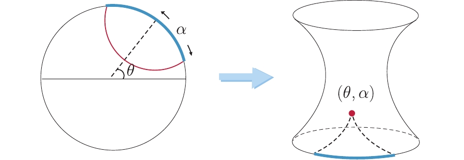
Figure 3. (color online) Space-like geodesic on AdS3 timeslice mapped to a point
$ (\theta,\alpha) $ in kinematic space.${\rm length\;of}\;\gamma = \frac{1}{4}\int_K n (g,\gamma ){\cal D}g,$

(22) where
$ n(g,\gamma) $ is the number of geodesics intersect$ \gamma $ , and$ {\cal D} g $ is the measure on the kinematic space${\cal D}g = \frac{{{\partial ^2}S(u,v)}}{{\partial u\partial v}}{\rm d}u{\rm d}v.$

(23) If the curve is a geodesic with two ends u and v anchoring on the boundary, then
$ S(u,v) $ is the length of the geodesic . We used a light-cone coordinate on the kinematic space,$u = \theta - \alpha, \;\;\;\;\;\;v = \theta + \alpha .$

(24) Eq. (23) also denotes the line element of the kinematic space multiplied by some coefficient
${\rm d}s_{\rm kinematic}^2 \sim \frac{{{\partial ^2}{S_{\rm ent}}(u,v)}}{{\partial u\partial v}}{\rm d}u{\rm d}v,$

(25) where we have replaced S by
$ S_{\rm ent} $ (the entanglement entropy) because of the RT formula. Therefore, the entanglement entropy can be represented by a volume in kinematic space,$\begin{split} {S_{\rm ent}} =& \frac{{\rm length\;of\;\gamma }}{{4G}}\\ =& \frac{1}{4}\int_K n (g,\gamma )\frac{{{\partial ^2}{S_{\rm ent}}(u,v)}}{{\partial u\partial v}}{\rm d}u{\rm d}v. \end{split}$

(26) Czech et al. [9] argued, considering the auxiliary causal structure of the MERA, it is the vacuum kinematic space instead of the
$ {\rm AdS}_3 $ time slice that should be viewed as the corresponding geometry of the MERA. Thus, the kinematic space becomes an intermediary in the AdS/CFT.One of the key points of this argument is the casual structure of the MERA. This makes it more natural to match such a network with a Lorentzian manifold, as first mentioned in Ref. [12]. In the following, we consider an exclusive causal cone for part of lattices. Boundary of this causal cone is called as causal cut of the MERA network as shown by the red line in Fig. 4(a). The method to calculate the entanglement entropy – given a holographic interest in MERA in Ref. [5] – involves simply counting the number of edges cut by the causal cut in this network, with each edge assigning a weight
$ \log\chi $ , where$ \chi $ is the Hilbert dimension of edges. In the same footing, we may also calculate the conditional mutual information by counting the number of edges. Recall that conditional mutual information is defined as follows:
Figure 4. (color online) (a) Causal cut of MERA tensor network. (b) Conditional mutual information
$ I(A:C|B) $ on boundary can be regarded as the volume of a causal domain in kinematic space.$I(A:C|B) = S(AB) + S(BC) - S(ABC) - S(B).$

(27) This means that the conditional mutual information can be obtained by counting the number of edges, which is the net reduction of edges through a causal diamond from the bottom up, as shown in Fig. 4(b). This is arguably the same as counting the number of isometries living in this diamond, as every isometry has two input edges and only one output edge from bottom up. Hence, each isometry soaks up an edge such that counting the number is equalent to counting the decrease in the number of edges. This indicates that the conditional mutual information is proportional to the number of isometries in the causal diamond and to the volume of this diamond, which is easily found by Eq. (25).
Based on these observations, connections can be built between conditional mutual information and the volume in kinematic space. Czech et al. [9] adopted conditional mutual information as a definition of volume in the MERA,
${\cal D}({\rm isometries}) = I(A:C|B).$

(28) This formula evaluates the volume after compressing the state living on its past edges. In this vacuum MERA, the ‘density of compression’ is proportional to the isometry number. More explicitly, the metric of a discrete tensor network is given by
$\begin{split} {\rm d}{s_{\rm network}} =& I(\Delta u,\Delta v|B)\\ &\xrightarrow{{\rm MERA}} (\# \;{\rm of\;isometries})\Delta u\Delta v, \end{split}$

(29) which is the metric of kinematic space, as well as the volume element in kinematic space.
-
As stated in the previous section, we prefer to treat MERA as a discrete kinematic space rather than the original slice of the AdS space. This statement is based on the following two advantages:
$ {\rm (a)} $ they share the same causal structure, and$ {\rm (b)} $ regarding entanglement as a “flux” through the causal cut, which is equivalent to counting the number of lines on the causal cut, has a more natural interpretation in kinematic space [9]. Consequently, bit threads in the AdS time slice should have an information-theoretic interpretation on kinematic space. To see this, we first recall flows in the AdS time slice. A flow v is a vector field, and we can define a set of integral curves of v, whose transverse density equals$ |v| $ . Each flow line, the so-called “bit threads”, is an oriented thread connecting two different points on the boundary. For example, given a time slice of AdS, we can split the boundary into two parts A and$ A^c $ , such that the information (flow) shared between A and$ A^c $ is$I(A:{A^c}) = 2S(A).$

(30) A thread between A and
$ A^c $ connects two points on A and$ A^c $ , one of which is the start point of the thread (belongs to A), whereas the other is the end point (belonging to$ A^c $ ). These two end points can be mapped to a point in the kinematic space, which is denoted by$ (u, v) $ . We therefore obtain a picture between the original and kinematic spaces, as shown in Fig. 5.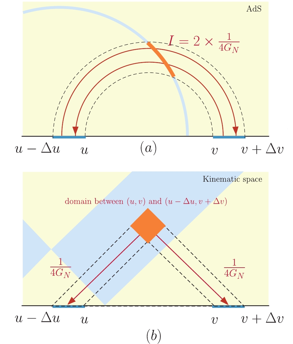
Figure 5. (color online) Conditional mutual information between
$ [u-{\rm d}u,u] $ and$ [v,v+{\rm d}v] $ , located in minimal surface can be interpreted as$ 2\times 1/4G_N $ decompressed information in kinematic space.In the previous section, we mentioned that one of the important properties of the bit threads is
$ |v|\leqslant 1/(4G_N) $ , which means that one cannot contain more than$ 1/(4G_N) $ information in the unit area. The flow density is saturated at the minimal surface$ m(A) $ , i.e.,$ |v| = 1/(4G_N) $ . This implies that we have$ 1/(4G_N) $ entanglement flow per unit area on the surface. From Eq. (30), we can assume that A and$ A^c $ share$ 2 \times 1/(4G_N) $ bits of information per unit area of the minimal surface, or equivalently,$ [u-\Delta u, u] $ and$ [v, v+\Delta v] $ on the boundary share$ 2\times1/(4G_N) $ bits of information. Mapping this “area” (which actually is a geodesic length in 2D) to the kinematic space yields a “volume” (an area in 2D) of some region, as shown in Fig. 5. This implies that$ 2 \times 1/(4G_N) $ bits of information in a unit area of the minimal surface correspond to$ 2 \times 1/(4G_N) $ bits of information in$ \Delta u\Delta v $ in the kinematic space (we set the radius of kinematic space to one). Regarding these partial contributions to the total$ I(A:A^c) $ , the relation between AdS and kinematic space is given by Fig. 6.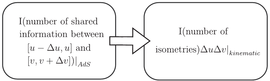
Figure 6. Relation between AdS and kinematic space.
This can be also seen from the causal structure perspective. The shared information between
$ [u-\Delta u,u] $ and$ [v, v+\Delta v] $ can be naively regarded as non-intersecting geodesics included in the tube$ ([u-\Delta u,u], [v, v+\Delta v]) $ in AdS [13], which are time-like between$ [u,v] $ and$ [u-\Delta u, v+\Delta v] $ . In kinematic space, these are isometries in a causal diamond between$ (u,v) $ and$ (u-\Delta u, v+\Delta v) $ , which, as expected, is the region where the conditional mutual information$ I([u,u-\Delta u]: [v,v+\Delta v]|[u,v]) $ is calculated.$ I([u,u-\Delta u]: [v,v+\Delta v]|[u,v]) $ , as a part of the total$ I(A:A^c) $ , is only related to the degrees of freedom between$ [u-\Delta u,u] $ and$ [v,v+\Delta v] $ . Therefore, we must introduce a local quantity associated with the isometries of the MERA in accordance with the above discussion.The above analysis strongly suggests to view the isometries as “sources” (or “sinks”) of information. Indeed, if we deem the information flow
$ 1/4G_N $ from top to bottom in the MERA through isometries, then these isometries decompress the bits. The decompression result is$ 2\times 1/(4G_N) $ , which is the conditional mutual information between$ [u-\Delta u, u] $ and$ [v, v+\Delta v] $ . The isometries play roles in sharing the information in these two intervals on the boundary, as shown in Fig. 5. Hence, isometries provide a local “density of compression (or decompression)” of the network, and such s MERA network can be regarded as an iterative compression algorithm, which maps the density matrix of a interval to a compressed state on the causal cut. The entangler also plays a key role but not important for our discussion and can be neglected [14]②.In this study, we attempt to further investigate the holography of tensor network from a different perspective: the QMF/QMC theorem. We discuss the quantum version of the network, which is different from the classical one of Headrick-Freedman. We attempt to set up a holography picture of the quantum network and study some general properties between the tensor network and space-time. The main results of this work are listed in the following:
1) For a quantum network, we introduce a density
$ \rho(x) $ to describe the QMF of a general tensor network. We focus on the MERA, which has some important properties (such as symmetry) for holography. We find from the QMF = QMC case that each edge has the same entanglement flow (assuming all edges have the same Hilbert dimension), and hence if there is isometry in the tensor network, the source (or sink) has to be introduced to preserve conservation of entanglement flow. Therefore, the quantum bit threads are studied in kinematic space, and we extend the picture of Czech et al. by introducing$ \rho $ .2) We realize that in MERA, the density
$ \rho $ encodes the local contributions of each degree of freedom to the total conditional mutual information between two intervals on the boundary. This is similar to the so-called entanglement contour recently studied in holography [15, 16]. We find that the definition of$ \rho $ meets some requirements similarly to the contour.3) We argue that in the MERA tensor network, which has the same type isometry everywhere, the “classical” limit QMF = QMC is equivalent to the classical limit of emerged space-time. This is the large central charge limit of the tensor network dual to classical gravity, which lacks discussion in other articles.
-
In this subsection, we consider the QMF=QMC case. Under this condition, the tensor between a causal cut and boundary is an isometric tensor, defined in Ref. [17]. We set the causal cut as the inputs S of the network and the corresponding boundary region as the outputs T of the network. Identifying
$ V_S^* $ with$ V_S $ by using the chosen basis in$ V_S $ , one can determine a state$ \alpha(G,a;{\cal T}) $ . We denote the basis of$ V_S, V_T $ as$ {|i\rangle_S},{|j\rangle_T} $ , respectively, and let matrix of$ \beta(G,a;{\cal T}) $ be C on this basis. Hence, we obtain$\alpha \left( {G,a;{\cal T}} \right) = \sum\limits_{i,j} {{C_{ji}}} |j{\rangle _T}|i{\rangle _S}.$

(31) Thus,
$ \beta $ is a tensor that maps from the causal cut to the boundary:$\beta :\;\;|i{\rangle _S}\; \mapsto \;\sum\limits_j {{C_{ji}}} |j{\rangle _T}.$

(32) We assume that S is a minimal cut and
$ \dim(S)\leqslant\dim(T) $ . If the QMF/QMC conjecture holds in this tensor network QMF = QMC, then after an appropriate ordering of the basis elements in$ V_S $ and$ V_T $ , the map$ \beta $ assumes a simple form [8]:$ \left( \begin{array}{ccc|c} \begin{matrix} 1&\; \; &\; \; \\ \; \; &\ddots&\; \; \\ \; \; &\; \; &1\\ \hline \; \; &0&\; \; \\ \end{matrix} \end{array}\right). $

(33) Letting
$ M = {\rm QMC}(G,a) $ be the dimension of inputs, the upper block matrix becomes$ M\times M $ . So we have$\sum\limits_j {\beta _{i'j}^\dagger } {\beta _{ji}} = {\delta _{i'i}}.$

(34) Here,
$ \beta $ is the so-called isometric tensor. The difference lies in that the tensor mentioned in Ref. [17] is defined in a negative curvature space, whereas ours is in kinematic space, which is a positive curvature space. Such a tensor network has an important property: the RT formula holds$ S_{EE} = |S|\cdot\log \chi $ . After a bipartition of the network, this implies that the two parts of this network have maximal entanglement. ($ |S| $ is the number of cut legs and$ \chi $ is the Hilbert dimension of each edge). From Eq. (18), we know that the entanglement entropy is given by the tensor C(or$ \beta $ ), which is more related to QMF. If the QMF/QMC holds asymptotically, the second term in Eq. (18) will be leading, and the entropy is given by the QMC in Eq. (19). In this case, each edge through the bipartition cut has a maximal entropy flow$ \log \chi $ . In the following subsection, our model is considered in the QMF = QMC case, and further interpretations are provided in Section 5.2. -
We start by explaining a tensor network in terms of “flow” language, which is convenient for our discussion. Supposing there is a flow through a boundary, which can be denoted by
$ f^\mu $ . Its flux$ {\cal F} $ through a boundary region A is obtained by integration$ f^\mu $ over this region:${\cal F} = \int_A f \;: = \int_A {\sqrt {|h|} } {n_\mu }{f^\mu },$

(35) where h is the determinant of the induced metric on A (because of the IR divergence, we should choose an IR cut-off surface
$ A_{\epsilon} $ , but we still use A for simplicity). The addition is thus satisfied:$\int_A f + \int_B f = \int_{AB} f ,$

(36) Next, we consider a cut
$ C_A\sim A $ to be an oriented codimension-one submanifold in the network, which is homologous to A. As claimed in the last section, isometries in the tensor network may play a role of the source (or sink). Therefore, different from bit threads in the original AdS slice, generally$ \int_{A} f \neq \int_{C_A} f $ . Instead, one extra term that describes the contributions from tensors should be added$\int_{{C_A}} f = \int_A f + \int_{{D_A}} \rho ,$

(37) where
$ \int_{D_A} \rho : = \int_{D_A}\rho\sqrt {-g}{\rm d} \omega $ , and g is the determinant of the metric on this Lorentzian manifold.$ D_A $ is the region enclosed in$ A\bigcup C_A $ . From Eq. (37), we obtain$\begin{split} 0 =& - \int_{AB} f - \int_{BC} f + \int_{ABC} f + \int_B f \\ =& \int_{{D_{AB}}} \rho + \int_{{D_{BC}}} \rho - \int_{{D_{ABC}}} \rho - \int_{{D_B}} \rho \\ &+ \int_{{C_{AB}}} f + \int_{{C_{BC}}} f - \int_{{C_{ABC}}} f - \int_{{C_B}} f = \int_D \rho + \oint_{\partial D} f . \end{split}$

(38) where D is the region
$ D_{ABC}+D_B-D_{AB}-D_{BC} $ . That means that for an arbitrary region in a network, the Gaussian theorem is consistently valid.$ \rho $ can be viewed as a density of tensors and must satisfy the following two properties:$|\rho | \leqslant {\rho _M},$

(39) ${\nabla _\mu }{f^\mu } = - \rho ,$

(40) where
$ \rho_M $ is a positive constant. The first constraint implies finiteness of the density. The second term of the last equality in Eq. (38) is the flux and can be denoted by$ {\cal D} $ . Eq. (38) indicates that the flux$ {\cal D} $ of the region D can also be calculated by a volume integral instead of a surface integral${\cal D}: = \oint_{\partial D} f = - \int_D \rho .$

(41) This implies that a flow is incoming from the bottom of the casual diamond. Meanwhile, the constraint
$ |\rho| \le \rho_M $ implies that the flux is bounded by$\left| {\cal D} \right| \leqslant {\rho _M}\int_D {\sqrt {|g|} } {\rm d}\omega = {\rho _M}{V_D}.$

(42) Hence, what does the flux represent in this picture? It is more reasonable if we regard the flux
$ \int_{C_A} f $ as the logarithm of the rank of$ \beta(G,a;{\cal T}) $ ③. Thus, we have treated edges on A as inputs and edges on$ C_A $ as outputs, as shown in Fig. 7, and the flux is given by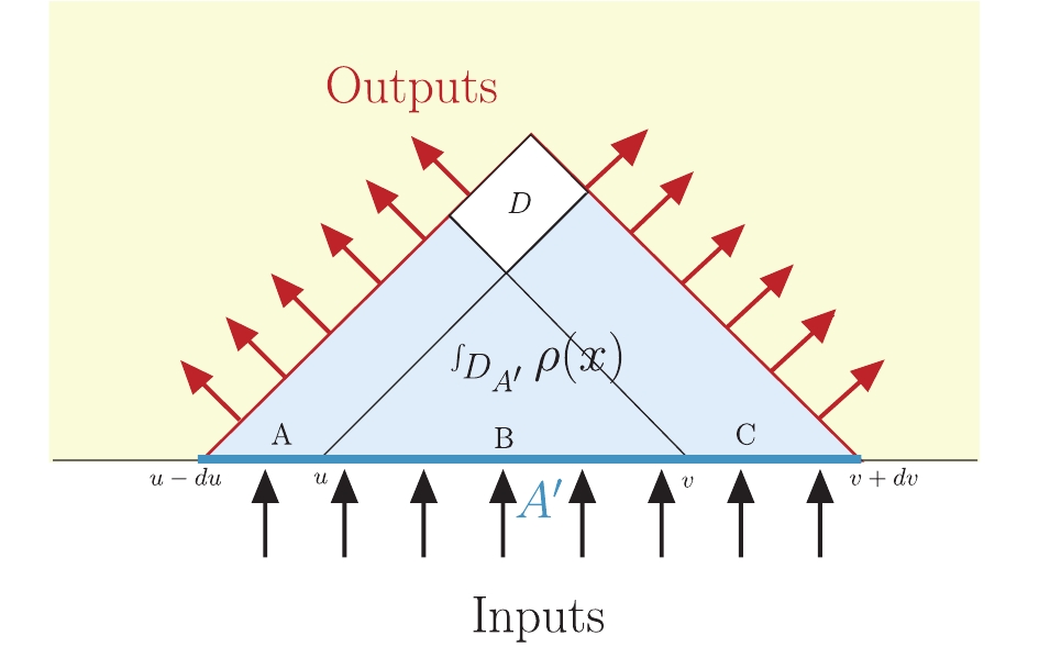
Figure 7. (color online) Cutoff legs as inputs
$ A' $ and causal cut legs as outputs$ C_{A'} $ . The blue triangle (including region D) is$ D_{A'} $ . For a general network, we can determine the causal cut of intervals A, B, C, AB, BC, and ABC. They determine a causal domain D (white region).$\int_{{C_A}} f \equiv \log\{{\rm rank}\;\beta ({D_A})\} = \int_{{D_A}} \rho + \int_A f .$

(43) Assuming that we have chosen a tensor assignment that makes the
$ {\rm rank}\ \beta(D_A) $ maximal, from the QMF/QMC conjecture, we have:$\begin{split} \int_A f =& - \int_{{D_A}} \rho + \int_{{C_A}} f \\ =& - \int_{{D_A}} \rho + \max \log \{{\rm rank}\beta ({D_A})\} \leqslant \\& - \int_{{D_A}} \rho + \log {\rm QMC}({D_A}). \end{split}$

(44) The second equality holds when the QMF/QMC theorem is satisfied.
Let us consider a case where all the cuts (
$ C_{AB} $ ,$ C_{BC} $ ,$ C_{ABC} $ , and$ C_{B} $ ) in Eq. (38) are causal cuts. This thus determines a causal diamond D. We thus define coordinates$ (u,v) $ on this network and arbitarily choose A and B, as shown in Fig. 7. Then, we propose that the flux through this region D defines a volume measure of the network:$\int_D {\rm d} {V_{\rm network}}: = \left| {\;\int_D \rho \;} \right|.$

(45) The quantum max-flow/min-cut theorem [8] states that for a tensor network, whose Hilbert space dimension of every edge is a power of an integer
$ \chi $ , QMF = QMC. Hence, in the following considerations, we pay attention to tensor networks, where each edge's capacity is a power of an integer. In this case, the Hilbert space dimensions of edges associated with a tensor of degree m are given, respectively, by$ \chi^{d_1},\; \chi^{d_2},\; \cdots,\; \chi^{d_m} $ , where$ d_1,\; d_2, \;\cdots, \;d_m $ are all nonnegative integers. We can map this graph to a graph of degree$ (d_1+d_2+\cdots +d_m) $ , such that the Hilbert space dimension of each edge is$ \chi $ . For instance, consider a simple case$ {\cal T}_{ijk} $ , where$ m = 3 $ , i.e., two input edges and one output edge. The output edge has$ \chi^2 $ capacity, and the remaining edges have$ \chi $ , as shown in Fig. 8. Supposing we have a graph that has two parallel edges connecting a and b. Clearly, there is a one-to-one mapping between the left and right side in Fig. 8, which preserves the rank, and each tensor$ {\cal T}_{ijk} $ in Hilbert space$ \bigotimes_{i = 1}^{3} \mathbb C^{a_e} $ can be reshaped as$ {\cal T}_{ijk_1k_2} $ . After decomposition, the capacity of each edge of the tensor becomes$ \chi $ . In summary, any tensor where the capacity of each edge is to the power (maybe different) of an integer can be reshaped to a tensor whose capacity of each edge has the same power of the integer.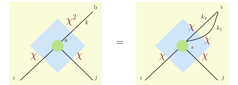
Figure 8. (color online) A leg k whose Hilbert space dimension is
$ \chi^2 $ can be reshaped into two legs$ k_1 $ and$ k_2 $ , whose Hilbert space dimensions are$ \chi $ . -
Here, we consider the potential applications of QMF/QMC to the MERA tensor network. One aspect must be carefully addressed. Generically, given a tensor network, we have the freedom to assign tensors in the network. MERA, however, is usually homogeneous. We typically place the same isometries and entanglers everywhere. If this is the case, instead of the first version of the QMF/QMC, we must adopt the second version. This leads to a problem: we cannot ensure whether there is a type of tensor that satisfies QMF = QMC. Fortunately, this equality holds asymptotically under specific conditions, as we discuss in Section 5.3.
Next, we suppose that all edges of the MERA are associated with the same Hilbert space dimension
$ \chi $ , and QMF = QMC is satisfied. We now consider an exclusive causal cone of region A as a sub network$ D_A $ of the entire network. The edges living on the UV cutoff of the network$ D_A $ are set to be inputs, while the edges emanating from the exclusive causal cone are regarded as outputs (details are shown in Fig. 7). For the MERA network, it is evident that the edges that are cut by the causal cone form a minimum cut set of the network$ D_A $ , because the number of edges living on a space-like cut is consistently larger than the one living on a causal cut. For simplification, we assume that the number of output edges is k so that the dimension of that Hilbert space(also QMC of this sub network) is equal to$ \chi^k $ . Then, we can simply obtain the quantum max-flow of$ D_A $ as$ \chi^k $ due to the QMF/QMC theorem.From Section 4.1, we know that the entanglement entropy between inputs and outputs for this network reaches its maximum
$ MEE(D_A) = \log\ {\rm QMC}(D_A) =$ $ \log\ \chi^k = k\log\ \chi $ . Clearly, this shows that the entanglement entropy is equivalent to counting the number of edges cut by the causal cut, where the weight of each edge is just$ \log\ \chi $ . That is to say, if a network satisfies the QMF/QMC theorem everywhere, then the flux of each edge would achieve its maximum value. Recalling our argument (38) and (44) in Section 2.1, Eq. (44) holds because of the QMF/QMC theorem, and one can obtain the flux of a causal diamond D by replacing QMF with QMC in Eq. (38)$\begin{split} {\cal D} =& - \left( {\int_{{D_{AB}}} \rho + \int_{{D_{BC}}} \rho - \int_{{D_{ABC}}} \rho - \int_{{D_B}} \rho } \right)\\ =& - \rho \left( {\int_{{D_{AB}}} + \int_{{D_{BC}}} - \int_{{D_{ABC}}} - \int_{{D_B}} {} } \right)\\ = & - \rho {V_D} = \log \frac{{{\rm QMC}({D_{AB}}) \cdot {\rm QMC}({D_{BC}})}}{{{\rm QMC}({D_{ABC}}) \cdot {\rm QMC}({D_B})}}. \end{split}$

(46) In the second line,
$ \rho $ is taken out from integral, because MERA has same isometries everywhere, so it is independent of$ (u,v) $ . The last line of Eq.(46) can be expressed as$ (k_{AB}+k_{BC}-k_{ABC}-k_B)\cdot \log\chi $ , where$ k_{AB} $ is the number of min-cut edges of$ D_{AB} $ , etc.Evidently, canceling incoming and outgoing flow will yield the flux
$ {\cal D} $ . In Ref. [9] the authors claimed that the number of remaining edges is equal to the number of isometries inside the diamond considered. This is the case where density$ \rho $ is a constant. Each isometry contains$ 1/(4G_N) $ bits of information. However,$ \rho(x) $ is related to location$ x $ in a tensor network when the type of isometries is unconstrained. A different isometry may contain a different number of bits, and the emerged space-time has an entirely different structure. If$ \rho $ is constant, Eq. (46) indicates that the number of isometries is directly proportional to the volume. This recovers the argument given in Ref. [9]. In that article, the density of compression of a compression network is proportional to the number density of isometries for a vacuum MERA. Based on these observations, the authors claimed that$ {\cal D}({\rm isometries}) = I(A,C|B) $ , which is a relation between the number of isometries and the corresponding volume. This statement is consistent with our argument given above (46), namely, as the QMF/QMC theorem holds for a given network,$ \rho V_D $ can be interpreted as the density of compression. From this point of view, physically,$ \rho $ can be viewed as density of isometries or equivalently density of compression.From Fig. 8(b) clearly shows that a causal diamond contains numbers of tilted chessboards, and each of them corresponds to an isometry. This implies that the volume of every minimum chessboard (or unit chessboard) is the same, because it contains only one isometry. This property is the key for the tensor network to have the geometry of
$ {\rm dS}_2 $ . This can be also obtained from Eq. (46), when D is an infinitesimal causal diamond. Indeed, it follows from Refs. [8, 9] and Eq. (46) that$\begin{split} {\rm d}{V_{\rm network}} = {\cal D} = |\rho |{V_D} = I(A,C|B) = 4\log \chi \cdot \dfrac{{{\rm d}u{\rm d}v}}{{{{(v - u)}^2}}}. \end{split}$

(47) We obtain the last equality in the following discussion. We can find directly that
$|\rho | = 2\log \chi .$

(48) -
In this subsection, we return to the discussion of the holographic entanglement entropy, in the framework of our flow language. Primarily, we should claim two important properties of this flow, which are useful in our following discussion. Considering a tensor network, which includes coarse-graining (or isometries), first we assume that the Hilbert space dimension of each edge is equal. For such a network, following the renormalization flow in each step of coarse-graining will reduce the number of edges. That means that in a causal domain D, the lower cut number is consistently larger than the upper cut number. We assume that the flow runs along the RG flow direction. The first property is that the flux of this region
$ \oint_{\partial D} f $ is always nonnegative, hence from Eq. (38),$\int_D \rho \leqslant 0.$

(49) The second property is apparently deduced from the first property. Suppose we have two regions A, B of the boundary, then the flux
$ {\cal D}_{AB} $ is consistently larger than the sum of$ {\cal D}_A $ and$ {\cal D}_B $ :$\int_{{D_{AB}}} \rho \leqslant \int_{{D_A}} \rho + \int_{{D_B}} \rho .$

(50) Generalization to more than two regions is the same. This inequality implies that
$ D_{AB} $ includes some densities of compression, which are not included in$ D_A $ and$ D_B $ . Indeed, these densities provide the conditional mutual information between A and B on the boundary, as shown in Ref. [9].For a given flow, it is simple to check from the second property that
$\begin{split} \int_{{C_{AB}}} f =& \int_{AB} f - \int_{{D_{AB}}} \rho \leqslant \int_A f - \int_{{D_A}} \rho + \int_B f - \int_{{D_B}} \rho \\ =& \int_{{C_A}} f + \int_{{C_B}} f . \end{split}$

(51) Returning to the MERA network, which properly exhibits these two properties, the RT formula is represented by
$S(A) = \max\int_{{C_A}} f ,$

(52) which is the maximum flux through the causal cut
$ C_A $ . We can simply denote it as$ \int_{C_A}f(A) $ . After using the second property (50), and choosing a flow$ f(AB) $ , which maximizes the flux through AB, we have$\begin{split} S(A) + S(B) \geqslant & \int_{{C_A}} f (AB) + \int_{{C_B}} f (AB)\\ \geqslant & \int_{{C_{AB}}} f (AB) = S(AB). \end{split}$

(53) This simply represents the subadditivity of the entanglement entropy. Similarly, for the case including three regions, we choose a flow
$ f(A,B,C) $ , which maximizes the flux through A, B, AB, BC, and ABC simultaneously. Eq. (49) leads to the strong subadditivity of the entanglement entropy$\begin{split} I(A:C|B) =& \int_{{C_{AB}}} f (A,B,C) + \int_{{C_{BC}}} f (A,B,C)\\ & - \int_{{C_B}} f (A,B,C) - \int_{{C_{ABC}}} f (A,B,C)\\ =& S(AB) + S(BC) - S(B) - S(ABC)\\ =& - \int_D \rho \geqslant 0. \end{split}$

(54) -
In this section, we attempt to provide further detail on the quantum bit threads model from a physical point of view. First, we show the meaning of
$ \rho(x) $ and some requirements of such local contribution of a certain conditional mutual information. Second, we find that because$ \rho = $ constant, the 2D space-time structure constructing by a coarse-graining tensor network is$ {\rm dS}_2 $ , which is the same as kinematic space. As mentioned above, to maintain the entanglement flow conserved, one has to introduce a density$ \rho $ of the isometry tensor. This can be observed when the QMF/QMC theorem holds. Generally,$ \rho $ depends on the position of isometry:$ \rho(x) $ and is related to the structure of tensor network (Fig. 9). From Eq. (45), the emerged manifold is determined by such density$ \rho(x) $ . For the MERA case,$ \rho $ is a constant, and the emerged space-time is scale invariant as discussed later (i.e., it is a de Sitter space-time). We can also obtain the relation of Hilbert dimension$ \chi $ and central charge c of boundary theory. Finally, we will talk about the role of the central charge c in QMF/QMC and space-time.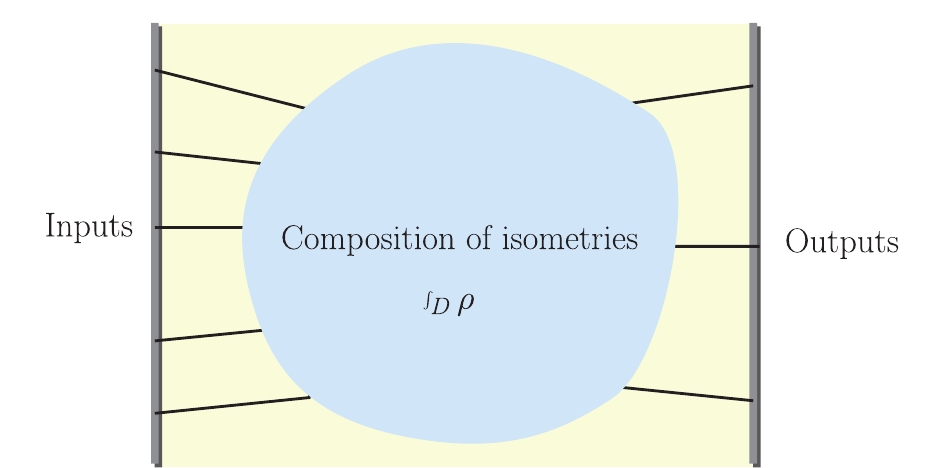
Figure 9. (color online) For a general tensor network, the emerged manifold is determined by the general density
$ \rho(x) $ -
In the previous section, we initially set up the quantum bit threads by defining
$ \rho $ in the tensor network. This can be understood as a source (or sink) that counts how many quantum bits are decompressed (or compressed) in the isometry. In this subsection, we attempt to provide more interpretation of such density in MERA.Recently, a concept called the “entanglement contour” of quantum systems has been studied in holography [15, 16]. In general, the contributions to entanglement entropy come from not only degrees of freedom near the boundary between A and
$ \bar{A} $ , but also degrees of freedom further away from this boundary. The entanglement contour$ s_A(x) $ is defined as a local quantity [15, 16]:$S(A) = \int_A {{s_A}} (x),$

(55) that aims to quantify how many degrees of freedom in region A contribute to the total entanglement entropy. In this paper, we propose that, similar to the entanglement contour, the density
$ \rho(x) $ contributes local degrees of freedom between two intervals to the total conditional mutual information. As mentioned in Section 3, the isometries encode the density of compression indicating the quantity of information (q-bits) sharing between two infinitesimal intervals$ [u-\Delta u, u] $ and$ [v, v+\Delta v] $ . Hence,$ \rho(x){\rm d}V $ encodes the conditional mutual information of a local degree of freedom only between local region$ [u-\Delta u, u] $ and$ [v, v+\Delta v] $ . We further find that such density$ \rho(x) $ satisfies some requirements similar to those of the entanglement contour [15, 16].The requirements of
$ \rho $ in the MERA tensor network is as follows. Here, we denote$ \rho_{D}(x) $ as the density of conditional mutual information$ I(A_1,A_3|A_2) $ , where D corresponds to the causal domain in the kinematic space of boundary subregion$ A_1\cup A_2\cup A_3\equiv A $ . Let us denote$ \tilde{\rho}_{D}(x) = -\rho_{D}(x) $ . Then the requirements of$ \tilde{\rho}_{D}(x) $ are given by:(1) Positivity:
$ \tilde{\rho}_{D}(x)\ge 0, \forall x\in D. $ (2) Normalization:
$ I(A_1,A_3|A_2) = \int_{D}\tilde{\rho}_{D}(x). $ (3) Invariance under symmetry transformations: Consider four sites
$ i_1,i_2 \in A_1 $ and$ j_1,j_2 \in A_3 $ and$ |j_1-i_1| = |j_2-i_2| $ . Let T be a symmetry of reduced density matrix$ \varrho_A $ , that exchanges two sites$ i,j\in A $ . After exchanging two points$ x_1,x_2\in D $ , where$ x_1 = (i_1,j_1), x_2 = (i_2,j_2) $ , we have$ \tilde{\rho}_D(x_1) = \tilde{\rho}_D(x_2) $ .(4) Invariance under local unitary transformations: If
$ \varrho'_A = U_X \varrho_A U_X^{\dagger} $ , where$ U_X $ is a local unitary transformation supported on$ X\subseteq A $ , then$ \tilde{\rho}_D (K) $ is equal for both$ \varrho_A $ and$ \varrho'_A $ .$ K\subseteq D $ is a causal domain corresponding to$ a_1\cup a_2\cup a_3 $ where$ a_1\subseteq A_1 $ and$ a_3\subseteq A_3 $ .(5) Upper bound: If we decompose D into a causal domain
$ D_{\Omega} $ and$ D_{\Omega}^- $ , and K is contained within$ D_{\Omega} $ , then${\tilde \rho _D}(K) \leqslant I({D_\Omega }),$

where
$ I(D_{\Omega}) $ is the conditional mutual information given by$ D_{\Omega} $ .In our toy model, requirements (1) and (2) have been discussed in the last section, see Eqs. (49) and (54). The positivity is due to the amount of isometry tensors in the MERA tensor network, and
$ \rho_D (x) $ is regarded as a sink in the network.Requirement (3) is actually the symmetry of the MERA tensor network. T is a symmetry of
$ \varrho_A $ , i.e.,$ T\varrho_A T^{\dagger} = \varrho_A $ , that exchange two sites. Therefore, if we exchange$ i_1\leftrightarrow i_2 $ and$ j_1\leftrightarrow j_2 $ at the same time, the system would remain unchanged. This requirement ensures that$ \tilde{\rho}_D(x) $ is the same on two points$ x_1 $ and$ x_2 $ of D.$ |j_1-i_1| = |j_2-i_2| $ implies$ x_1 $ and$ x_2 $ are two sites in the same layer of MERA tensor network. This reflects the translation symmetry of the quantum system, and$ \tilde{\rho}_D(x) $ plays an equivalent role in the MERA tensor network.Requirement (4) refers to the subregion K within region D. The definition of
$ \tilde{\rho}_D(K) $ is similar to the one of entanglement contour, which extends the density of single point to the density of a causal domain$ K\subseteq D $ :${\tilde \rho _D}(K) = \int_K {{{\tilde \rho }_D}} (x).$

(56) Similar to the entanglement contour [16], for two disjoint subsets
$ K_1,K_2\subseteq D $ , with$ K_1\cap K_2 = \emptyset $ , the density is additive:${\tilde \rho _D}({K_1} \cup {K_2}) = {\tilde \rho _D}({K_1}) + {\tilde \rho _D}({K_2}).$

(57) Then, if
$ K_1\subseteq K_2 $ , the density must be larger on$ K_1 $ than$ K_2 $ :${\tilde \rho _D}({K_1}) \leqslant {\tilde \rho _D}({K_2}),\;\;\;{\rm{if}}\;\;\;{K_1} \subseteq {K_2}.$

(58) This is the monotonicity of
$ \tilde{\rho}_D $ . These two properties are observed directly from the kinematic space.It can be learned from Eq. (43) that requirement (4) holds in our bit threads language. As we mentioned in Section 2.2 (below Eq. (16)), after choosing an appropriate basis, one can let
$ \beta $ under this basis be matrix C. Then, the reduced matrix$ \varrho_A = {\rm Tr}_{\bar{A}}|\alpha\rangle \langle\alpha| = CC^{\dagger}/{\rm Tr}(CC^{\dagger}) $ . The unitary transformation$ U_X $ is defined on a Hilbert space$ V_A\otimes V_{\bar{A}} $ , but only nontrivial on X. Hence, it does not affect$ \bar{X} = A-X\supseteq \bar{A} $ . After performing this unitary transformation, the reduced matrix is$ \varrho'_A = C'C'^{\dagger}/{\rm Tr}(C'C'^{\dagger})) $ .$ C' $ is the new matrix under the unitary transformation$ C' = U_X CU_X^{\dagger} =$ $ U_X CU_X^{-1} $ , i.e., matrix$ C' $ and C have the same rank. Therefore, the local unitary transformation does not affect the term$ \log \{{\rm rank}\; C\} $ in Eq. (43). Assuming that the causal domain K in the kinematic space is given by$ a_1\subseteq A_1 $ and$ a_3\subseteq A_3 $ on the boundary (Fig. 10). The subregion density on K is given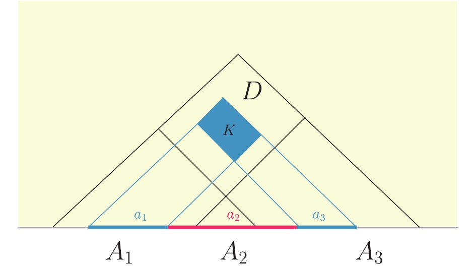
Figure 10. (color online) Sketch of causal domain in kinematic space.
${\tilde \rho _D}(K) = \int_{{D_{{a_1}{a_2}{a_3}}} + {D_{{a_2}}} - {D_{{a_1}{a_2}}} - {D_{{a_2}{a_3}}}} {{{\tilde \rho }_D}} (x) . $

(59) After applying formula (43), the second term
$ \int f $ in the left-hand side of Eq. (43) is cancelled, such that it cannot be affected by the unitary transformation. The remaining terms are the rank of matrix C, which are unchanged under the transformation. In summary, the density$ \tilde{\rho}_D (K) $ is invariant under unitary transformation. Requirement (5) is easy to obtain in our bit threads of the MERA tensor network. In this case,$ \tilde{\rho} $ is a constant, and we obtain${\tilde \rho _D}(K) = \int_K {{{\tilde \rho }_D}} (x) \leqslant \int_{{D_\Omega }} {{{\tilde \rho }_D}} (x) = \int_{{D_\Omega }} {{{\tilde \rho }_{{D_\Omega }}}} (x) = I({D_\Omega }).$

(60) -
The kinematic space of an
$ {\rm AdS}_3 $ time slice, which is equivalent to an auxiliary$ {\rm dS}_2 $ according to the first law of entanglement entropy [18, 19], can be constructed by the conditional mutual information of a boundary system.It follows from Eq. (46) that the conditional mutual information can be written as
$ \log_2\ \chi \cdot (k_{AB}\!+\!k_{BC}\!-\!k_{ABC}\!-\!k_{B}) $ , where$ k_{AB},\; k_{BC}\cdots $ are, respectively, the numbers of edges cut by$ C_{AB}, \;C_{BC} $ , etc. For such a coarse-graining tensor network, a region with length$ l_{AB} $ satisfies$ l_{AB}\cdot {\rm e}^{-k_{AB}/2} \sim 1 $ , namely,${k_{AB}} \simeq 2\log \;{l_{AB}}.$

(61) Consider the case where regions
$ A:(u-{\rm d}u,u) $ ,$ B:(u,v) $ , and$ C:(v,v+{\rm d}v) $ construct a volume element on$ (u,v) $ in the kinematic space. We obtain$\begin{split} {\rm d}{V_{\rm network}} \simeq & 2\log \chi \cdot \left[ {\log \frac{{(v - u + du)(v - u + {\rm d}v)}}{{(v - u + {\rm d}v + {\rm d}u)(v - u)}}} \right]\\ =& 2\log \chi \cdot \frac{{{\rm d}u{\rm d}v}}{{{{(v - u)}^2}}} + O({\rm d}u{\rm d}v), \end{split}$

(62) which is the conditional mutual information
$ I(A:C|B) = \partial_u\partial_v S_{\rm ent}(u,v){\rm d}u{\rm d}v $ . Comparing it with the entanglement entropy of the boundary interval$ (u,v) $ , i.e,$ S_{\rm ent} = (c/3)\log\ (v-u)/\epsilon $ , we have$\log \chi \simeq \frac{c}{6}.$

(63) One aspect requires further emphasis. The above discussion is applied in the planar coordinates of
$ {\rm dS}_2 $ . The topology is a plane$ \mathbb R^1 \times \mathbb R^1 $ rather than a cylinder$ \mathbb S^1 \times \mathbb R^1 $ . A plane implies that its cylinder circumference is significantly larger than the interval,$ \varSigma \gg (v-u) $ (actually it is infinite). Hence, if we consider a lattice model on the boundary, the number of sites in$ (v-u) $ is considerably lower than those in its complement$ (v-u)^c $ . If we do not distinguish the direction of geodesics in the$ {\rm AdS}_3 $ time slice, this kinematic space only covers a half of the full$ {\rm dS}_2 $ , which is the planar patch$ {\cal O}^+ $ (or$ {\cal O}^- $ ) [20, 21].However, we must note that the present flow model is a toy model in the sense that the edges are maximally entangled④, as mentioned in Section 4.1. Thus, the flow in each edge has the same flux and reach their maxima
$ \log\chi $ simultaneously. This is a strict constraint and only works for some special tensor networks, such as a prefect tensor [17] or random tensor [22]. A recent attempt in constructing a continuous tensor network based on path-integral optimizations [23, 24] may have clues to overcome this difficulty. For MERA, as an effective simulation for the ground state of real CFT, the entanglement entropy must not be maximal. However, one can control the degree of entanglement in MERA for approximating the real CFT [25]. We argue that under this control the corresponding space-time is still dS, but with different density$ \rho $ (Appendix A). -
The central charge c is a measure of the number of degrees of freedom. In a strong coupling limit of the field theory, when the number of degree of freedom is very large
$ c\sim N^2\gg 1 $ , the string interaction becomes weak, and we just consider the classical string limit [26, 27]. In such a limit we can discuss the dynamics of quantum CFT by studying a dual semiclassical gravitational physics in space-time.In Eq. (46), we take out
$ \rho $ from the integral, because we restricted all the isometries tensor in the tensor network of the same type. This corresponds to the second version of QMF/QMC conjecture, as we lose the freedom to assign tensors. In this circumstance, the QMF/QMC conjecture is not always valid, even when each edge has the same capacity, just like the MERA. Hence, we have a bound for QMF:$ {\rm QMF}(G,a) \leqslant {\rm QMC}(G,a) $ , i.e., the flux in each edge cannot reach its maximal capacity. This is what a MERA of a real CFT requires.Fortunately, recent work from Hastingss [28] demonstrated that this conjecture is “asymptotically” true in the limit as
$ \chi \rightarrow \infty $ . Hence, the ratio of the QMF to the QMC converges to one as$ \chi $ tends to infinity. We write$ {\rm QMF}(G, \chi, O) $ to denote the QMF for a given graph G with ordering O and capacity$ \chi $ in every edge. Ref. [28] showed that$ {\rm QMF}(G,\chi ,O) = {\rm QMC}(G,\chi ) \cdot \left( {1 - O(1)} \right).$

(64) In the higher-order term
$ O(1) $ , we consider as an asymptotic function of$ \chi $ , which may also depend on G and O. Eq. (63) this implies that the QMF/QMC conjecture is asymptotically true in a large central charge limit. The entanglement entropy$ S(A) = \int_{C_A} f $ is asymptotically equal to$ \log\ {\rm QMC} $ , and we can simply count the number of cut legs. We therefore have a dual classical, or at least semiclassical gravitational theory in the auxiliary$ {\rm d}S_2 $ space-time. This can be simplified in such a large c limit, and computations of entanglement entropy can be made by a holographic map to a volume in auxiliary space.We show that max-flow/min-cut in the classical network is always valid. This, however, fails for a tensor network: the quantum version of max-flow/min-cut conjecture does not hold in general, except for large
$ \chi $ . Hence, this result (64) indicates that a quantum phenomenon (QMF$ \neq $ QMC) disappears in the large system limit. This is our claim that the classical space-time can emerge from the tensor network model. The network becomes “classical”, and we can define the flow in it, which constructs the gravitational theory. This agrees with the argument that in the large c limit, the quantum fluctuations of emergent space-time can be effectively suppressed. This is evident from the relation$ c\sim\frac{1}{G_{N}} $ . We consider the large c limit, because we adopted the second version of QMF/QMC, whose tensor was restricted. This will result a nontrivial complexity of the MERA circuit. The duality between the tensor network and gravity in our model is supported from the point of view of complexity, which explains that the complexity corresponds to the gravitational action on the gravity side [29]. The quantum corrections may be considered in our toy model of the tensor network. These corrections correspond to corrections in the holographic entanglement entropy. We provide a brief discussion in the following section.Recently, the quantum Hamiltonian complexity has made rich connections to the physical system. Physicists are concerned about some properties of local Hamiltonian in the condensed system, such as the ground state or entanglement properties. In Ref. [8], it was shown that the quantum max-flow is related to the so-called quantum satisfiability problem,
$ {\rm QSAT} $ , which is defined as the quantum version of$ k-SAT $ in Ref. [30]. In some specific cases, the problem of QSAT and QMF were found to be equivalent. Thus, they yield a conjecture similar to one in QSAT, that the QMF/QMC conjecture holds when the Hilbert space dimensions of edges become very large. This conjecture was demonstrated in Ref. [28]. However, machine learning is also related to the tensor network through renormalization in condensed matter physics [31] and possibly has significant holographic meaning [32, 33]. Ref. [34] showed that the quantum max-flow provides a non-trivial measure of the ability of tensor network to model correlations in a so-called deep convolutional network. All of these imply a possible understanding on emergent gravity. -
By making use of the QMF/QMC theorem developed recently in the tensor network, we proposed a tensor network/flow correspondence, which is a quantum generalization of the flow description of the RT formula in Ref. [2]. Based on information-theoretic considerations, we suggest that for the MERA, we need to introduce a new variable
$ \rho $ , which is interpreted as the density of the tensor networks. Physically, this term is viewed as the source (or sink) of the tensor networks, and thus plays a significant role in the flow description of the RT formula.$ \rho(x = (u,v)) $ is a local contribution to a certain conditional mutual information between local degrees of freedom only in sites u and v. Its value is not only closely related to the geometric structure of the tensor network (equivalently, the metric of emergent space-times from the emergent point of view), but also the density of compression or decompression of quantum bits through reducing or expanding the dimension of Hilbert space, which implies a naive picture that the evolution of our universe can be regarded as a huge and complex quantum circuit. The density$ \rho $ is the main role for the space-time's construction in the large c limit. The MERA circuit is a program, which continuously entangles quantum bits, and the complexity$ {\cal C} $ is given by counting the number of entangled pairs in isometry in such a limit,${\cal C} \sim \int {\sqrt { - g} } \rho .$

(65) We can relate this complexity to the gravitational action of the de Sitter space, and
$ \rho $ plays the role of gravitational constant [29].Our proposal of quantum bit threads provides a new perspective on the holographic tensor network and is different from the one presented by Headrick-Freedman. The bit threads of Headrick-Freedman are constructed in an AdS time slice. However, we propose the quantum bit threads in kinematic space instead of its original AdS time slice. We would like to emphasize that the classical limit of our quantum version of bit threads is not the classical network of Headrick-Freedman's because of the difference between the quantum and classical networks (further details on the definition are provided in Ref. [8]).
We further consider the
$ 1/N $ quantum corrections to the quantum bit threads. The quantum corrections of holographic entanglement entropy have been studied in Ref. [35]. The QMF is asymptotically equal to QMC in the large c(or small$ 1/N^2 $ ) limit, as shown in Eq. (64). QMF is calculated by the input-to-output map$ \beta $ , or equivalently the matrix C. The entanglement entropy can be also obtained by matrix C, as shown in Eq. (18). Hence, the quantum corrections of quantum bit threads can be also studied in a similar way to the quantum corrections of HEE. We hope that further details of this quantum effect of bit threads can be studied in the future. -
If the tensor network is MERA, we know the entanglement entropy of the state with
$l $ sites has upper bound$\tag{A1}{S_{{\rm{MERA}}}}(l) \leqslant 4f(k){\log _k}l \cdot \log \chi ,$

(A1) where the interval is larger than the lattice spacing, i.e.,
$ l\gg1 $ .$ \chi $ is the the Hilbert dimension of each edge, k is the number of sites in a block to be coarse-grained, and$ f(k) $ is a function of k with$ f(k)\leqslant k-1 $ .$ \log\chi $ is the maximum entanglement entropy of a single edge when we trace out the rest of the MERA. It is instructive to introduce a parameter$ \eta\in[0,1] $ to describe the degree of entanglement [25]. Thus, the average entanglement entropy per edge in MERA is$ \eta\log\chi $ . Then, we can write the entanglement entropy as$\tag{A2}{S_{{\rm{MERA}}}}(l) = 4f(k){\log _k}l \cdot \eta \log \chi .$

(A2) Recalling that the entanglement entropy of CFT
$ S(l) = (c/3)\log l $ , then the MERA entropy (A2) yields a central charge$\tag{A3}c = \frac{{3L}}{{2{G_N}}} = 12\eta f(k)\frac{{\log \chi }}{{\log k}}.$

(A3) Because each edge has the same average entanglement entropy
$ \eta\log\chi $ we still can count the number cut by causal cut to obtain the entanglement of region$ l_0 $ . The auxiliary space-time given by MERA is still a de Sitter, but with the relation between$ \chi $ and central charge c Eq. (A3) different from Eq. (63). -
We should point out is that in Ref. [36], the authors define the entanglement density in
$ (1+1) $ -dimensional CFT. The entanglement density$ n(l, \xi, t) $ is defined by counting the number of entanglement pairs between the two points$ x = \xi-l/2 $ and$ x = \xi+l/2 $ . After comparison with the result of entanglement entropy in CFT2 they find$\tag{B1}{n_{\rm CFT}}(l,\xi ,t) = \frac{c}{{6{l^2}}},$

(B1) where c is the central charge, and l is the range of subsystem we consider. The horizontal ladders are the disentanglers, which are unitary transformations between two spins. Each disentangler carries the entanglement entropy
$ \log 2 $ between these two spins. The number of disentanglers in each bond$ N(l,\xi,t) $ is roughly given by [36]$\tag{B2}N(l,\xi ,t) \simeq {n_{\rm CFT}}(l,\xi ,t) \cdot {l^2} = \frac{c}{6},$

(B2) which can be understood as the density of disnentanglers.
Although this expression of density of disentanglers looks highly similar to our density of compression,
$ \rho\propto N(l,\xi,t) = c/6 $ . We claim that they have a different meaning. First, in Ref. [36], the MERA is defined in a time slice of AdS space. However, in favor of Ref. [9], which is the premise of our paper, the MERA lives on the kinematic space rather than the time slice of the AdS. The kinematic space is a dS2, which has a natural causal relation between tensors. Second,$ N(l,\xi,t) $ is the density of disentanglers in each bond, whereas$ \rho $ is the density of compression in each isometry. Third,$ N(l,\xi,t) $ is the number of disentanglers in each bond, which describes how many entanglement pairs are in such a bond. Thus, to obtain the entanglement entropy of a subsystem, one can roughly count the number of intersecting bonds and multiply the density$ N(l,\xi,t) $ . In contrast, in our study we define the density$ \rho $ from an information point of view. The volume of kinematic space is the conditional mutual information, which shares the information between two regions. The$ \rho $ describes the quantity of information that will be shared, or be compressed along the quantum circuit, which have a different meaning regarding the density of disentanglers. To obtain the conditional mutual information, we can count the isometry number and multiply the density$ \rho $ .We would like to thank Tadashi Takayanagi for reading and commenting on the paper. We are also grateful to Wen-Cong Gan and Bo Xiong for useful discussions.
Quantum bit threads of MERA tensor network in large c limit
- Received Date: 2020-02-11
- Available Online: 2020-07-01
Abstract: The Ryu-Takayanagi (RT) formula plays a large role in the current theory of gauge-gravity duality and emergent geometry phenomena. The recent reinterpretation of this formula in terms of a set of “bit threads” is an interesting effort in understanding holography. In this study, we investigate a quantum generalization of the “bit threads” based on a tensor network, with particular focus on the multi-scale entanglement renormalization ansatz (MERA). We demonstrate that, in the large c limit, isometries of the MERA can be regarded as “sources” (or “sinks”) of the information flow, which extensively modifies the original picture of bit threads by introducing a new variable ρ: density of the isometries. In this modified picture of information flow, the isometries can be viewed as generators of the flow. The strong subadditivity and related properties of the entanglement entropy are also obtained in this new picture. The large c limit implies that classical gravity can emerge from the information flow.


 DownLoad: