


 Abstract
 HTML
HTML Reference
 Related
 PDF
PDF


-
Conformal field theories constitute an important subset of quantum field theories owing to their extended symmetry algebra, which includes in particular the scale transformation. Because of scale invariance, conformal field theories are crucial in the study of critical phenomena near the phase transition. Another reason why there has been significant interest on conformal field theory over the past few decades is the holographic principle, in particular the AdS/CFT correspondence [1]. According to it, a strongly-coupled conformal field theory with a large number of degrees of freedom can have a dual description as a weakly-coupled Einstein-like gravity in one higher spacetime dimensions. For careful discussions on the requirement for the conformal field theory to have a gravity dual, see e.g. [2, 3]. Operators in conformal field theory have their dual fields in the gravity counterpart, and an elaborate prescription for calculation of correlation functions thereof has been established and passed a number of non-trivial tests [4].
Subsequently, researchers attempted to turn on some deformation in the duality pairs to break the scale invariance and see if the correspondence still holds. Janus configuration [5,6] is one of the most interesting examples, where we select a relevant operator and make the dual field in AdS side position-dependent. Typically we introduce a co-dimension one defect, or interface, and different values for scalars on each side implies that some of the coupling constants jump across the interface. For the first example considered in [5], on the gauge theory side, we have
$ {\cal N} = 4 $ super Yang-Mills theory in 3+1 dimensions, and across the 2+1 dimensional interface the gauge coupling assumes different values. On the gravity side, we have to consider so-called domain wall-like solutions, and due to the inherent nonlinearity of Einstein gravity, the field equations are typically reduced to a system of non-linear ordinary differential equations. To obtain an exact solution is thus usually not possible because of nonlinearity. Indeed, most previous studies on the construction of Janus solutions on the gravity side have relied on numerical integration [6-21]. Notable exceptions include the$SO(4)\times SO(4)$ -symmetric truncated model in Sec. 3.1 and theintegrable BPS equations in a recent work [22].Recently, we proposed a new perturbative approach for similar systems of non-linear ordinary differential equations derived from Einstein gravity coupled to scalar fields, in the context of AdS/CFT correspondence [23]. This technique was successfully applied to several Einstein-scalar systems in Euclidean signature space [23-25] which describes mass deformations of several dual conformal field theories in the large-N limit [26-30]. In particular, the matching of the sphere partition function for
$ {\cal N} = 2^* $ mass-deformed super Yang-Mills and its supergravity dual is now more firmly established through exact evaluation of a few leading-order expansion coefficients [23]. For$ {\cal N} = 1^* $ deformations, the first non-trivial coefficients in the series of expansion of the sphere partition function is analytically computed [24]. For the duality proposal of mass-deformed Brandhuber-Oz theory [31], we managed to re-sum the series expansion form of the sphere partition function as a function of mass and argued that the result does not agree with the large-N limit of the field theory side computation [23]. The main goal of this study is to illustrate that the same technique can also be successfully applied to holographic Janus solutions. Using our semi-analytic solutions, we calculate the holographic entanglement entropy [32,33] as a function of the perturbation parameter, which controls the magnitude of the deformation away from the AdS vacuum.Let us explain the setup in more detail. We will consider, for concreteness, the Janus solutions in three consistently truncated Einstein-scalar systems from
$ {\cal N} = 8,\, D = 4 $ maximal supergravity with the$ SO(8) $ gauge group [34]. The dual field theory is the well-known Chern-Simons matter theory living on M2-branes, the action of which was first explicitly written down by Aharony, Bergman, Jafferis, and Maldacena (ABJM) in Ref. [35]. Instead of the full$ SO(8) $ gauged supergravity, we are interested in various truncated models, focusing on specific mass deformations. Such truncated supergravity models were constructed and analyzed in Ref. [7], which we closely follow and consider the BPS equations presented thereof. We are only concerned with the bosonic sector, as we seek classical solutions. All three models have a single complex scalar field, which is invariant under a certain subgroup of the global symmetry$ SO(8)\subset E_{7(7)} $ . They will be referred to as$ SO(4)\times SO(4) $ ,$ SU(3)\times U(1)\times U(1) $ , and$ G_2 $ models. The scalar fields, although they are consistently referred to as z to maintain the generality of the discussion, are dual to different mass terms in the ABJM theory, which preserves the different symmetry subgroup of$ SO(8) $ that is the R-symmetry of the dual supersymmetric field theory. We are interested in conformal defects, which means that the Lorentz symmetry along the defect is also promoted to conformal symmetry, and our gravity ansatz is$ {AdS}_3 $ -sliced, instead of the Minkowski space. We treat the scalar fields as perturbation and solve the field equations exactly at each order. The boundary condition we impose is that the solution must be asymptotically$ {AdS}_4 $ in UV, and regular in IR.The utility of the perturbative approach is best illustrated when holographic calculations are compared to the field theory side result using supersymmetric localization [36], where we take the Euclidean signature and place the theory typically on the sphere. This was the reason the BPS equations in [26–30] were obtained in the Euclidean signature with the sphere-sliced metric ansatz. In contrast, Janus solutions in holography are constructed in Lorentzian signature, so it is not clear to us whether we can compare the result to a localization computation result. We thus choose to calculate holographic entanglement entropy, which is the minimal area of a spatial surface [32,33]. Although we do not attempt to do the field theory side computation in this article, we believe it should be possible, at least in weakly-coupled regime and simple geometry of the entanglement region, using e.g. the replica trick [37] and explicit form of the ABJM action.
This paper is constructed as follows. In Sec. 2, we introduce the notation and present the Einstein-scalar actions and their associated BPS equations. Section 3 is the main part, where we solve the BPS equations treating scalar fields as perturbations to AdS vacuum. We also consider the backreaction, and higher order solutions with the right boundary condition are also obtained analytically. In Sec. 4, we calculate the holographic entanglement entropy for Janus solutions constructed in Sec. 3, again solving the minimal-surface condition perturbatively. We conclude in Sec. 4 with discussions.
-
In this section, we closely follow and summarize the setup in Ref. [7], as a preparation for our perturbative analysis that will be presented in the following section. The authors of Ref. [7] presented three distinct subsectors of
$ {\cal N} = 8 $ ,$ SO(8) $ -gauged supergravity in$ D = 4 $ , by requiring invariance under certain symmetry subgroups of the global symmetry$ E_{7(7)} $ . They all have a complex scalar field coupled to Einstein gravity, and schematically share the following form.$ e^{-1}{\cal L} = \frac{1}{2} R - {\cal K}_{z \bar z} z' {\bar z}' - g^2 {\cal P}(z,\bar z). $

(1) In the above, e denotes the Jacobian determinant of the metric tensor, g is the gauging parameter, i.e., coupling constant, and
$ {\cal P} $ is the scalar potential. The actions enjoy the$ {\cal N} = 1 $ supergravity structure in four dimensions when the fermionic sector is appropriately added, and the complex scalar z with conjugate$ \bar z $ parameterize a Kähler manifold$ SL(2,\mathbb{R})/SO(2) $ , with a Kähler potential$ {\cal K} = - k \log (1-z\bar z). $

(2) The metric in the internal space is conventionally calculated by
$ {\cal K}_{z\bar z} = \partial_z \partial_{\bar z} {\cal K} = k/(1-z \bar z)^2 $ , and k is a constant that indicates the representation in which$ SL(2,\mathbb{R}) $ is embedded inside the larger symmetry group$ E_{7(7)} $ of$ {\cal N} = 8 $ gauged supergravity in four-dimensions. In contrast, the scalar potential is given in terms of the holomorphic superpotential$ {\cal V}(z) $ ,$ {\cal P} = e^{\cal K}({\cal K}^{z \bar z} \nabla_z {\cal V} \nabla_{\bar z} \bar {\cal V} -3 {\cal V} \bar {\cal V}) = 4 {\cal K}^{z \bar z}\partial_z W\partial_{\bar z} W -3 W^2 , $

(3) where
$ W\equiv \sqrt{e^{\cal K} {\cal V} \bar {\cal V}} $ . In Ref. [7], the authors considered the dual of a specific linear combination of mass terms on the gauge field theory side, preserving$ SO(4)\times SO(4) $ ,$ SU(3)\times U(1)\times U(1) $ , and$ G_2 $ symmetry, respectively. Although we use the same symbol, one should keep in mind that$ z,\bar{z} $ are thus dual to different mass terms in the dual field theory. For each model, the essential information is given in the table below.$ { SO(4)\times SO(4)} $ 

$ { SU(3)\times U(1) \times U(1)} $ 

$ {G_2} $ 

k 1 3 7 $ {\cal V}/\sqrt{2} $ 

$ 1 $ 

$ z^3+1 $ 

$ z^7 +7 z^4+7 z^3+1 $ 

We turn to the metric ansatz and the associated BPS equations. Physically, we are interested in co-dimension one conformal interfaces, so the spacetime is required to include
$ AdS_3 $ . We choose the following metric ansatz:$ {\rm d}s^2_4 = {\rm d}\mu^2 +{e}^{2A(\mu)} \, {\rm d}s^2(AdS_{3}) , $

(4) where
$ {\rm d}s^2(AdS_3) = {\rm d}r^2-\cosh^2(r/ \ell){\rm d}t^2+\sinh^2(r/ \ell) \ell^2 {\rm d}\phi^2 $ , with curvature radius$ \ell $ . When$ e^{2A} = (L/\ell)^2\cosh^2(\mu/L) $ , the above metric becomes exactly$ AdS_4 $ with curvature radius L.Using the standard parametrization
$ z: = e^{i\zeta}\tanh\alpha $ , one can easily verify that the field equations of (1) are reduced to the following one-dimensional action:$ {\cal L} = e^{3A} \left[3 (A')^2 -k\left[(\alpha')^2+\frac{1}{4} \sinh^2(2 \alpha) (\zeta')^2\right]-g^2 {\cal P} \right]-\frac{3}{\ell^2}e^{A}, $

(5) where
$ (\bullet)' = {{\rm d}(\bullet)}/{{\rm d}\mu} $ . The scalar potential can be written in terms of superpotential W$ \begin{aligned} {\cal P} = \frac{1}{k} \left[\left(\frac{\partial W}{\partial \alpha}\right)^2 +\frac{4}{\sinh^2 (2 \alpha)}\left(\frac{\partial W}{\partial \zeta}\right)^2 \right]-3 W^2 . \end{aligned} $

(6) One can also substitute the ansatz into the Killing spinor equations and demand the existence of non-trivial solutions. The analysis of Ref. [7] concludes that the following first-order differential relations,
$ \alpha' = -\frac{1}{2k} \left(\frac{A'}{W^2}\right)\frac{\partial W^2}{\partial \alpha}+ \frac{\kappa}{k}\left(\frac{e^{-A}}{\ell}\right) \frac{1}{\sinh (2 \alpha)}\frac{1}{W^2} \frac{\partial W ^2} {\partial \zeta}, $

(7) $ \zeta' = -\frac{2}{k} \left(\frac{A'}{W^2}\right)\frac{1}{\sinh^2 (2\alpha)}\frac{\partial W^2}{\partial \zeta}- \frac{\kappa}{k}\left(\frac{e^{-A}}{\ell}\right) \frac{1}{\sinh (2 \alpha)}\frac{1}{W^2} \frac{\partial W^2 } {\partial \alpha}, $

(8) are sufficient for supersymmetry and the field equations to be satisfied when combined with a constraint
$ \begin{array}{l} (A')^2 = g^2 W^2-\ell^{-2}e^{-2A} . \end{array} $

(9) For all truncated models, we consider that at trivial
$ {AdS}_4 $ vacuum the scalar fields$ \alpha,\zeta $ vanish, and their field equations are trivially satisfied. In contrast, Eq. (9) is satisfied for$ e^{2A} = (L/\ell)^2\cosh^2(\mu/L) $ , where L is related to the vacuum value of$ W = \sqrt{2} $ and$ L^{-1} = \sqrt{2}g $ .$ \kappa = \pm 1 $ is associated with the choice of the Killing spinor projection rule, and we take$ \kappa = -1 $ for concreteness. This solution, when uplifted corresponds to$ {{ {AdS}}}_4\times S^7 $ in$ D = 11 $ supergravity with maximal supersymmetry. There are additional AdS4 vacua in$ G_2 $ symmetric case, which will be considered in Sec. 3.3.Our strategy is, as illustrated in Refs. [23-25], to handle the BPS equations perturbatively. The AdS vacuum is treated as a reference solution at zeroth order, and scalar excitations will be treated as small perturbations at first, and their backreaction to the metric as well as their self-interaction will be studied iteratively order-by-order in the perturbation parameter. There is a subtlety though. It seems that the phase part of the scalar,
$ \zeta $ , is given a non-trivial kink-like profile already at zeroth order. Because the modulus$ \alpha $ will be kept zero at zeroth order, this does not make the entire complex scalar z non-vanishing, but this type of zeroth order deformation is essential for non-trivial Janus-like solutions.Furthermore, there will be in general three integration constants we can turn on for the single-scalar models of our interest. Among them, what is most crucial is the one corresponding to the strength of the perturbation, while the remaining two are location of the center of Janus in the spacetime and the internal
$ (\alpha,\zeta) $ -space. This property is to be contrasted with the supergravity solutions for the mass-deformed partition function [23-25], where each integration constant is dual to a mass parameter on the field theory side. -
In this case,
$ k = 1 $ and it seems that one can integrate the BPS equations exactly. Thus, this example serves as a touchstone for the utility of our proposed method, just like the perturbative re-construction of exact solutions [26] in the holographic mass-deformed ABJM theory [23]. The scalar potential and the superpotential are$ {\cal P} = -2 (\cosh 2 \alpha +2), \quad {\cal W} = \sqrt{\frac{2}{1-|z|^2}} . $

(10) The action allows a conserved Noether charge, because it is independent of
$ \zeta $ .$ Q = e^{3A}\sinh^2(2 \alpha) \zeta' = {\rm const}. $

(11) We will be able to express this integration constant in terms of the perturbative parameter. According to the analysis of Ref. [7], the BPS equations are, in addition to the universal constraint (9),
$ \alpha ' = -\tanh \alpha A', $

(12) $ \zeta ' = \frac{e^{-A} }{\ell}{\rm{sech}}^2\alpha. $

(13) They are easily integrated [7], and the branch of solutions that include the AdS vacuum take the following form.
$\begin{split} e^{A(\mu)} =& \frac{\sqrt{1-a^2}}{\sqrt{2} g \ell} \cosh(\sqrt{2}g(\mu-\mu_{\rm IR})), \\ \sinh \alpha =& \frac{a}{\sqrt{1-a^2}}\frac{1}{\cosh(\sqrt{2} g(\mu-\mu_{\rm IR}))}, \label{esol} \\ \tan (\zeta-\zeta_{\rm IR}) =& \sqrt{1-a^2}\sinh (\sqrt{2} g (\mu-\mu_{\rm IR})).\end{split} $

(14) Here, we have three integration constants, as already mentioned:
$ a<1 $ represents the strength of the deformation, and together with$ \zeta_{\rm IR} $ they determine the size and direction of the Janus configuration in the internal space$ (\alpha,\zeta) $ .$ \mu_{\rm IR} $ denotes the center of the Janus along the$ \mu $ -direction.Let us illustrate how these solutions can be constructed perturbatively. Using the form of AdS vacuum and also from the consideration of scalar fluctuation equations, we find that the following expansion in
$ \epsilon $ is most convenient.$ \begin{split} \alpha(\mu) =& {\rm{sech}} \left(\frac{\mu}{L}\right) \sum\limits_{ {\rm odd} \, n\ge 1} \alpha_n(\mu)\epsilon^n, \quad \zeta(\mu) = \sum\limits_{ {\rm even} \, n\ge 0} \zeta_n (\mu)\epsilon^n , \label{ansatz1} \\ e^{A(\mu)} =& \frac{L}{\ell}\cosh\left(\frac{\mu}{L}\right)\left(1+\sum\limits_{ {\rm even} \, n\ge 2} {\cal A}_n(\mu)\epsilon^n\right). \end{split} $

(15) The restriction to odd/even powers is possible owing to the invariance under
$ \alpha\rightarrow -\alpha $ , and when one utilizes the re-parametrization freedom of$ \epsilon $ . This implies that$ e^A,\alpha $ are even functions in$ \mu $ . In the above ansatz, we are restricted to the case where the position of the Janus defect$ \mu_{\rm IR} $ is small: we will see shortly that$ \mu_{\rm IR}\sim {\cal O}(\epsilon^2) $ can be included. We substitute Eq. (15) into the BPS equations and demand they are satisfied for all$ \epsilon $ .Equating zeroth order terms in
$ \epsilon $ , we have$ \zeta_0(\mu) = \zeta_*+\tan ^{-1}\left(\sinh \left(\frac{\mu}{L}\right)\right), $

(16) where
$ \zeta_* $ is an arbitrary real number that yields the value of$ \zeta $ at IR. At first order in$ \epsilon $ , the equation for$ \alpha_1 $ is, up to rescaling of$ \epsilon $ ,$ \alpha_1(\mu) = 1 . $

(174) Then at second order in
$ \epsilon $ , we have$ \zeta_2(\mu) = \zeta_{(2)}-\mu_{(2)}{\rm{sech}}\left(\frac{\mu}{L}\right) -\frac{1}{2} \tanh \left(\frac{\mu}{L}\right) {\rm{sech}}\left(\frac{\mu}{L}\right), $

(18) $ {\cal A}_2(\mu) = -\frac{1}{2} - \mu_{(2)} \tanh\left(\frac{\mu}{L}\right), $

(19) where
$ \zeta_{(2)} $ ,$ \mu_{(2)} $ are integral constants. The constant$ \mu_{(2)} $ is related to the integration constant in (14) via$ \mu_{\rm IR} = \mu_{(2)} \epsilon^2 $ . In contrast,$ \zeta_{(2)} $ can be absorbed into$ \zeta_* $ . The third order solution for$ \alpha $ is$ \alpha_3(\mu) = \alpha_{(3)}+\frac{\mu_{(2)}}{2} - \frac{1}{6} {\rm{sech}}^2\left(\frac{\mu}{L}\right). $

(20) Because
$ \alpha_{(3)} $ is the homogeneous solution, we can freely choose its value and set it to zero. This amounts to identifying$ a = \epsilon $ , and we can obviously continue to do this to higher orders and rediscover (14). In particular, one can check that$ e^{A} $ is just a constant$ (\sqrt{1-\epsilon^2}) $ times the zeroth order solution (except for a shift by$ \mu_{\rm IR} $ ). We also verify that the Noether charge is indeed constant, and consistent with$ \zeta'e^{3A}\sinh^22\alpha = 2a^2 g^{-2}\ell^{-3}, $

(21) up to
$ {\cal O}(\epsilon^{10}) $ . -
In this case, the scalar potential and the real superpotential are given as follows,
$ {\cal P} = -6 \cosh 2 \alpha, \quad {\cal W} = \frac{\sqrt{2} (z^3+1) }{(1-|z|^2)^{3/2}} , $

(22) with
$ k = 3 $ . As$ {\cal P} $ is independent of$ \zeta $ here, we have a Noether charge.$ Q = \zeta'e^{3A}\sinh^2 2\alpha . $

(23) The BPS equations are, in addition to the universal constraint (9),
$\begin{split} \alpha '=& -\frac{\sinh \alpha \cosh \alpha (\sinh 4\alpha \cos 3\zeta+\cosh 4\alpha+3)}{2 W^2}A'\\&+\frac{ e^{-A} \sinh ^22\alpha \sin 3\zeta}{2 \ell W^2}, \end{split}$

(24) $ \zeta ' = \frac{ \sinh 2\alpha \sin 3\zeta}{W^2}A'+\frac{ e^{-A} (\sinh 4\alpha \cos 3\zeta+\cosh 4\alpha+3)}{ 2 \ell W^2 }. $

(25) We note that the real superpotential W is given as
$ W^2 = \left(4 \sinh ^32\alpha \cos 3\zeta+15 \cosh 2\alpha+\cosh 6\alpha\right)/8. $

(26) Unlike the
$ SO(4)\times SO(4) $ -symmetric case, these equations are difficult to solve exactly. Since$ W^2 $ is not even under$ \alpha\rightarrow -\alpha $ , it is not an even function in$ \mu $ , and our perturbation ansatz is given as follows (i.e. perturbative modes of$ \alpha $ are not restricted to odd powers of$ \epsilon $ any more, and the modes of$ \zeta $ include even as well as odd powers).$\begin{split} \alpha(\mu) =& {\rm{sech}}\left(\frac{\mu}{L}\right)\sum\limits_{n = 1} \alpha_n(\mu)\epsilon^n, \\ \zeta(\mu) =& \sum\limits_{n = 0} \zeta_n (\mu)\epsilon^n , \\ e^{A(\mu)} =& \frac{L}{\ell}\cosh\left(\frac{\mu}{L}\right)\left(1+\sum\limits_{n = 1} {\cal A}_n(\mu)\epsilon^n\right). \end{split}$

(27) Note that
$ W^2 $ is$ {\cal O}(\epsilon^2) $ , which implies the$ {\cal O}(\epsilon^0) $ part of the equation is exactly the same as the$ SO(4) \times SO(4) $ model and we have again$ \zeta_0 (\mu) = \zeta_*+ \tan ^{-1}\left(\sinh \left(\frac{\mu}{L}\right)\right) . $

(28) Naturally, the equations for
$ \alpha, A $ are satisfied at$ {\cal O}(\epsilon^0) $ for vacuum configurations.We find the following solutions for
$ {\cal O}(\epsilon) $ .$ \alpha_1 (\mu) = \alpha_{(1)},\quad\quad\quad\quad\quad\quad\quad\quad\quad\quad\quad\quad\;\, $

(29) $\begin{split} \zeta_1(\mu) =& \zeta_{(1)}+\alpha_{(1)}{\rm{sech}}^2\left(\frac{\mu}{L}\right) \left(\sinh \left(\frac{\mu}{L}\right) \cos 3 \zeta_*\right.\\&\left.-\sinh^2\left(\frac{\mu}{L}\right)\sin 3 \zeta_*\right), \end{split}$

(30) $ {\cal A}_1(\mu) = -\mu_{(1)}\tanh \left(\frac{\mu}{L}\right).\quad\quad\quad\quad\quad\quad\quad\quad\;\, $

(31) Without losing generality, we can set
$ \alpha_{(1)} = 1 $ , and$ \zeta_{(1)} $ can be set to zero, as it can be absorbed into re-definition of$ \zeta_* $ . And$ \mu_{(1)} $ can likewise be set to zero, as it corresponds to the translational freedom in$ \mu $ .Substituting the
$ {\cal O}(\epsilon) $ results into$ {\cal O}(\epsilon^2) $ equations and proceeding in the same manner, we have$ \alpha_2(\mu) = {\rm{sech}}^2\left(\frac{\mu}{L}\right) \left(\sinh \left(\frac{\mu}{L}\right) \sin 3 \zeta_*- \cos 3 \zeta_*\right), $

(32) $\begin{split} \zeta_2(\mu) =& \tanh ^4\left(\frac{\mu}{L}\right) \sin 6 \zeta_*\\&+\frac{1}{4} \left(1-3 \cosh \left(\frac{2\mu}{L}\right)\right) \tanh \left(\frac{\mu}{L}\right) {\rm{sech}}^3\left(\frac{\mu}{L}\right) \cos 6 \zeta_*, \end{split}$

(33) $ {\cal A}_2(\mu) = -\frac{3}{2} . $

(34) We again made use of the re-definition freedom of
$ \epsilon $ , and the integral constant for$ {\cal A}_2 $ is fixed as we require$ A' = 0 $ at$ \mu = 0 $ .At the third order in
$ \epsilon $ , we find$ \begin{split} \alpha_3(\mu) =& \frac{1}{48} {\rm{sech}}^4\left(\frac{\mu}{L}\right) \left[6 \left(\sinh \left(\frac{\mu}{L}\right)-3 \sinh \left(\frac{3\mu}{L}\right)\right) \sin 6 \zeta_*\right. \\ &\left.+6 \left(7 \cosh \left(\frac{2\mu}{L}\right)+3\right) \cos 6 \zeta_*-20 \cosh ^2\left(\frac{\mu}{L}\right)\right], \end{split} $

(35) $ \begin{split} \zeta_3 (\mu) =& \frac{1}{24} \left({\rm{sech}}\left(\frac{\mu}{L}\right) \left(16 {\rm{sech}}^3\left(\frac{\mu}{L}\right)-45 {\rm{sech}}\left(\frac{\mu}{L}\right)\right.\right.\\&+32\bigg)-3\bigg)\sin 3 \zeta_* +\frac{1}{24} \left(32 {\rm{sech}}^6\left(\frac{\mu}{L}\right)-96 {\rm{sech}}^4\left(\frac{\mu}{L}\right)\right.\\&\left.+99 {\rm{sech}}^2\left(\frac{\mu}{L}\right)-35\right)\sin9 \zeta_* +\frac{1}{24} \tanh \left(\frac{\mu}{L}\right) {\rm{sech}}\left(\frac{\mu}{L}\right) \\&\times\left(16 {\rm{sech}}^2\left(\frac{\mu}{L}\right)-31\right)\cos3\zeta_* +\frac{1}{24} \tanh \left(\frac{\mu}{L}\right) {\rm{sech}}\left(\frac{\mu}{L}\right)\\&\times \left(32 {\rm{sech}}^4\left(\frac{\mu}{L}\right)-80 {\rm{sech}}^2\left(\frac{\mu}{L}\right)+63\right)\cos9 \zeta_*, \end{split} $

(36) $ \begin{split} {\cal A}_3(\mu) =& -\frac{4}{3} \tanh\left(\frac{\mu}{L}\right) \left({\rm{sech}}^3\left(\frac{\mu}{L}\right)-1\right)\sin3 \zeta_* \\ &+\frac{1}{6} \left(2 \cosh \left(\frac{2 \mu}{L}\right)+\cosh \left(\frac{4 \mu}{L}\right)+9 \right) {\rm{sech}}^4\left(\frac{\mu}{L}\right)\cos3\zeta_* . \end{split} $

(37) We do not present the solutions at higher orders, however it is evident that it is just the repetition of a similar integration problem. Using the higher-order results, the Noether charge is found to be
$ \begin{split} \zeta'e^{3A}\sinh^2 2\alpha =& \frac{4 L^2 }{\ell^3}\epsilon ^2-\frac{4 L^2 }{\ell^3}\cos (3 \zeta_*)\epsilon ^3\\&+\frac{6 L^2}{\ell^3} (\cos (6 \zeta_*)-3)\epsilon ^4 \\&+\frac{L^3 }{6 \ell^3} (64 \sin (3 \zeta_*)\\&+235 \cos (3 \zeta_*)-63 \cos (9 \zeta_*))\epsilon ^5\\& +{\cal O}\left(\epsilon ^6\right). \end{split} $

(38) Note that this is dependent on
$ \zeta_* $ , the initial condition of$ \zeta $ . The phase still changes by$ \pi $ between$ \mu = -\infty $ and$ \mu = \infty $ , as in the previous case of$ SO(4)\times SO(4) $ .$ \Delta\zeta: = \lim_{\mu \rightarrow \infty} ( \zeta(\mu)-\zeta(-\mu) ) = \pi+ {\cal O}(\epsilon^7). $

(39) One can draw various Janus curves in the
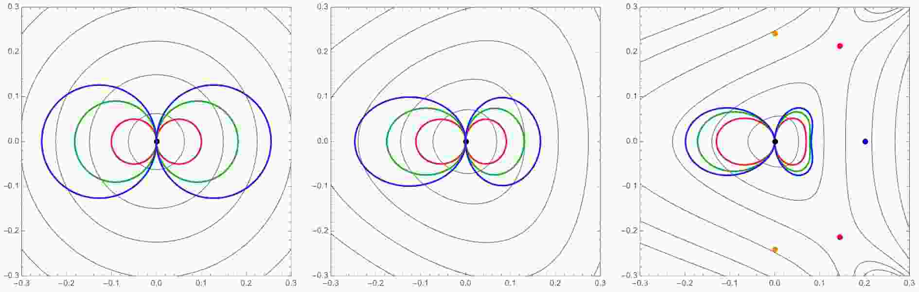
$ (\alpha\cos\zeta,\alpha\sin\zeta) $ -plane, and some samples are presented in Fig. 1. Because all the solutions flow to$ \alpha = 0 $ as$ \mu\rightarrow\pm\infty $ , they make a contractible loop. When compared with the plots presented in Ref. [1], our perturbative method restricts us to solutions homotopic to the AdS vacuum, whereas otherwise we find good agreements. Having$ \Delta\zeta = \pi $ for$ SO(4)\times SO(4) $ and$ SU(3)\times U(1)\times U(1) $ implies that the points at$ \mu = \pm\infty $ are smoothly joined at$ z = 0 $ . As we will see in the following subsection, this is not the case for$ G_2 $ .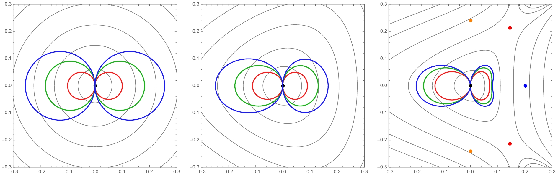
Figure 1. (color online) From left to right, the figures illustrate Janus solutions in polar coordinates of
$ \alpha e^{i\zeta} $ , for$ SO(4)\times SO(4) $ ,$ SU(1) \times U(1) \times U(1) $ , and$ G_2 $ -symmetrically truncated models, respectively. Different colors denote different values of$ \epsilon $ , i.e.$ 0.1, 0.18, 0.25 $ for$ {SO(4)\times SO(4)} $ ,$ 0.1, 0.15, 0.2 $ for$ {SU(3) \times U(1) \times U(1)} $ , and$ 0.1, 0.125, 0.14 $ for$ G_2 $ . Gray lines represent constant-W contours. The maximally supersymmetric vacuum is located at the origin, and on the right panel additional supersymmetric and non-supersymmetric fixed points are also specified in blue, red, and orange colors. -
For this truncation, we have
$ k = 7 $ and in terms of$ \alpha,\zeta $ , the (super)-potential is given as follows.$ \begin{split} {\cal P} = &\frac{1}{8} \sinh ^72\alpha \cos 7 \zeta +\frac{1}{32}\cosh ^32\alpha\\&\times \left(56 \sinh ^42\alpha \cos (4 \zeta )-68 \cosh 4\alpha\right.\\&\left.+25 \cosh (8 \alpha )-149\right) \\ &+ \frac{7}{16}\sinh ^52\alpha \left(2 (\cosh 4\alpha+3) \cos 3\zeta\right.\\&\left.+(7 \cosh 4\alpha+17) \cos \zeta \right), \end{split} $

(40) $\begin{split} {\cal W} = &\sqrt{2} \left( \cosh^7\alpha + 7 \cosh^3 \alpha \sinh^4 \alpha e^{4 i \zeta}\right.\\&\left.+ 7 \cosh^4 \alpha \sinh^3 \alpha e^{3 i \zeta}+\sinh^7 \alpha e^{7 i \zeta}\right) . \end{split}$

(41) Because the potential has an explicit dependence on the phase
$ \zeta $ , this model does not enjoy a conserved charge, unlike previous examples.Writing down the BPS equations is straightforward, and because they are rather lengthy, we choose to relegate the formulas to Appendix A. What is important to note is that, unlike previous examples, this model includes five non-trivial AdS fixed points, in addition to the trivial vacuum at
$ \alpha = 0 $ : There is a non-supersymmetric point with$ SO(7)^+ $ symmetry (blue dot) at$ \alpha = \dfrac{1}{8} \log 5 $ and$ \zeta = 0 $ . Two non-supersymmetric points appear with$ SO(7)^- $ symmetry (orange dots) at$ \alpha = \dfrac{1}{2} {\rm{arccsch}} 2 $ and$ \zeta = \pm \dfrac{\pi}{2} $ . There are two supersymmetric$ G_2 $ -invariant points,$ G_2^\pm $ , (red dots) at$ \alpha = \dfrac{1}{2} {\rm{arcsinh}}\left( \sqrt{\frac{2 \sqrt{3}-2}{5}}\right) $ and$ \zeta = \pm {\rm{arccos}} \dfrac{1}{2} \sqrt{3 -\sqrt{3}} $ . Their distribution in the$ z,\bar z $ plane is shown in Fig. 1.Although the equations are apparently more complicated, one can proceed perturbatively as with the previous example. The zeroth order behavior is the same, and at first order with an appropriate choice of
$ \epsilon $ , we have$ \alpha _1(\mu) = 1, $

(42) $\begin{split} \zeta _1(\mu) = &3 {\rm{sech}}^2\left(\frac{\mu}{L}\right) \left(\sinh \left(\frac{\mu}{L}\right) \cos 3 \zeta_*\right.\\&\left.-\sinh^2 \left(\frac{\mu}{L}\right)\sin 3 \zeta_*\right), \end{split}$

(43) $ {\cal A}_1(\mu) = 0 . $

(44) Second order results are as follows.
$ \alpha _2(\mu) = 3 {\rm{sech}}^2\left(\frac{\mu}{L}\right) \left(\sinh \left(\frac{\mu}{L}\right) \sin 3 \zeta_*-\cos 3 \zeta_*\right), $

(45) $\begin{split} \zeta _2(\mu) =& \frac{1}{8} \tanh \left(\frac{\mu}{L}\right) {\rm{sech}}^3\left(\frac{\mu}{L}\right) \left[72 \sinh ^3\left(\frac{\mu}{L}\right) \sin 6 \zeta_*\right.\\&+18 \left(1-3 \cosh \left(\frac{2\mu}{L}\right)\right) \cos 6 \zeta_* -8 \sinh \left(\frac{\mu}{L}\right)\\&\times \left(\cosh \left(\frac{2\mu}{L}\right)+5\right) \sin 4 \zeta_*+32 \cosh ^2\left(\frac{\mu}{L}\right)\\&\left.+32 \cos 4 \zeta_*\right] +3 \pi -12 \tan^{-1} e^{\frac{\mu}{L}}, \end{split} $

(46) $ {\cal A}_2(\mu) = -\frac{7}{2}. $

(47) Third order results can be found in the Appendix A.
It is worthwhile to compare our results with numerical constructions in Ref. [7]. With a general choice of initial conditions, the scalar fields may run off to infinity, and for very special choices, one may obtain domain wall solutions connecting two distinct AdS vacua. Such solutions can be treated as a limiting case of Janus configuration:
$ \epsilon $ near a critical value, with$ \zeta_* = 0 $ . The Janus configuration then starts with$ \alpha = 0 $ at$ \mu = -\infty $ , stopping by the two$ G_2 $ -symmetric vacua (red dots in the right panel of Fig. 1) before returning to$ \alpha = 0 $ at$ \mu = \infty $ . However, this locus is not differentiable in the$ (\alpha,\zeta) $ plane (cf. Fig. 7 in Ref. [7]), and we expect our perturbative method to break down there. (i.e. the series in$ \epsilon $ ceases to be uniformly convergent.)In this model, there is no conserved Noether charge, and accordingly
$ \Delta\zeta\neq\pi $ in general. Explicit calculations give$\begin{split} \Delta\zeta: =& \lim_{\mu \rightarrow \infty} ( \zeta(\mu)-\zeta(-\mu) ) = \pi-6 \pi \epsilon^2 \\&-15 \pi (\cos (\zeta_*)-3\cos(3\zeta_*))\epsilon^3+{\cal O}(\epsilon^4) . \end{split}$

(48) Namely, the two end points
$ \mu = \pm\infty $ meet at$ \alpha = 0 $ with a cusp. -
As an application of our perturbative solutions, we will construct minimal area surfaces and the associated holographic entanglement entropy [32,33] from the regularized area via
$ S_{\rm HEE} = \dfrac{\rm Area}{4G_N} $ . We note that a similar study has appeared in e.g., [38,39] for (non)-supersymmetric solutions, and one of the authors has considered the evaluation of perturbatively obtained time-dependent gravity solutions in Ref. [40].Our choice for the
$ {AdS}_4 $ metric is$\begin{split} {\rm d}s^2 =& {\rm d}\mu^2 +(L/\ell)^2 \cosh^2 (\mu /L) \\& \times ({\rm d}r^2-\cosh^2 (r/\ell) {\rm d}t^2+ \ell^2\sinh^2 (r / \ell) {\rm d}\phi ^2), \end{split}$

(49) and we choose a disk of radius
$ r_0 $ on the boundary$ \mu = 0 $ and centered at$ r = 0 $ as the entanglement region (Fig. 2). Then, the holographic entanglement entropy is given in terms of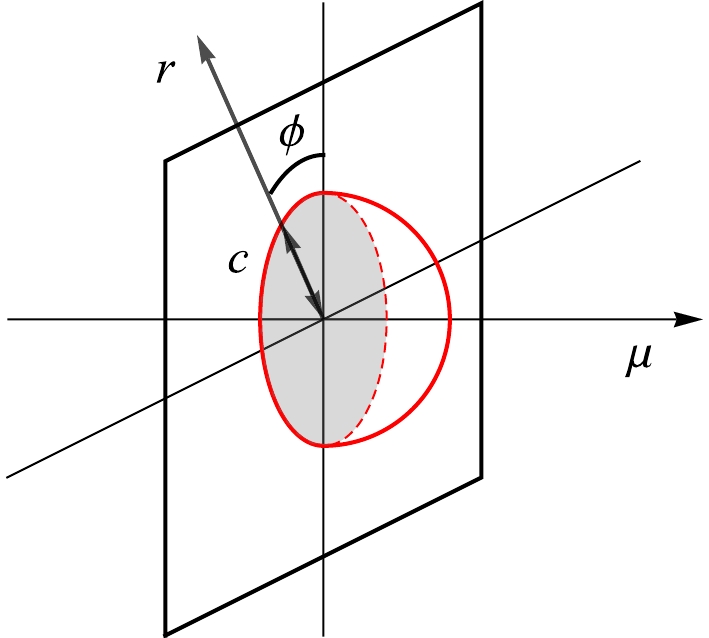
Figure 2. (color online) Minimal area as holographic entanglement entropy when the boundary metric is AdS.
$\begin{split} {\rm{Area}} =& 2\pi L \int_0^{r_0} {\rm d}r \cosh \left(\frac{\mu}{L}\right)\sinh \left(\frac{r}{\ell}\right)\\&\times\sqrt{\left(\frac{{\rm d}\mu}{{\rm d}r}\right)^2 + \left(\frac{L}{\ell}\right)^2\cosh^2\left(\frac{\mu}{L}\right)} . \end{split}$

(50) Through variation, one obtains a non-linear second-order differential equation for
$ \mu(r) $ , whose solution can be found owing to the embedding of$ {AdS}_4 $ inside$ {\mathbb R}^{2,3} $ (see Appendix B for extension to general dimensions).$ \tanh\left(\frac{\mu}{L}\right) = c \cosh \left(\frac{r}{\ell}\right), $

(51) where
$ 0<c<1 $ and otherwise it is an arbitrary constant. It is easy to see that the entanglement region is small (large) when$ c\sim 1 \,\,(c\sim 0) $ . Substituting the solution into the area (50) and introducing a cutoff$ \delta = (1- \tanh \left(\mu_{\max}/L\right))^{1/2} $ , one obtains$\begin{split} { \rm{Area}} =& 2\pi L^2\left(\frac{\sqrt{1- c^2} }{\sqrt{2}c }\frac{1}{\delta}-1-\frac{3 \sqrt{1-c^2} }{4 \sqrt{2} c }\delta-\frac{5 \sqrt{1-c^2} }{32 \sqrt{2} c }\delta ^3\right)\\&+{\cal O}\left(\delta ^4\right) .\\[-15pt] \end{split}$

(52) It is well known that the entanglement entropy follows perimeter law for conformal field theories, and we see that it is indeed the case here from the behavior of the divergent part (
$ \delta^{-1} $ ) for small entanglement region$ (c\sim 1) $ .Because we are going to expand around the explicit solution (51), it will be convenient to switch to new variables
$\begin{split} y =& \tanh\left(\frac{\mu}{L}\right), \\ x =& \cosh \left(\frac{r}{\ell}\right). \end{split}$

(53) Their range is by definition
$ x\geqslant 1 $ and$ |y| \leqslant 1 $ , and for the solution$ y = cx $ their range with the cutoff$ \delta $ becomes$ x\geqslant (1-\delta^2)/c, |y| \leqslant 1-\delta^2 $ . Our metric ansatz changes to$ \begin{split} {\rm d}s^2 =& {\rm d}\mu^2 + e^{2A} ({\rm d}r^2-\cosh^2 (r/\ell) {\rm d}t^2+ \ell^2 \sinh^2 (r / \ell) {\rm d}\phi ^2), \\ =& \frac{L^2}{(1-y^2)^2}{\rm d}y^2 +e^{2A}\left(\frac{\ell^2}{x^2-1}{\rm d}x^2-x^2 {\rm d}t^2 +\ell^2(x^2-1){\rm d}\phi^2 \right), \end{split} $

(54) while the area integral takes the following form.
$\begin{split} {\rm{Area }} =& 2\pi \ell L\int_1^{x_0} {\rm d}x \frac{e^{A}\sqrt{x^2-1}}{1-y^2} \sqrt{\left(y'\right)^2+\frac{\ell^2(1-y^2)^2}{L^2}\frac{e^{2A}}{x^2-1}}\\ \equiv &\int {\rm d}x {\cal L}(y,y'), \\[-15pt] \end{split}$

(55) where
$ (\bullet)': = \dfrac{{\rm d}(\bullet)}{{\rm d} x} $ in this section. For the AdS vacuum,$ e^{A} = (1-y^2)^{-1/2} $ . As we turn on scalar fields to consider Janus solutions, the metric function A changes, and so does$ y(x) $ , because of the change in the Euler-Lagrange equation. When we write$ {\cal L} = {\cal L}_{(0)} + {\cal L}_{(2)} \epsilon^2+\cdots $ and$ y = y_0 + y_2 \epsilon^2+ \cdots $ , using the fact that$ y_0 $ satisfies the minimal-area condition, we find$\begin{split} {\rm{Area}} =& \int^{x_0}_1 {\rm d}x\left( {\cal L} (y_0, y_0')+{\cal L} _{(2)} (y_0, y_0')\epsilon^2\right)\\&+ \left(\frac{\delta {\cal L}}{\delta y'}\right)_{(0)} y_2 \Big| _{x = 1}^{x = x_0}\epsilon^2+ {\cal O }(\epsilon^3), \end{split}$

(56) with cutoff
$ x_0 = (1-\delta^2)/c $ . The first term is$ {\cal O}(\epsilon^0) $ , and the answer is already given in (52), which exhibits linear divergence. In contrast, for$ y_n\, (n\geqslant 2) $ , we impose the boundary condition$ y_2(x = 1/c) = 0 $ to fix the boundary entangling region, and as the consequence we find that$ {\cal O}(\epsilon^2) $ and subsequent terms are consistently free from divergence, and starts with a finite term as$ \delta \rightarrow 0 $ .A comment is in order for the
$ SO(4)\times SO(4) $ case, where explicit solutions are available. The metric factor is here the same apart from a constant multiplication, i.e.,$ e^{A} = \sqrt{1-\epsilon^2}L/\ell \cosh(\mu/L) $ . It might seem innocuous, but in fact the metric is not AdS any more, and the changed Euler-Lagrange equation does not admit a simple solution like$ y = cx $ . We will first describe the minimal-area solutions collectively for all three models up to$ \epsilon^3 $ in our perturbative scheme below. For the$ SO(4)\times SO(4) $ case,$ \epsilon^3 $ -order correction is obviously absent, so we will discuss the$ \epsilon^4 $ -order calculation briefly after presenting general results.Let us now sketch the computation. We substitute the following expression into the minimal-area condition.
$ y(x) = c x\left(1+ \sum_{n = 2} \mathfrak{y}_n(x) \epsilon^n\right). $

(57) We find second order linear differential equations for
$ \mathfrak{y}_n $ . They generally assume the following form:$ \hat L \mathfrak{y}_n(x) = a_n F(x)+ H_n(x). $

(58) Namely, the homogeneous part is independent of n, the inhomogeneous part is written as the sum of n-independent and universal part
$ F(x) $ , and the remaining part$ H_n $ , which depends on n. The coefficients$ a_n $ are constant,$ a_2 = -\dfrac{k}{2} $ and$ a_3 = \dfrac{3}{2}{\tilde k} \cos 3 \zeta_* $ , where$ k = 1, 3, 7 $ and$ \tilde k = 0, 1, 7 $ for$ SO(4) \times SO(4) $ ,$ SU(3)\times U(1) \times U(1) $ and$ G_2 $ symmetric models. The differential operator$ \hat L $ and the universal part are in fact the same for all three models,$\begin{split} \hat L f =& \frac{\sqrt{1-c^2x^2}}{x^2(1-x^2)}\frac{{\rm d}}{{\rm d}x}\left(\frac{x^2 \left(1-x^2\right)}{\sqrt{1-c^2 x^2}}\frac{{\rm d}f}{{\rm d}x}\right), \\ F(x) =& \frac{2c \left(c^2 \left(x^2+1\right)-2\right)}{\left(x^2-1\right) \left(c^2 x^2-1\right)} . \end{split} $

(59) The model-dependent parts
$ H_n $ for$ n = 2,3 $ are given as$ \begin{split} H_2(x) =& 0 , \\ H_3(x) =& \tilde{k}\Big[\frac{c \left(8 c^6 x^4 \left(3 x^2\!\!-\!\!5\right)\!-\!\!24 c^4 x^2 \left(x^2\!\!-\!\!3\right)\!-\!\!c^2 \left(17 x^2\!\!+\!\!33\right)\!\!+\!\!18\right)}{3 \left(x^2-1\right) \left(c^2 x^2-1\right)}\\&\times\cos(3\zeta_*) \! +\!\frac{4 \left(c^4 x^2 \left(3 x^2\!-\!1\right)\!-\!3 c^2 \left(x^2\!-\!1\right)\!-\!2\right)}{3 x \left(x^2-1\right) \left(c^2 x^2-1\right)}\sin( 3 \zeta_*) \\ &\!+\!\frac{4 \left(2 c^4 x^2 \left(3 x^2\!\!-\!\!5\right)\!\!+\!\!3 c^2 \left(x^2\!\!+\!\!1\right)\!-\!\!2\right)}{3 x \left(x^2-1\right)}\sqrt{1\!\!-\!\!c^2 x^2} \sin( 3 \zeta_*) \Big] . \end{split} $

(60) Readers might wonder why the inhomogeneous part, i.e., the right-hand-side of (58) takes similar forms for different models. This is because the warp factor
$ e^A $ takes the following universal form, at least up to$ \epsilon^3 $ .$ e^{A} = \frac{L}{l \sqrt{1-y^2}}\left(1-\frac{k}{2}\epsilon^2+\tilde{k}{\mathscr A}_3\epsilon ^3+{\cal O }(\epsilon^4)\right), $

(61) where
$ k = 1, 3, 7 $ and$ \tilde{k} = 0, 1, 7 $ for$ SO(4) \times SO(4) $ ,$ SU(3)\times U(1) \times U(1) $ and$ G_2 $ , respectively, and$ {\mathscr{A}}_3 = \frac{2}{3} \left(2y(1-( 1-y^2)^\frac{3}{2} )\sin 3 \zeta_*+ (3-3y^2+2y^4)\cos 3 \zeta_* \right). $

(62) They start to differ at
$ \epsilon^4 $ , but for simplicity we consider the minimal surface only up to$ \epsilon^3 $ here. For$ SO(4)\times SO(4) $ ,$ {\mathscr{A}}_3 = 0 $ , and$ {\mathscr{A}}_4 $ is constant, and we discuss the$ \epsilon^4 $ -order solution separately later.It is evident from the form of
$ \hat L $ that Eq. (58) can be treated as a first order differential equation for$ \mathfrak{y}_n $ . Owing to the linearity, the solutions generally take the following form,$ \mathfrak{y}_n(x) = \mathfrak{y}^{(h)} (x) + a_n \mathfrak{y}^{(u)} (x) +\mathfrak{y}_n ^{(m)}(x), $

(63) where
$ \mathfrak{y}^{(h)} $ is the homogeneous solution, and$ \mathfrak{y}^{(u)},\mathfrak{y}^{(m)}_n $ are particular solutions for$ F, H_n $ respectively. Homogeneous solutions are easily found,$ \mathfrak{y}^{(h)}(x) = c_1 \left(-\frac{\sqrt{1-c^2 x^2}}{x} + \sqrt{1-c^2} \sinh^{-1} \left( \frac{\sqrt{c^2-1} x}{\sqrt{x^2-1}}\right) \right) + c_2. $

(64) We note that the part with
$ c_1 $ is divergent at$ x = 1 $ . Without losing generality, we can choose$ \mathfrak{y}^{(h)}(x) = 0 $ in (63), since it can be included in the in-homogeneous solutions. We then need to construct particular solutions$ \mathfrak{y}^{(u)},\mathfrak{y}^{(m)}_n $ and impose$ \mathfrak{y}(1/c) = 0 $ and regularity at$ x = 1 $ .Now, let us turn to the inhomogeneous part.
$ {\rm d}(\mathfrak{y}^{(u)})/{\rm d}x $ , the first derivate of an inhomogeneous solution for$ F(x) $ , is given as$\begin{split} \frac{{\rm d}\mathfrak{y}^{(u)}}{{\rm d}x} =& \frac{ c^2 \left(x^2-2\right)+1}{c x \left(x^2-1\right)}\\&-\frac{ \sqrt{1-c^2 x^2} \left(c \sqrt{1-c^2}+\left(1-2 c^2\right)( \sin ^{-1}c x- \sin ^{-1}c)\right)}{c^2 x^2 \left(x^2-1\right)}. \end{split} $

(65) Unfortunately its integration cannot be done analytically, and we have instead
$\begin{split} \label{yuni} \mathfrak{y}^{(u)}(x) =& \mathfrak{y}^{(u)}_* - \frac{\sqrt{1-c^2} \sqrt{1-c^2 x^2}}{c x}+ \frac{1-c^2}{c} \log \left( \sqrt{1-c^2x^2} + \sqrt{1-c^2} x \right) -\frac{1-2c^2}{c} \log x -\frac{1-2 c^2} {c^2 x (x^2-1) } \left(\sin^{-1}c - \sin^{-1} cx \right) \\ &\times \left( \sqrt{1-c^2x^2} + c x \sin ^{-1} cx \right)-\int_{1/c}^x {\rm d}x' \frac{(1-2c^2)(\sqrt{1-c^2 x'^2} + cx' \sin^{-1} c x' )} {c^2 x' (x'^2 -1) ^2 } \left(\frac{c (x'^2-1)}{\sqrt{1-c^2x'^2}} + 2 x' (\sin^{-1} c - \sin^{-1} c x' ) \right) , \end{split} $

(66) which is finite at
$ x = 1 $ , and the integration constant$ \mathfrak{y}^{(u)}_* $ is chosen to guarantee$ \mathfrak{y}^{(u)}(1/c) = 0 $ .$\begin{split} \mathfrak{y}^{(u)}_* =& {c} \log c- \frac{1-c^2}{2c} \log \left( {1-c^2}\right) \\&+ \frac{\pi c (1-2c^2) ( \pi - 2 \sin^{-1} c ) }{4 (c^2-1)}. \end{split}$

(67) The particular solution due to
$ H_3 $ can be also obtained in the same fashion. Let us just present the result here.$ \mathfrak{y}_3^{(m)} = \tilde{k}\left[\frac{3}{2} \cos 3 \zeta_* \ \mathfrak{y}^{(u)}(x) + S(x) \sin3 \zeta_*+ C(x) \cos3 \zeta_* \right], $

(68) $\begin{split} S(x) =& c ( 1-c^2)^2( 2\sin ^{-1}(c x)- \pi) -\frac{4}{3 x}\left( 1- c^2 x^2\right) \\ &+\sqrt{1-c^2 x^2} \left(\frac{c^2}{3} \left(c^2 x^3-3 c^2 x+x\right)\right.\\&\left.+\frac{6c^4- 9 c^2 +4}{3 x}\right), \end{split} $

(69) $ \begin{split} C(x) =& \frac{1}{6 x}c \left(2 c^4 x^5-12 \left(1-c^2\right)^{3/2} \sqrt{1-c^2 x^2}+\left(6 c^2-3\right) x\right.\\&+\left(c^2-6 c^4\right) x^3\bigg) -c \left(1-c^2\right)^2 \left(2 \log \left(\sqrt{1-c^2} x\right.\right.\\&\left.\left.-\sqrt{1-c^2 x^2}\right)-\log \left(1-c^2\right)+2 \log (c)\right). \end{split} $

(70) One can plot the minimal area surface for pure AdS and Janus solutions, as shown in Fig. 3. Intuitively, the minimal surface must be pushed away from the center of AdS due to the redshift effect when there is nontrivial excitation.

Figure 3. Minimal area surfaces. Left panel depicts AdS vacuum, and right panel depicts nontrivial Janus backgrounds.
We now substitute these solutions into (56) and evaluate up to
$ \epsilon^3 $ terms,$ {\rm{Area}} = {\rm{Area}} _{(0)} + {\rm{Area}} _{(2)} \epsilon^2 + {\rm{Area}} _{(3)} \epsilon^3 + {\cal O} (\epsilon^4). $

(71) The leading terms of the integral in the limit of
$ \delta\rightarrow 0 $ can be evaluated using the differential equation for$ \mathfrak{y}_n $ . The results are$\begin{split} {\rm{Area}} _{(2)} =& \pi L^2 k\left(\frac{ \left(2 c \sqrt{1-c^2} +(\pi-2) \left(c^2-2\right) \sin ^{-1}c \right)}{3 c \sqrt{1-c^2} }\right.\\&\left.+\frac{\sqrt{2-2 c^2} }{c }\delta\right)+{\cal O}\left(\delta ^2\right) , \end{split}$

(72) $ \begin{split} &{\rm{Area}}_{(3)} = 2\pi L^2 \tilde{k}\\&\quad\times \left[\left(\frac{2 \left(c^4\!+\!c^2\!-\!2\right) \sqrt{1\!-\!c^2} }{3 c}\!+\!\frac{4 \left(2 c^4\!+\!c^2\!+\!12\right) \sqrt{1\!-\!c^2} }{15 c}\delta ^2\right) \sin3 \zeta_*\right. \\ &\quad \left.+\left(\frac{1}{3} \left(1-c^2\right) \left(2 c^2-3\right) +\frac{3 \sqrt{1-c^2} }{\sqrt{2} c}\delta-\frac{8}{15} c^4 \delta ^2\right)\cos3\zeta_*\right] \\ & \quad-3\frac{\tilde{k}}{k} \cos 3 \zeta_* \ {\rm{Area}} _{(2)}+{\cal O}\left(\delta ^3\right). \end{split} $

(73) Now let us turn to the case of
$ SO(4)\times SO(4) $ , where the$ \epsilon^3 $ -order correction is absent. Let us stress again that although the warp factor changes only by a numerical factor, the minimal area surface and the associated holographic entanglement entropy is non-trivial. At$ \epsilon^2 $ , we managed to obtain analytic results. One can easily continue the analysis of the surface-area action in the manner of (56) and find that$ {\hat L }\mathfrak{y}_4(x) = -\frac{1}{8} F(x) + H_4(x), $

(74) $\begin{split} &H_4(x) =\\&\quad \frac{2 c x \mathfrak{y}_2'(x) \left(x \left(c^2 x^2-1\right) \mathfrak{y}_2'(x)-\mathfrak{y}_2(x)\right)}{\left(c^2 x^2-1\right)^2}+\frac{c \left(c^2 \left(5 x^2-3\right)-2\right)}{4\left(x^2-1\right) \left(c^2 x^2-1\right)} \\ &\quad- \left(\frac{ \left(c^4 \left(x^4+x^2\right)-c^2 \left(x^2+3\right)+2\right) }{\left(x^2-1\right) \left(c^2 x^2-1\right)^2}\mathfrak{y}_2(x)+ \frac{3c^2 x }{1-c^2 x^2} \mathfrak{y}_2'(x)\right), \end{split} $

(75) where
$ \mathfrak{y}_2 = \mathfrak{y}^{(u)} $ in (66). One should then integrate the differential equation above, however this unfortunately does not seem feasible due to the sophisticated inhomogeneous part in$ H_4 $ . -
In this study, we applied a perturbative technique, where we expand the supergravity equations around a pure AdS configuration in an expansion parameter, which is one of the integration constants, and solve the linearized equations order-by-order iteratively. We have intended to be illustrative, and considered three simple models that are consistent truncations of
$ D = 4, $ $SO(8) $ gauged supergravity and have studied Janus solutions. Let us stress here that our method is different from the conventional series expansion of the field equations near UV (i.e., near the boundary of AdS), where the IR boundary condition cannot be incorporated analytically and one usually has to rely on numerical integration. In our method, we instead impose the IR boundary condition at every order in$ \epsilon $ , and the holographically renormalized quantities can be obtained exactly as a function of CFT deformation parameters. Although we have considered only single-scalar models in this paper, the advantage of our method stands out more strongly when we consider multi-scalar models (e.g., Ref. [24]), where thorough numerical analysis is significantly more time-consuming.There are evidently several avenues to investigate further. One is to study other supergravity models. There are numerous studies on supersymmetric Janus solutions in various dimensions [6, 8-22], and one can obviously apply our method and construct the solutions in a semi-analytic form.
It will be also worthwhile to attempt to extract other physical quantities from Janus configurations, such that one can eventually compare with the corresponding field theory side computations. We note that in Ref. [41], single-scalar models were studied using a first-order formalism, inspired by the Hamilton-Jacobi theory, and then the result was used to calculate holographic entanglement entropy and boundary OPE. We also note that the contribution of the interface to the correlation functions and sphere partition functions are discussed in Ref. [42], where the solutions connect two different conformal fixed points. Perhaps from a more fundamental perspective, one would like to identify the conformal field theory living on the interface, namely the conformal field theory dual of the
$ {AdS}_3 $ slice in our setting, from the holographic results of correlation functions, partition function, and entanglement entropy. Ref. [43], for example, provides a discussion of how marginal deformation affects the partition function when the spacetime has a boundary (interface) from the calculations in free field theory.Let us also point out an interesting generalization of Janus configurations in the literature. One can consider space-modulated deformations, and with an ingenious choice of the ansatz, one still obtains ordinary differential equations [44], allowing analytic control, while in the most general setup one has to solve partial differential equations. An interesting physical consequence is so-called boomerang RG [45,46], namely analogues of c-theorem can be avoided, and the same conformal field theory can be encountered at both ends of the renormalization group. Let us add that for the ABJM model, spatially modulated mass deformations were studied both holographically and on the field theory side in a number of papers [47–51]. One can certainly re-visit the holography-side analysis employing our method and also study spatially modulated solutions in other AdS/CFT examples. We plan to report on these topics in the near future.
-
In this appendix, we present the BPS equations and their solutions obtained using our perturbative prescription for the
$ G_2 $ symmetric model. In terms of the superpotential, the BPS equation is given as$\tag{A1} \alpha' = -\frac{1}{14} \left(\frac{A'}{W^2}\right)\frac{\partial W^2}{\partial \alpha}- \left(\frac{e^{-A}}{7\ell}\right) \frac{1}{\sinh (2 \alpha)}\frac{1}{W^2} \frac{\partial W ^2} {\partial \zeta}, $

(A1) $\tag{A2} \zeta' = -\frac{2}{7} \left(\frac{A'}{W^2}\right)\frac{1}{\sinh^2 (2\alpha)}\frac{\partial W^2}{\partial \zeta}+\left(\frac{e^{-A}}{7\ell}\right) \frac{1}{\sinh (2 \alpha)}\frac{1}{W^2} \frac{\partial W^2 } {\partial \alpha}. $

(A2) More concretely, one obtains
$\tag{A3} \begin{split} \alpha' =& -\frac{1}{64} \left(\frac{A'}{W^2}\right) \sinh 2 \alpha \left(\sinh 2 \alpha \cos \zeta +\cosh 2 \alpha \right)^2 \left(-2 \sinh 4 \alpha \left(4 \sinh 4 \alpha \cos 4 \zeta\right.\right.\\&\left.\left. +25 \cos \zeta -14 \cos 3 \zeta \right) +\sinh 8 \alpha \left(10 \cos 3 \zeta -7 \cos \zeta \right)\right. \\ & \left. +8 \sinh ^3 2 \alpha \left(\cosh 2 \alpha \cos 5 \zeta -6 \sinh 2 \alpha \cos 2 \zeta \right)+8 \cosh 4 \alpha +14 \cosh 8 \alpha +42 \right) \\&+ \left(\frac{e^{-A}}{8\ell}\right) \frac{1}{\sinh 2 \alpha}\frac{1}{W^2} \sinh ^3 2 \alpha \sin \zeta \left(\sinh 2 \alpha \cos \zeta+\cosh 2 \alpha \right)^2\\& \times \left(2 \sinh ^2 2 \alpha \cos 4 \zeta -4 \sinh 4 \alpha \left(4 \cos \zeta +\cos 3 \zeta \right)+\cosh 4 \alpha \left(11 \cos 2 \zeta +10\right)+13 \cos 2 \zeta +2\right), \end{split} $

(A3) $\tag{A4} \begin{split} \zeta' = &\frac{1}{4} \left(\frac{A'}{W^2}\right)\frac{1}{\sinh^2 2\alpha} \sinh ^3 2 \alpha \sin \zeta \left(\sinh 2 \alpha \cos \zeta+\cosh 2 \alpha \right)^2 \left(2 \sinh ^2 2 \alpha \cos 4 \zeta -4 \sinh 4 \alpha \left(4 \cos \zeta +\cos 3 \zeta \right)\right.\\&\left.+\cosh 4 \alpha \left(11 \cos 2 \zeta +10\right)+13 \cos 2 \zeta +2\right) +\left(\frac{e^{-A}}{32 \ell}\right) \frac{1}{\sinh 2 \alpha}\frac{1}{W^2} \sinh 2 \alpha \left(\sinh 2 \alpha \cos \zeta +\cosh 2 \alpha \right)^2 \\&\times \left(-2 \sinh 4 \alpha \left(4 \sinh 4 \alpha \cos 4 \zeta +25 \cos \zeta -14 \cos 3 \zeta \right) +\sinh 8 \alpha \left(10 \cos 3 \zeta -7 \cos \zeta \right)\right. \\& \left. +8 \sinh ^3 2 \alpha \left(\cosh 2 \alpha \cos 5 \zeta -6 \sinh 2 \alpha \cos 2 \zeta \right)+8 \cosh 4 \alpha +14 \cosh 8 \alpha +42 \right), \end{split} $

(A4) The real superpotential is given as follows.
$\tag{A5} \begin{split} W^2 = &2 \cosh ^{14}\alpha \Big(14 \tanh ^{11}\alpha \cos 3 \zeta +14 \tanh ^{10}\alpha \cos 4 \zeta +2 \tanh ^7\alpha (49 \cos \zeta +\cos 7 \zeta ) +14 \tanh ^4\alpha \cos 4 \zeta \\&+14 \tanh ^3\alpha \cos 3 \zeta +\tanh ^{14}\alpha +49 \tanh ^8\alpha +49 \tanh ^6\alpha+1\Big). \end{split} $

(A5) The third order solutions are
$\tag{A6} \begin{split} \alpha_3 (\mu) =& \frac{1}{24} {\rm{sech}}^2\left(\frac{\mu}{L}\right) \left[3 {\rm{sech}}^2\left(\frac{\mu}{L}\right) \left(32 \sinh \left(\frac{\mu}{L}\right) \sin 4 \zeta_*\right.\right.+9 \left(\sinh \left(\frac{\mu}{L}\right)-3 \sinh \left(\frac{3\mu}{L}\right)\right) \sin 6 \zeta_* \\& \left. \left.+8 \left(\cosh \left(\frac{2\mu}{L}\right)-3\right) \cos 4 \zeta_*+9 \left(7 \cosh \left(\frac{2\mu}{L}\right)+3\right) \cos 6 \zeta_*\right)-58\right], \end{split} $

(A6) $\tag{A7}\begin{split} \zeta_3(\mu) = &9 {\rm{sech}}\left(\frac{\mu}{L}\right) \left(12 \tanh \left(\frac{\mu}{L}\right) \sin 3 \zeta_*+\left(5 \cosh \left(\frac{2 \mu}{L}\right)-7\right) {\rm{sech}}\left(\frac{\mu}{L}\right) \cos 3 \zeta_*\right)\tan ^{-1}e^{\frac{\mu}{L}} +3 \left(2 {\rm{sech}}^4\left(\frac{\mu}{L}\right)-7 {\rm{sech}}^2\left(\frac{\mu}{L}\right)+5\right)\sin\zeta_* \\ & +\frac{1}{24} \left({\rm{sech}}\left(\frac{\mu}{L}\right) \left(736 {\rm{sech}}^3\left(\frac{\mu}{L}\right)-9 \left(72 \pi \sinh \left(\frac{\mu}{L}\right)+71\right) {\rm{sech}}\left(\frac{\mu}{L}\right)+224\right)-321\right)\sin3 \zeta_* +3 \left(8 {\rm{sech}}^6\left(\frac{\mu}{L}\right)-14 {\rm{sech}}^4\left(\frac{\mu}{L}\right)\right. \\ & \left. +{\rm{sech}}^2\left(\frac{\mu}{L}\right)+5\right)\sin7 \zeta_* -\frac{9}{64} \left(35 (\cosh \left(\frac{4\mu}{L}\right)+3)-116 \cosh \left(\frac{2\mu}{L}\right)\right) \tanh ^2\left(\frac{\mu}{L}\right) {\rm{sech}}^4\left(\frac{\mu}{L}\right)\sin9\zeta_* \\ & +\left(\frac{15 \pi }{2}-6 \tanh ^3\left(\frac{\mu}{L}\right) {\rm{sech}}\left(\frac{\mu}{L}\right)-30\tan ^{-1}e^{\frac{\mu}{L}}\right)\cos \zeta_* +\left(\frac{9\pi}{2} \left(6 {\rm{sech}}^2\left(\frac{\mu}{L}\right)-5\right)+\frac{1}{24} \tanh \left(\frac{\mu}{L}\right) {\rm{sech}}\left(\frac{\mu}{L}\right)\right.\\&\times \left. \left(736 {\rm{sech}}^2\left(\frac{\mu}{L}\right)-397\right)\right)\cos3\zeta_* +3 \tanh \left(\frac{\mu}{L}\right) {\rm{sech}}\left(\frac{\mu}{L}\right) \left(8 {\rm{sech}}^4\left(\frac{\mu}{L}\right)-10 {\rm{sech}}^2\left(\frac{\mu}{L}\right)-3\right)\cos7 \zeta_* \\ & +\frac{9}{8} \tanh \left(\frac{\mu}{L}\right) {\rm{sech}}\left(\frac{\mu}{L}\right) \left(32 {\rm{sech}}^4\left(\frac{\mu}{L}\right)-80 {\rm{sech}}^2\left(\frac{\mu}{L}\right)+63\right)\cos9\zeta_*, \end{split} $

(A7) $\tag{A8} {\cal A}_3(\mu) = -\frac{28}{3} \tanh\left(\frac{\mu}{L}\right) \left({\rm{sech}}^3\left(\frac{\mu}{L}\right)-1\right)\sin3 \zeta_* +\frac{7}{6} \left(2 \cosh \left(\frac{2 \mu}{L}\right)+\cosh \left(\frac{4 \mu}{L}\right)+9 \right) {\rm{sech}}^4\left(\frac{\mu}{L}\right)\cos3\zeta_*. $

(A8) -
We present here the minimal area surface solutions inside the AdS spacetime of general dimensionality. In global coordinates, the metric of round AdS
$ {}_{d+1} $ can be written as$\tag{B1} {\rm d}s^2 = \frac{L^2}{\cos^2 \xi } \left(-{\rm d}t^2 +{\rm d}\xi^2 + \sin^2 \xi \, {\rm d}\Omega^2_{d-1}\right), $

(B1) where
$ {\rm d}\Omega_{d-1}^2 $ denotes the$ (d-1) $ -dimension sphere with unit radius. This can be derived as induced metric on the surface defined by$\tag{B2} \sum\limits_{i = 1}^d (X^i)^2 -(X^{d+1})^2-(X^{d+2})^2 = -L^2, $

(B2) inside
$ {\mathbb R}^{d,2} $ with natural flat metric. An explicit parametrization that leads to (B1) is$\tag{B3} \begin{split} X^i =& L\tan \xi \,Y^i , \\ X^{d+1} = &L\sec \xi \sin t , \\ X^{d+2} =& L\sec \xi \cos t, \end{split} $

(B3) where
$ Y^i $ defines the spatial part of the boundary$ S^{d-1} $ , i.e.$ \sum_i (Y^i)^2 = 1 $ . The definition (B2) is also useful to derive the relation$ {\rm d}s^2_{AdS_{d+1}} = {\rm d}\mu^2+\cosh^2\mu \, {\rm d}s^2_{AdS_{d}} $ : one can attempt$ X^1 = \sinh\mu $ and$ X^i = \cosh\mu {\tilde X}^i \,\, (i = 2,\cdots, d+2) $ and make$ {\tilde X}^{i}\,\, (i = 2,\cdots, d+2) $ define$ AdS_{d} $ . We also note that an alternative representation of AdS in global coordinates,$\tag{B4} {\rm d}s^2 = {\rm d}\rho^2 - \cosh^2\rho \, {\rm d}t^2 + \sinh^2\rho \,{\rm d}\Omega^2_{d-1}, $

(B4) is related to (B1) simply through
$ \sec \xi = \cosh\rho $ , or equivalently$ \tan \xi = \sinh\rho $ .Now let us consider the holographic entanglement entropy as the minimal surface area inside bulk AdS [32]. We can write
$ {\rm d}\Omega^2_{d-1} = {\rm d}\theta^2+\sin^2\theta {\rm d}\Omega_{d-2} $ , and for simplicity, we choose to divide the boundary into two parts, separated by a constant latitude curve$ \theta = \theta_0 $ . In terms of$ \xi(\theta) $ , which describes the shape of the surface in the bulk, the area is$\tag{B5} {\rm{Area}} = L^{d-1} {\rm vol} (S^{d-2}) \int_0^{\theta_0} {\rm d}\theta \frac{(\sin \xi \sin \theta)^{d-2}}{\cos^{d-1}\xi} \sqrt{\left( \frac{{\rm d}\xi}{{\rm d}\theta}\right)^2 +\sin^2 \xi} . $

(B5) One can check that the following relation satisfies the Euler-Lagrangian equation derived from Eq. (B5), for constant c.
$\tag{B6} \cos \theta \sin \xi = c. \label{min_area_sol} $

(B6) Evidently, this equation is equivalent to (51), when we identify
$ \sec\xi = \cosh(\mu/L)\cosh(r/\ell),\quad \tan\xi\cos\theta = \sinh(\mu/L). $

From the above parametrization, it is easy to see that this curve is equivalent to the following quadratic equation
$\tag{B7} c^{-2}(X^1)^2 - (X^{d+1})^2 - (X^{d+2})^2 = 0 . $

(B7) Or, as we consider spatial surfaces at a given time defined by
$ X^{d+1}-\tan t X^{d+2} = 0 $ , (B6) is an intersection with a plane$ X^1 \sin t = c X^{d+1} $ .It is now straightforward to substitute the solution (B6) into the integral (B5), and calculate the area. The result for general dimensions is provided, e.g., in Ref. [40].
Re-visiting supersymmetric Janus solutions: a perturbative construction
- Received Date: 2020-01-24
- Available Online: 2020-07-01
Abstract: We construct holographic Janus solutions, which describe a conformal interface in the theory of M2-branes, in four-dimensional gauged supergravities using a perturbative method. In particular, we study three Einstein-scalar systems and their BPS equations, which are derived by Bobev, Pilch, and Warner (2014). The actions of our interest are all consistent truncations of


 DownLoad: