


 Abstract
 HTML
HTML Reference
 Related
 PDF
PDF


-
In general relativity, the standard quantum field theory (QFT) based on perturbations and renormalization procedures focuses mainly on the loop effects, expectation values or equal-time correlations in space-times of interest for cosmology such as, for example, de Sitter expanding universe, which was intensively studied [1–10]. An alternative approach are the non-perturbative methods based on the Bogolyubov transformations for analyzing the cosmological particle creation, which avoid the difficulties of perturbative QFT [11–18]. Even though these two approaches involve different mechanisms, they are compatible and complete each other in constructing plausible inflationary scenarios.
The central element in these investigations are the spatially flat FLRW manifolds, which are somewhat equivalent as long as they allow conformally transformed Minkowskian charts. In these charts, the massless fields satisfying the conformal covariant field equations behave in a similar manner. However, the presence of massive fields breaks the conformal symmetry such that in each space-time of this type we have a different QFT whose specific processes need to be studied.
An advantage of these manifolds is that they are symmetric under translations and, as a consequence, there exist quantum modes which are expressed in terms of plane waves with similar properties, as in special relativity. For this reason, these manifolds are useful for studying the behavior of quantum matter in the presence of classical gravity by considering the perturbation methods in QFT, in which significant results were obtained by many authors who considered the simpler case of first order perturbations without loop corrections [19–26].
These processes are of a special interest since they are forbidden in the Minkowski space-time, since the energy and momentum cannot be conserved simultaneously in the Feynman diagrams with three external lines. However, this restriction does not hold in the FLRW manifolds, where in general the energy is no longer conserved. Moreover, in de Sitter space-time, where the energy is conserved, the energy operator does not commute with momentum so that the energy and momentum cannot be conserved simultaneously, meaning that their measurement is affected by an uncertainity [19–21, 27–29].
Inspired by these results, we built a QED in the Coulomb gauge in de Sitter expanding universe [29], and analyzed many processes in the first order perturbations [29–31]. Recently, we completed this approach with an integral representation of the fermion propagators that are needed for calculating the Feynman diagrams of any order [32] without resorting to the laborious Schwinger-Keldysh method [33–35] used so far. Thus, we have a good example of a complete QED in a curved background, which remains, however, the only example of this type so far.
Looking for another example of a manifold where QED could be constructed without huge difficulties, we observed that an expanding space-time exists where the equations for the massive free fields can be solved analytically [36]. This is the
$ (1+3) $ -dimensional spatially flat FRLW manifold, whose expansion is given by a Milne-type scale factor proportional to the proper (or cosmic) time t. This space-time is interesting and somewhat special since it is generated by gravitational sources behaving as$ \frac{1}{t^2} $ , in contrast to the genuine Milne universe which is flat and has no gravitational sources [37].However, the major advantage of this geometry is that it hosts a friendly QED which can be constructed with the help of the Lehmann-Symanzik-Zdoiermann (LSZ) reduction formalism [38–40] in a similar manner as in de Sitter space-time [29], but giving different or even complementary results. For example, the solutions of the free Dirac equation are similar to those in de Sitter space-time but with the mass and momentum that are interchanged. Thus, our Milne-type spatially flat FLRW space-time is interesting and helpful in investigating the technical features of a QED in a curved background, regardless of the speculations concerning the physical interpretation of the singularity at
$ t = 0 $ .Encouraged by these arguments, we investigate here the QED processes in the first order perturbations, derive their amplitudes and study the resulting probabilities and rates. Our approach respects ad litteram the quantum principles, and assumes that the quantum states are prepared or measured by a global apparatus represented by an algebra of observables. Among them are the conserved observables, which are just the Killing vector fields of the background that are defined globally. Hence, we can prepare global quantum modes independent of the local charts, and choose the eigenvectors of a system of commuting operators and their eigenvalues, which are the conserved quantities, to label the quantum modes. In this framework, we can perform the canonical quantization of the interacting fields of QED in the Coulomb gauge as in Ref. [29], and then introduce the LSZ reduction formalism to derive the amplitudes of the allowed processes in the first order perturbations.
In the new QED, we must re-define the transition rates, since the Dirac δ-function for energy conservation is replaced by a different time integral. By doing so, we obtain plausible transition rates, which have the well-known problems of the perturbation theory, namely the infrared divergence due to the massless photon, and a divergence that appears in some particular direction when studying angular dependence. The first cannot be solved at this level before analysing the concrete infrared regulators (e.g. associations of processes which cancel the divergence). However, the angular divergences can be removed at any time and the physical results extracted by following the method of reduced amplitudes proposed by Yennie et al [41], which was used successfully in other investigations [42–44]. Thus, we can obtain the angular dependence of the transition rates and analyze them using graphical methods. We note that this is the first time an angular analysis is carried out in the FLRW manifold. There are serious technical difficulties which discouraged us to perform a similar study in de Sitter QED.
We begin in Sec. 2 by defining the Milne-type spatially flat FRLW space-time, and by deriving the fundamental solutions of the free Dirac and Maxwell fields in this manifold. In the next section, we outline a QED in this space-time and use the LSZ formalism to derive the first order amplitudes of the principal processes. In Sec. 4, we propose a new definition of the transition rate that can be applied in the case the energy is not conserved. We find that the probability of transitions between charged states vanishes, and that only the transitions between neutral states remain. Their properties are studied in Sec. 5 by resorting to graphical methods. Finally, we present our concluding remarks.
-
Let us start with the
$ (1+3) $ -dimensional spatially flat FLRW manifold M with the scale factor$ a(t) = \omega t $ , where$ t\in (0,\infty) $ is the proper (or cosmic) time of the usual FLRW chart whose coordinates$ x^{\mu} $ (labeled by the natural indices$ \alpha,...\mu,... = 0, 1, 2, 3 $ ) are$ x^0 = t $ and the Cartesian space coordinates,$ x^i $ ($ i,j,k... = 1,2,3 $ ), for which we use the vector notation$ \vec{x} = (x^1,x^2,x^3) $ . This chart, denoted by$ \{t,\vec{x}\} $ , is related to the conformal flat chart$ \{t_c,\vec{x}\} $ , where we have the same space coordinates but the conformal time$ t_c\in (-\infty,\infty) $ is defined as$ t_c = \int \frac{{\rm d}t}{a(t)} = \frac{1}{\omega} \ln(\omega t) \; \to\; a(t_c)\equiv a[t(t_c)] = {e}^{\omega t_c}\,. $

(1) The corresponding line element reads
$ \begin{split} {\rm d}s^2 =& g_{\mu\nu}(x){\rm d}x^{\mu}{\rm d}x^{\nu} = {\rm d}t^2-(\omega t)^2 {\rm d}{\vec x}\cdot {\rm d}{\vec x}\\ =& {e}^{2\omega t_c}({\rm d}t_c^2-{\rm d}{\vec x}\cdot {\rm d}{\vec x})\,. \end{split}$

(2) Note that the constant ω, introduced from dimensional considerations, is a useful free parameter representing the speed of expansion of M. We recall that in the case of the genuine Milne universe (with negative space curvature, but globally flat), one must set
$ \omega = 1 $ to eliminate the gravitational sources [37].In contrast, our space-time M is produced by isotropic gravitational sources, i.e. the density ρ and pressure p evolve with time as
$ \rho = \frac{3}{8\pi G}\frac{1}{t^2}\,, \quad p = -\frac{1}{8\pi G}\frac{1}{t^2}\,, $

(3) and vanish for
$ t\to\infty $ . These sources govern the expansion of M that can be better observed in the chart$ \{t, \vec{\hat x}\} $ of 'physical' space coordinates$ \hat x^i = \omega t x^i $ , where the line element$ {\rm d}s^2 = \left(1-\frac{1}{t^2}\vec{\hat x}\cdot \vec{\hat x}\right){\rm d}t^2 + 2 \vec{\hat x}\cdot {\rm d}\vec{\hat x}\,\frac{{\rm d}t}{t}-{\rm d}\vec{\hat x}\cdot {\rm d}\vec{\hat x}\,, $

(4) corresponds to an expanding horizon at
$ |\vec{\hat x}| = t $ , and tends to the Minkowski space-time for$ t\to \infty $ and for vanishing gravitational sources.In what follows we consider only the FLRW and conformal charts where we introduce the local orthogonal non-holonomic frames defined by the vector fields
$ e_{\hat\alpha} = e_{\hat\alpha}^{\mu}\partial_{\mu} $ , labeled by the local indices$ \hat\mu,\hat\nu,... = 0,1,2,3 $ , and the associated co-frames given by the 1-form$ \omega^{\hat\alpha} = \hat e_{\mu}^{\hat\alpha}dx^{\mu} $ . In a given tetrad gauge, the metric tensor is expressed as$ g_{\mu\nu} = \eta_{\hat\alpha\hat\beta}\hat e^{\hat\alpha}_{\mu}\hat e^{\hat\beta}_{\nu} $ , where$ \eta = {\rm diag}(1,-1,-1,-1) $ is the Minkowski metric. Here, we are interested in choosing the tertrad gauge which preserves the global symmetry of M. Bearing in mind that M has the isometry group$ E(3) = T(3)\circledS SO(3) $ (of space translations and rotations), this can be done only by using the Cartesian space coordinates and the diagonal tetrad gauge,$ e_0 = \partial_t = e^{-\omega t_c}\,\partial_{t_c}\,,\quad \omega^0 = {\rm d}t = e^{\omega t_c}{\rm d}t_c\,, $

(5) $ e_i = \frac{1}{\omega t}\,\partial_i = e^{-\omega t_c}\,\partial_i\,, \quad \omega^i = \omega t {\rm d}x^i = e^{\omega t_c}{\rm d}x^i\,, $

(6) which we need to write the Dirac equation.
For calculating the Feynman diagrams, we must have the quantum modes of the free fields in M. Let us start with the massive Dirac field ψ of mass m which satisfies the field equation
$ (E_D-m)\psi = 0 $ , where$ E_D = i\gamma^0\partial_{t}+i\frac{1}{\omega t}\gamma^i\partial_i +\frac{3i}{2}\frac{1}{t}\gamma^{0}-m\,. $

(7) The term of this operator depending on the Hubble function
$ \frac{\dot{a}}{a} = \frac{1}{t} $ can be removed at any point by substituting$ \psi \to (\omega t)^{-\frac{3}{2}}\psi $ .The fundamental solutions of the Dirac equation can be defined as the eigenspinors of the system of commuting conserved operators
$ \{P_1,P_2,P_3,W\} $ formed by the components$ P_i $ of the momentum operator and the polarization,$ W = \vec{S}\cdot\vec{P} $ . The corresponding eigenvalues$ p_i $ and σ determine the plane wave solutions, which in the chiral representation of the Dirac matrices (with diagonal$ \gamma^5 $ ) take the form$ U_{\vec p,\sigma}(t,\vec{x}) = [2\pi a(t)]^{-\frac{3}{2}}{{\rm e}^{{\rm i}\vec{p}\cdot\vec{x}}}{\cal U}_p(t) u_{\sigma} $

(8) $ V_{\vec p,\sigma}(t,\vec{x}) = [2\pi a(t)]^{-\frac{3}{2}}{{\rm e}^{-{\rm i}\vec{p}\cdot\vec{x}}}{\cal V}_p(t) v_{\sigma} $

(9) depending on the diagonal matrix functions
$ {\cal U}_p(t) = {\rm diag}\left( u_p^+(t), u_p^-(t)\right)\,, $

(10) $ {\cal V}_p(t) = {\rm diag}\left(v_p^+(t), v_p^-(t)\right)\,, $

(11) whose matrix elements are functions of t and
$ p = |\vec{p}| $ only, and give the time modulation of the fundamental spinors. The spin part is encapsulated in the spinors of the momentum-helicity basis, which in the chiral representation of the Dirac matrices read [45]$ {u_\sigma } = \frac{1}{{\sqrt 2 }}\left( {\begin{array}{*{20}{l}} {{\xi _\sigma }(\vec p)}\\ {{\xi _\sigma }(\vec p)} \end{array}} \right)\quad {v_\sigma } = \frac{1}{{\sqrt 2 }}\left( {\begin{array}{*{20}{c}} { - {\eta _\sigma }(\vec p)}\\ {{\eta _\sigma }(\vec p)} \end{array}} \right) $

(12) where
$ \xi_{\sigma}(\vec{p}) $ and$ \eta_{\sigma}(\vec{p}) = i\sigma_2 \xi_{\sigma}^{*} $ are the Pauli spinors in the helicity basis corresponding to helicities$ \sigma = \pm \frac{1}{2} $ , as given in Appendix A. The fundamental spinors are solutions of the free Dirac equation, where the modulation functions$ u_p^{\pm}(t) $ and$ v_p^{\pm}(t) $ satisfy the first order differential equations$ \left(i\partial_t\pm \frac{2\sigma p}{\omega t}\right)u_p^{\pm}(t) = m\,u_p^{\mp}(t)\,, $

(13) $ \left(i\partial_t \mp \frac{2\sigma p}{\omega t}\right)v_p^{\pm}(t) = -m\,v_p^{\mp}(t)\,, $

(14) in the chart with the proper time. The solutions must satisfy the charge conjugation symmetry [36],
$ v_p^{\pm}(t) = \left[u_p^{\mp}(t)\right]^*\,, $

(15) and the normalization conditions
$ |u_p^+|^2+|u_p^-|^2 = |v_p^+|^2+|v_p^-|^2 = 1\,. $

(16) These conditions are not sufficient for determining all integration constants, as the system of commuting operators is incomplete since the energy operator needed for separating the frequencies is missing. Therefore, in order to define the vacuum state we assume that the frequencies are separated in the rest frame (where
$ \vec{p} = 0 $ ), and adopt the rest frame vacuum defined in Ref. [46]. With this choice, we obtain the definitive form of the fundamental spinors,$ {U_{\vec p,\sigma }}(x) = \sqrt {\frac{{mt}}{\pi }} \frac{{{{\rm e}^{{\rm i}\vec p \cdot \vec x}}}}{{{{[2\pi \omega t]}^{\frac{3}{2}}}}}\left( {\begin{array}{*{20}{c}} {{K_{\sigma - i\frac{p}{\omega }}}\left( {im{\mkern 1mu} t} \right){\xi _\sigma }(\vec p)}\\ {{K_{\sigma + i\frac{p}{\omega }}}\left( {im{\mkern 1mu} t} \right){\xi _\sigma }(\vec p)} \end{array}} \right) $

(17) $ {V_{\vec p,\sigma }}(x) = \sqrt {\frac{{mt}}{\pi }} \frac{{{{\rm e}^{ - {\rm i}\vec p \cdot \vec x}}}}{{{{[2\pi \omega t]}^{\frac{3}{2}}}}}\left( {\begin{array}{*{20}{c}} {{K_{\sigma - i\frac{p}{\omega }}}\left( { - im{\mkern 1mu} t} \right){\eta _\sigma }(\vec p)}\\ { - {K_{\sigma + i\frac{p}{\omega }}}\left( { - im{\mkern 1mu} t} \right){\eta _\sigma }(\vec p)} \end{array}} \right){\mkern 1mu} , $

(18) whose normalization factors result from the identity (B4). Note that these spinors have a surprising structure since their modulation functions
$ K_{\sigma\mp i\frac{p}{\omega}}\left(im\,t \right) = K_{\frac{1}{2}\mp i\frac{2\sigma p}{\omega}}\left(im\,t \right)\,, $

(19) are different from those derived in de Sitter space-time [47], and depend on the momentum in the index instead of in the argument.
The fundamental spinors (17) and (18) form the momentum-helicity basis in which the general solutions of the Dirac equation can be expanded as
$ \begin{split} \psi(t,\vec{x}\,) =& \psi^{(+)}(t,\vec{x}\,)+\psi^{(-)}(t,\vec{x}\,)\\ =& \int {\rm d}^{3}p \sum\limits_{\sigma}[U_{\vec{p},\sigma}(x){\frak a}(\vec{p},\sigma) +V_{\vec{p},\sigma}(x){\frak b}^{\dagger}(\vec{p},\sigma)]\,. \end{split} $

(20) After quantization, the particle
$ ({\frak a},{\frak a}^{\dagger}) $ and antiparticle ($ {\frak b},{\frak b}^{\dagger}) $ operators satisfy the canonical anti-commutation relations [36],$ \begin{split} \{{\frak a}(\vec{p},\sigma),{\frak a}^{\dagger}(\vec{p}\,\,^{\prime},\sigma^{\prime})\} = & \{{\frak b}(\vec{p},\sigma),{\frak b}^{\dagger}(\vec{p}\,\,^{\prime},\sigma^{\prime})\}\\ =& \delta_{\sigma\sigma^{\prime}} \delta^{3}(\vec{p}-\vec{p}\,^{\prime})\,. \end{split} $

(21) ψ then becomes a quantum free field that can be used or calculating the physical processes by perturbation.
The free electromagnetic potential
$ A_{\mu} $ can be written easily in the conformal chart taking over the well-known results from the Minkowski space-time, since the free Maxwell equations are conformally invariant. The problem is the electromagnetic gauge which does not have this property, and we are forced to adopt the Coulomb gauge with$ A_0(x) = 0 $ as in Refs. [29, 48], giving the free Maxwell equations$ \frac{1}{\sqrt{g(x)}}\,(\partial_{t_c}^2-\Delta)A_i(x) = 0\,, $

(22) which can be solved in the momentum-helicity basis, where we obtain the expansion
$ {A_i}(x) = \int {\rm d}^3k \sum\limits_{\lambda}\left[{\mu}_{\vec{k},\lambda;\,i}(x) \alpha({\vec k},\lambda)+{\mu}_{\vec{k},\lambda;\,i}(x)^* \alpha^{\dagger}(\vec{k},\lambda)\right]\,, $

(23) in terms of the mode functions,
$ {\mu}_{\vec{k},\lambda;\,i}(t_c,\vec{x}\,) = \frac{1}{(2\pi)^{3/2}}\frac{1}{\sqrt{2k}}\,{\rm e}^{-{\rm i}kt_c+{\rm i}{\vec k}\cdot {\vec x}}\,{\varepsilon}_{i} (\vec{k},\lambda)\,, $

(24) which depend on the momentum
$ \vec{k} $ ($ k = |\vec{k}| $ ) and helicity$ \lambda = \pm 1 $ of the polarization vectors$ {\vec\varepsilon}_{\lambda}({\vec k}) $ in the Coulomb gauge (given in Appendix A). Thereby, we obtain the mode functions in the FLRW chart$ {\mu}_{\vec{k},\lambda;\,i}(t,\vec{x}\,) = \frac{1}{(2\pi)^{3/2}}\frac{1}{\sqrt{2k}}(\omega t)^{-i\frac{k}{\omega}}\,{\rm e}^{{\rm i}{\vec k}\cdot {\vec x}}\,{\varepsilon}_{i} (\vec{k},\lambda)\,, $

(25) which are used in further calculations.
-
In this geometry, we would like to study QED in the Coulomb gauge that can be constructed following he method of LSZ reduction formalism step-by-step, which we used for building QED in de Sitter space-time [29]. The principal elements are the massive Dirac field ψ and the electromagnetic potential
$ A_{\mu} $ , which are minimally coupled to the gravity of M, and interact according to the QED action$ {\cal S} = \int {\rm d}^4 x\sqrt{g}\, \left[ {\cal L}_D(\psi)+{\cal L}_{M}({ A})+{\cal L}_{\rm int}(\psi,{ A})\right]\,, $

(26) given by the Lagrangians of the Dirac (D) and Maxwell (M) free fields, which have the standard form as in Ref. [29], while the interacting part,
$ {\cal L}_{\rm int}(\psi,{A}) = -e_0 \bar{\psi}(x)\gamma^{\hat\mu}e^{\nu}_{\hat\mu}(x){A}_{\nu}(x)\psi(x)\,, $

(27) corresponds to the minimal electromagnetic coupling given by the electrical charge
$ e_0 $ .The quantization of the theory and the perturbation procedure based on the LSZ formalism can be done exactly as in de Sitter case [29], exploiting the usual
$ in-out $ initial/final asymptotic conditions in the conformal chart, where$ t_c\in (-\infty,\infty) $ . We note that in the LSZ formalism, the in and out field operators are extracted in the momentum representation of the spinor field by using the momentum-helicity basis of the spinors (17) and (18), thus using the same in and out vacua, which are just the rest frame vacuum [46]. In this manner, we obtain a perturbation procedure which allows to calculate the transition amplitudes between two free states$ \alpha \to \beta $ , and can be written in the FLRW chart as$ \langle out, \beta|in, \alpha \rangle = \langle \beta|T{\rm e}^{\left(-{\rm i} \int_{0}^{\infty}{\rm d}t \int {\rm d}^3x \sqrt{g}\,{\cal L}_{\rm int}\right)} |\alpha\rangle $

(28) where
$ {\cal L}_{\rm int} $ , given by Eq. (27), is expressed in terms of free fields multiplied in the chronological order [40]. Note that in this formalism the free fields involved in the perturbation procedure are arbitrary, different from the in or out fields which were used as auxiliary tools.In what follows we restrict to the processes in the first order of the perturbation theory, which are allowed because the energy is not conserved in M, in contrast with the Minkowski space-time, where the energy-momentum conservation forbids such processes. There are two types of processes involving particles, electrons with parameters
$ e^-(\vec{p},\sigma) $ , antiparticles$ e^+(\vec{p}',\sigma') $ , and photons$ \gamma(\vec{k},\lambda) $ . The first type is the process where the in and out states are charged, as for example in the case of photon absorption$ e^-+\gamma \to e^- $ , whose amplitude reads$ \begin{split} A_{\sigma'}^{\sigma,\lambda}(\vec{p},\vec{k};\vec{p}') = &\langle e^-(\vec{p}',\sigma') |{\bf S}_1|e^-(\vec{p},\sigma),\gamma(\vec{k},\lambda)\rangle\\ =& -ie_0\int{{\rm d}^4x}{(\omega t)^2}\,\overline{U}_{{\vec{p}\,}',\sigma'}(x)\, {\gamma^i} {\mu}_{\vec{k},\lambda;\,i}(x) U_{\vec{p},\sigma}(x)\,. \end{split} $

(29) When the photon is absorbed by a positron we have to replace
$ {U}_{{\vec{p}\,}',\sigma'}\to {V}_{\vec{p},\sigma} $ and$ {U}_{\vec{p},\sigma}\to {V}_{{\vec{p}\,}',\sigma'} $ . Moreover, if we replace$ {\mu_i}\to \mu_i^* $ , we obtain the amplitudes of the transitions$ e^-\to e^- +\gamma $ and$ e^+\to e^++\gamma $ in which a photon is emitted.The second type of amplitudes involves only the neutral in and out states, as in pair creation
$ \gamma \to e^- + e^+ $ , and annihilation$ e^- + e^+ \to \gamma $ , for which we find the amplitudes$ \begin{split} A^{\lambda}_{\sigma,\sigma'}(\vec{k};\vec{p},\vec{p}') = &\langle e^-(\vec{p},\sigma),e^+(\vec{p}',\sigma') |{\bf S}_1|\gamma(\vec{k},\lambda) \rangle \\ =& -\langle \gamma(\vec{k},\lambda)|{\bf S}_1|e^- (\vec{p},\sigma), e^+(\vec{p}',\sigma') \rangle^*\\ =& -ie_0\int{{\rm d}^4x}{(\omega t)^2}\,\overline{U}_{\vec{p},\sigma}(x)\, {\gamma^i} {\mu}_{\vec{k},\lambda;\,i}(x) V_{{\vec{p}\,}',\sigma'}(x)\,. \end{split} $

(30) If we replace
$ {\mu}_i\to {\mu}_i^{*} $ in Eq. (30), we obtain the amplitudes of the creation of leptons from vacuum,$ {\rm vac}\to e^++e^-+\gamma $ or, reversely, their annihilation into vacuum,$ e^++e^-+\gamma\to {\rm vac} $ .In what follows we focus on the amplitudes (29) and (30) that can be calculated using the previous results and taking into account that we work with the chiral representation of the Dirac matrices. Thus, we obtain
$ \begin{split} A^{\sigma,\lambda}_{\sigma'}(\vec{p},\vec{k};\vec{p}') = &i \frac{e_0 m}{\pi}\frac{\omega^{-i\frac{k}{\omega}-1}}{\sqrt{2 k}\,(2\pi)^{\frac{3}{2}}}\\ & \times \delta^3(\vec{p}+\vec{k}-\vec{p}') \,\Pi_{\sigma'}^{\sigma,\lambda}(\vec{p},\vec{k};\vec{p}')\,I^-_{\sigma',\sigma}({p'},{p},{k})\,, \end{split}$

(31) $ \begin{split} A^\lambda_{\sigma,\sigma'}(\vec{k};\vec{p},\vec{p}') =& i \frac{e_0 m}{\pi}\frac{\omega^{-i\frac{k}{\omega}-1}}{\sqrt{2 k}\,(2\pi)^{\frac{3}{2}}}\\ & \times \delta^3(\vec{p}+\vec{p}'-\vec{k}) \, \Pi_{\sigma,\sigma'}^{\lambda}(\vec{k};\vec{p},\vec{p}')\,I^+_{\sigma,\sigma'}({p},{p}',{k})\,, \end{split}$

(32) where we separated the terms depending on polarization
$ \Pi_{\sigma'}^{\sigma,\lambda}(\vec{p},\vec{k};\vec{p}') = \xi_{\sigma'}^+(\vec{p}')\sigma_i\varepsilon_i(\vec{k},\lambda)\xi_{\sigma}(\vec{p})\,, $

(33) $ \Pi_{\sigma,\sigma'}^{\lambda}(\vec{k};\vec{p},\vec{p}') = \xi_{\sigma}^+(\vec{p})\sigma_i\varepsilon_i(\vec{k},\lambda)\eta_{\sigma'}(\vec{p}')\,, $

(34) from the time integrals
$ I^{\pm}_{\sigma,\sigma'}({p},{p}',{k}) = \int_{0}^{\infty} {\rm d}t\,{\cal K}^{\pm}_{\sigma,\sigma'}({p},{p}',{k};t)\,, $

(35) where the time dependent functions
$ \begin{split} {\cal K}^{\pm}_{\sigma,\sigma'}({p},{p}',{k};t) =& t^{ i\frac{k}{\omega}}\left[K_{\sigma+i\frac{p}{\omega}}(- imt)K_{\sigma'-i\frac{p'}{\omega}}(\mp imt)\right. \\ &\left.\pm K_{\sigma-i\frac{p}{\omega}}(- imt)K_{\sigma'+i\frac{p'}{\omega}}(\mp imt)\right]\,, \end{split}$

(36) result from Eqs. (17) and (18).
These integrals have remarkable properties,
$ \begin{split} I^{\pm}_{\sigma,\sigma'}({p},{p}',{k}) =& \pm I^{\pm}_{-\sigma,-\sigma'}({p},{p}',{k}) = \pm I^{\pm}_{\sigma,\sigma'}({-p},{-p}',{k})\\ =& I^{\pm}_{\sigma,-\sigma'}({p},{-p}',{k}) = I^{\pm}_{-\sigma,\sigma'}({-p},{p}',{k})\,, \end{split} $

(37) since
$ K_{\nu} = K_{-\nu} $ , and can be solved according to Eq. (B6) to obtain, after a few manipulations, the following quantities that we need to derive the transition probabilities:$ \left|I^+_{\pm\frac{1}{2},\pm\frac{1}{2}}(p,p',k)\right| = \Delta(p,p',k)\,{e}^{\frac{\pi k}{2\omega}}\,, $

(38) $ \left|I^+_{\mp\frac{1}{2},\pm\frac{1}{2}}(p,p',k)\right| = \Delta(p,-p',k)\,{e}^{\frac{\pi k}{2\omega}}\,, $

(39) $ \begin{split} \left|I^-_{\pm\frac{1}{2},\pm\frac{1}{2}}(p,p',k)\right| =& \Delta(p,p',k)\,{e}^{\frac{\pi k}{2\omega}}\\ &\times \left|\sinh \frac{\pi p}{\omega}\pm\frac{p'-p}{k}\cosh\frac{\pi p}{\omega}\right|\,, \end{split}$

(40) $ \begin{split} \left|I^-_{\mp\frac{1}{2},\pm\frac{1}{2}}(p,p',k)\right| =& \Delta(p,-p',k)\,{e}^{\frac{\pi k}{2\omega}}\\ &\times \left|\sinh \frac{\pi p}{\omega}\pm\frac{p+p'}{k}\cosh\frac{\pi p}{\omega}\right|\,, \end{split} $

(41) where
$ \begin{split} \Delta(p,p',k) =& \frac{\pi^{\frac{3}{2}}\sqrt{\omega}}{2m}\, \left[\frac{k\,{\rm sinh}\frac{k\pi}{\omega}}{k^2-(p-p')^2}\right]^{\frac{1}{2}} \\ & \times\left[ {\rm sinh}\left(\frac{\pi(k-p+p')}{2\omega} \right) {\rm sinh}\left(\frac{\pi(k+p-p')}{2\omega} \right) \right.\\ &\left.\times\, {\rm cosh}\left(\frac{\pi(k+p+p')}{2\omega} \right) {\rm cosh}\left(\frac{\pi(k-p-p')}{2\omega} \right)\right]^{-\frac{1}{2}}\,. \end{split} $

(42) We observe that the function
$ \Delta(p,p',k) $ satisfies$ \Delta(p,p',k) = \Delta(-p,-p',k) = \Delta(p,p',-k)\,, $

(43) as it is singular for
$ k\pm(p-p') = 0 $ . Note that the function$ \Delta(p,-p',k) $ is singular only for$ k = (p+p') $ since$ k,p,p'\in {\mathbb R}^+ $ . -
The results of the previous section lead to the conclusion that the amplitudes of the transitions
$ \alpha\to \beta $ have the general form$ A_{\alpha\beta} = \langle out\, \beta|in\, \alpha\rangle = \delta^3(\vec{p}_{\alpha}-\vec{p}_{\beta}) M_{\alpha\beta}I_{\alpha\beta}\,, $

(44) and include the Dirac δ-function for momentum conservation, but without conserving the energy. Thus, the time integration gives the quantity
$ I_{\alpha\beta} = \int_0^{\infty}{\rm d}t\, {\cal K}_{\alpha\beta}(t)\,, $

(45) instead of the familiar
$ \delta(E_{\alpha}-E_{\beta}) $ in the flat space-time, where the energy is conserved. This could lead to some difficulties when calculating the transition probabilities.We recall that in the usual QED in the Minkowski space-time the transition probabilities are derived from amplitudes that satisfy the energy-momentum conservation,
$ \hat A_{\alpha\beta} = \delta(E_{\alpha}-E_{\beta})\delta^3(\vec{p}_{\alpha}-\vec{p}_{\beta})\hat M_{\alpha\beta}\,, $

(46) such that with
$ \delta(0)\delta^3(0)\sim\frac{1}{(2\pi)^4}TV $ in terms of the total volume V and interaction time T, the probability per unit volume and unit time is [40, 49]$ \hat{\cal P}_{\alpha\beta} = \frac{|\hat A_{\alpha\beta}|^2}{VT} = \delta(E_{\alpha}-E_{\beta})\delta^3(\vec{p}_{\alpha}-\vec{p}_{\beta})\frac{| \hat M_{\alpha\beta}|^2}{(2\pi)^4}\,. $

(47) This is the transition rate per unit volume to which we refer to simply as
$ {\cal R} $ .In our QED in M, the rates must be derived in a different way since the amplitudes have the form as in Eq. (44). Therefore, we introduce first the time dependent amplitudes
$ \begin{split} A_{\alpha\beta}(t) =& \delta^3(\vec{p}_{\alpha}-\vec{p}_{\beta}) M_{\alpha\beta}I_{\alpha\beta}(t)\\ =& \delta^3(\vec{p}_{\alpha}-\vec{p}_{\beta}) M_{\alpha\beta}\int_0^t {\rm d}t'{\cal K}_{\alpha\beta}(t')\,, \end{split} $

(48) that can be rewritten in terms of the conformal time as
$ A_{\alpha\beta}(t_c) = A_{\alpha\beta}[t(t_c)] $ . We then define the transition rate according to Eq. (1) as$ {\cal R}_{\alpha\beta} = \lim\limits_{t_c\to\infty} \frac{1}{2V}\frac{{\rm d}}{{\rm d}t_c}\left|A_{\alpha\beta}(t_c)\right|^2 = \lim\limits_{t\to\infty} \frac{\omega t}{2V}\frac{{\rm d}}{{\rm d}t}\left|A_{\alpha\beta}(t)\right|^2\,, $

(49) and obtain the final result
$ {\cal R}_{\alpha\beta} = \delta^3(\vec{p}_{\alpha}-\vec{p}_{\beta})\frac{|M_{\alpha\beta}|^2}{(2\pi)^3}|I_{\alpha\beta}| K_{\alpha\beta}\,, $

(50) where
$ K_{\alpha\beta} = \lim\limits_{t\to \infty}\left|\omega t \,{\cal K}_{\alpha\beta}(t)\right|\,. $

(51) Note that the basic definition (49) is given in the conformal chart where the in and out states can be defined correctly in the domain
$ -\infty<t_c<\infty $ , as in the flat case or as in our de Sitter QED.Thus, for calculating the transition rates of the processes under consideration here we need to calculate the limits (51) of the functions (36). Fortunately, this can be done easily since the modified Bessel functions have a simple asymptotic behavior as in Eq. (B5). Thus, we obtain the dramatic result,
$ \lim\limits_{t\to \infty}\omega t\left|{\cal K}^{+}_{\sigma,\sigma'}({p},{p}',{k};t) \right| = \frac{\pi\omega}{m}\,, $

(52) $ \lim\limits_{t\to \infty}\omega t\left|{\cal K}^{-}_{\sigma,\sigma'}({p},{p}',{k};t) \right| = 0\,, $

(53) which shows that the rates of all processes involving charged states vanish, and that only the transitions between neutral states remain. Moreover, we observe that in the flat limit, for
$ \omega \to 0 $ and$ \omega t\to 1 $ , all transition rates vanish in the first order as expected, since in special relativity these processes are forbidden by the energy-momentum conservation [40].Furthermore, we focus on the remaining transition,
$ \gamma(\vec{k},\lambda)\to e^-(\vec{p},\sigma)+e^+(\vec{p}',\sigma') $ for which we obtain the rate$ \begin{split} {\cal R}^{\lambda}_{\sigma,\sigma'}(\vec{k};\vec{p},\vec{p}') =& \frac{e_0^2}{(2\pi)^7}\,\frac{m\omega}{k}\,\delta^3(\vec{p}+\vec{p}'-\vec{k})\\ &\times |\Pi_{\sigma,\sigma'}^{\lambda}(\vec{k};\vec{p},\vec{p}')|^2\,|I^+_{\sigma,\sigma'}({p},{p}',{k})|\,, \end{split} $

(54) which allows to derive the probability per unit volume and unit time by integrating over
$ \vec{k} $ . Thus, we obtain$ \begin{split} {\cal P}^{\lambda}_{\sigma,\sigma'}(\vec{p},\vec{p}') = &\int \frac{{\rm d}^3k}{(2\pi)^3}\, {\cal R}^{\lambda}_{\sigma,\sigma'}(\vec{k};\vec{p},\vec{p}') = \frac{e_0^2}{(2\pi)^{10}}\,\frac{m\omega}{k(\theta)}\\ & \times |\Pi_{\sigma,\sigma'}^{\lambda}(\vec{p}+\vec{p}';\vec{p},\vec{p}')|^2\,|I^+_{\sigma,\sigma'}({p},{p}',{k}(\theta))|\,, \end{split} $

(55) where
$ k(\theta) = \left|\vec{p}+\vec{p}'\right| = \sqrt{p^2 +2p p'\cos\theta +{p'}^2} $

(56) depends on the angle θ between
$ \vec{p} $ and$ \vec{p}' $ .In order to obtain these probabilities we have to calculate the polarization terms which are extremely complicated in an arbitrary geometry. For this reason, it is convenient to consider a particular frame
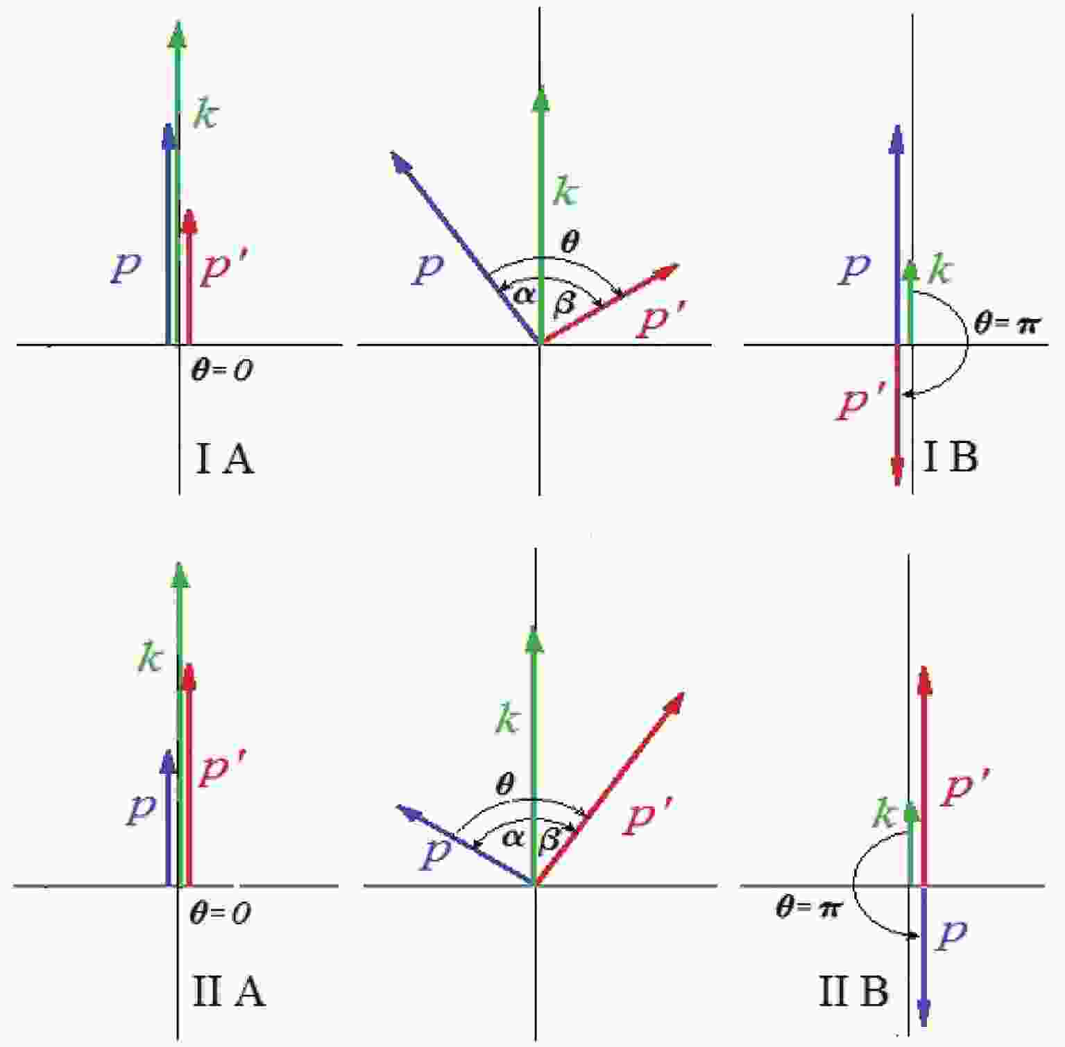
$ \{e\} = \{\vec{e}_1,\vec{e}_2,\vec{e}_3\} $ in the momentum space where$ \vec{k} = \vec{p}+\vec{p}' = k(\theta) \vec{e}_3 $ and the vectors$ \vec{p} $ and$ \vec{p}' $ are in the plane$ \{\vec{e}_1,\vec{e}_3\} $ , as shown in Fig. 1, and have spherical coordinates$ \vec{p} = (p,\alpha,0) $ and$ {\vec{p}\,}' = (p',\beta,\pi) $ such that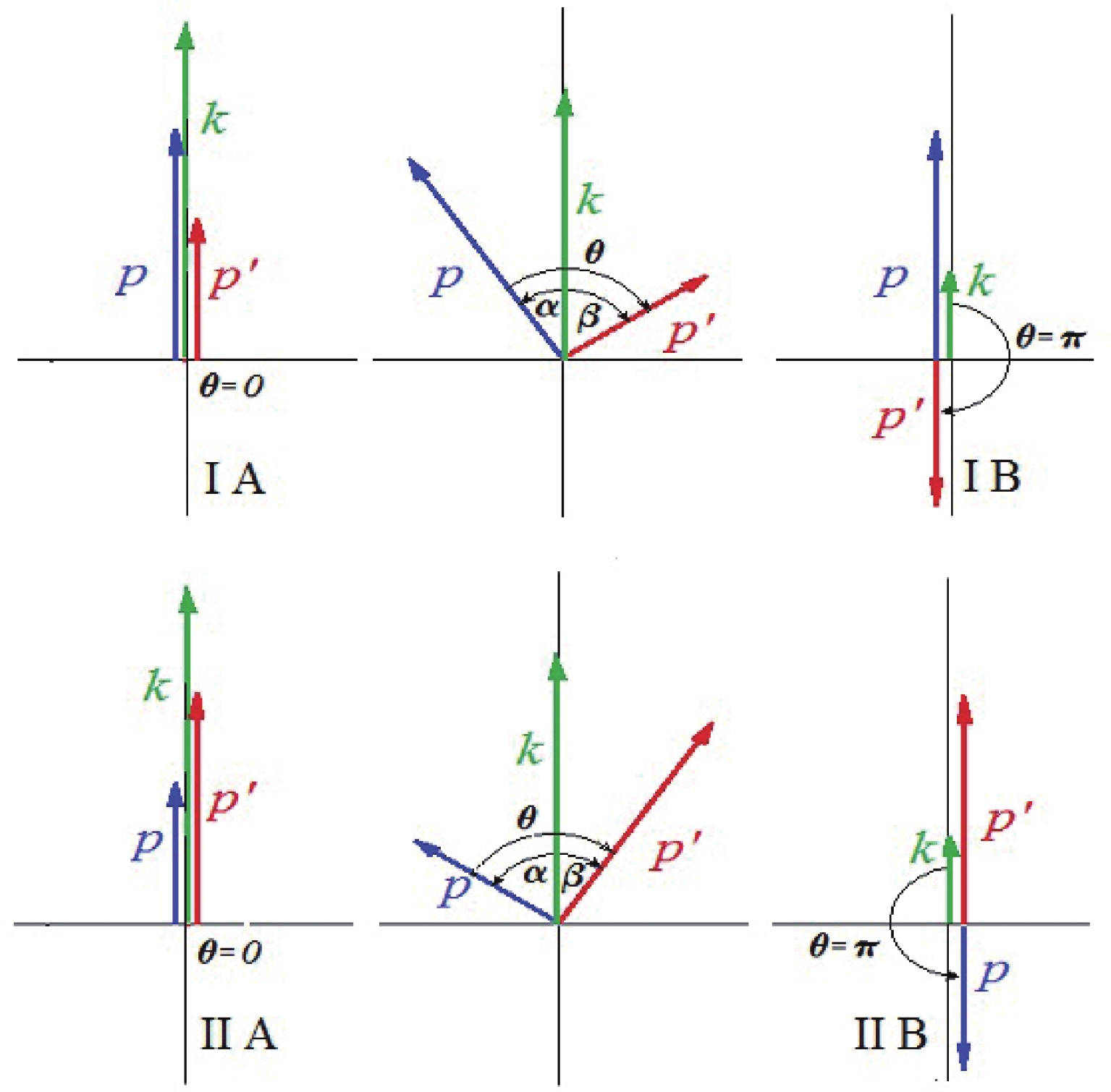
Figure 1. (color online) Pair production in the frame
$\{e\}$ . (I) for$p>p'$ : (I A)$\theta = 0$ $\to$ $k = p+p'$ ,$\sigma' = \sigma$ and$\lambda = 2\sigma$ , (I B)$\theta = \pi$ $\to$ $k = p'-p$ ,$\sigma' = -\sigma$ and$\lambda = 2\sigma$ ; and (II) for$p<p'$ : (II A)$\theta = 0$ $\to$ $k = p+p'$ ,$\sigma' = \sigma$ and$\lambda = 2\sigma$ , (II B)$\theta = \pi$ $\to$ $k = p'-p$ and$\sigma' = -\sigma$ and$\lambda = -2\sigma$ .$ \theta = \alpha+\beta\,, $

(57) $ p\sin\alpha = p'\sin\beta\,. $

(58) In this geometry the polarization vectors take the simple form
$ \vec{\varepsilon}_{\pm 1}(\vec{k}) = \frac{1}{\sqrt{2}}(\pm \vec{e}_1-i\vec{e}_2) $ that allows to derive the polarization matrices$ {\hat \Pi ^{\lambda = 1}} = \sqrt 2 {\mkern 1mu} \left( {\begin{array}{*{20}{c}} {\cos \dfrac{\alpha }{2}\cos \dfrac{\beta }{2}}&{\cos \dfrac{\alpha }{2}\sin \dfrac{\beta }{2}}\\ {\sin \dfrac{\alpha }{2}\cos \dfrac{\beta }{2}}&{\sin \dfrac{\alpha }{2}\sin \dfrac{\beta }{2}} \end{array}} \right){\mkern 1mu} , $

(59) $ {\hat \Pi ^{\lambda = - 1}} = \sqrt 2 {\mkern 1mu} \left( {\begin{array}{*{20}{c}} {\sin \dfrac{\alpha }{2}\sin \dfrac{\beta }{2}}&{\sin \dfrac{\alpha }{2}\cos \dfrac{\beta }{2}}\\ {\cos \dfrac{\alpha }{2}\sin \dfrac{\beta }{2}}&{\cos \dfrac{\alpha }{2}\cos \dfrac{\beta }{2}} \end{array}} \right){\mkern 1mu} , $

(60) where the matrix elements
$ \left|{\hat \Pi}^{\lambda}_{\sigma,\sigma'}\right| $ are the absolute values of the polarization terms in the frame$ \{e\} $ . We can now choose the free parameters$ p,\,p' $ and θ , since the angles we need for calculating the polarization matrix can be deduced as$ \alpha = {\rm arctan}\left(\frac{p'\sin \theta}{p+p'\cos\theta}\right)\,, $

(61) $ \beta = \theta-{\rm arctan}\left(\frac{p'\sin \theta}{p+p'\cos\theta}\right)\,, $

(62) for
$ p>p' $ , as obtained from Eqs. (57) and (58). For$ p<p' $ , we get similar relations by changing$ \alpha \leftrightarrow \beta $ and$ p \leftrightarrow p' $ , while for$ p = p' $ , we have$ \alpha = \beta = \frac{\theta}{2} $ . Using Eqs. (38) and (39), we obtain the final result for the probability per unit volume and unit time in the frame$ \{e\} $ ,$ \begin{split} {\cal P}^{\lambda}_{\sigma,\sigma'}(p,p',\theta) = & \frac{e_0^2}{(2\pi)^{10}}\,\frac{m\omega}{k(\theta)}\, {e}^{\frac{\pi k(\theta)}{2\omega}}\\ & \times \hat\Pi_{\sigma,\sigma'}^2\,\Delta(p,{\rm sign}(\sigma\sigma')p',k(\theta))\,, \end{split} $

(63) which depends only on the free parameters
$ (p,p',\theta) $ in the polarization term and the function$ \Delta(p,p',k) $ defined by Eq. (42).A similar result can be obtained for the process of lepton creation from vacuum,
$ {\rm vac}\to \gamma + e^- + e^+ $ , with similar parameters, whose rates or probabilities comply with the general rule$ \frac{{\cal P}_{{\rm vac} \to\gamma + e^- + e^+}(p,p',\theta)}{{\cal P}_{\gamma \to e^- + e^+}(p,p',\theta)}\simeq {e}^{-\frac{\pi k(\theta)}{\omega}}\,. $

(64) Thus, only the processes of pair creation from photons and lepton creation from vacuum remain, as well as the combined leptonic creation
$ {\rm vac}\to \gamma +e^- + e^+ \to (e^-+e^+)+$ $e^- +e^+ $ , since the transitions between charged states are forbidden. Note that the inverse processes of pair annihilation,$ e^-+e^+\to \gamma $ and lepton annihilation to vacuum,$ \gamma+e^-+e^+\to {\rm vac} $ , cannot occur since it is not probable that two or three particles meet spontaneously. Thus, we get a simple mechanism for creation of electron-positron pairs from vacuum that could be considered in a cosmological scenario.Finally, we observe that the probabilities and rates calculated here are increasing linearly with the parameter ω , which is just the expansion speed of M. This behavior is different from de Sitter case where these quantities depend on de Sitter-Hubble constant [29].
-
The closed expression (63) allows to study the dependence of the probability on the kinematic parameters and polarizations. We observe that we cannot speak here of polarization conservation since we work in the momentum-helicity basis. Nevertheless, there are some particular situations where the momenta have the same direction and, consequently, the polarizations must be conserved as the spin projections are in the same direction. These situations are obtained either for
$ \theta = 0 $ , as in the panels I A and II A of Fig. 1, where$ \alpha = \beta = 0 \to p' = p+k\,, \quad \lambda = \sigma+\sigma'\,, $

(65) or for
$ \theta = \pi $ , as in the panels II A and II B. In the case I B, we set$ p>p' $ and consequently$ \alpha = 0\,,\beta = \pi \to k = p-p'\,,\quad \lambda = \sigma-\sigma'\,, $

(66) while in the case II B, the situation is reversed such that
$ p<p' $ and$ \alpha = \pi\,,\beta = 0 \to k = p'-p\,, \quad \lambda = \sigma'-\sigma\,. $

(67) Note that when
$ p = p' $ , only the parallel case (I A = II A) remains, since the anti-parallel momenta of equal magnitude lead to$ k = 0 $ for which the photon of the in state disappears.We expect to observe the above selection rules in the plot of the probability Eq. (63) versus θ for fixed values of momenta p and
$ p' $ . An unpleasant surprise is that we find a wrong behavior for the angles$ \theta = 0 $ and$ \theta = \pi $ , for which the selection rules require the probability to vanish if the polarizations are not conserved. This occurs because the function$ \Delta(p,p',k(\theta)) $ becomes singular for$ k\pm(p-p') = 0 $ , as shown in Fig. 2.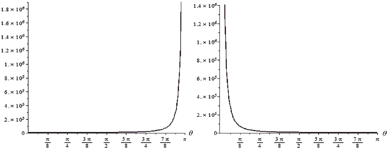
Figure 2. The singular behavior of the functions
$\Delta(p,p',k(\theta))$ (left panel) and$\Delta(p,-p',k(\theta))$ (right panel) for$p = 0.01\,\omega$ and$p' = 0.03\,\omega$ .Thus, we meet again with the difficulties of the perturbation procedures which lead to singularities or violation of conservation laws in some particular direction. In order to extract the physical information we need to remove these singularities by resorting to the method of Yennie et al. [41] of constructing reduced amplitudes by multiplying the obtained amplitudes by suitable trigonometric functions. Thus, for example, the singularity at
$ \theta = 0 $ of the scattering amplitude of various scattering processes can be removed by multiplying the amplitude with$ (1-\cos\theta)^n $ , where n is the reduction order. In our case, a reduction of the first order with$ n = 1 $ is sufficient for eliminating the singularities at$ \theta = 0 $ and$ \theta = \pi $ , and we define the reduced probabilities as$ {\rm Red}\, {\cal P}^{\lambda = \pm 2\sigma}_{\sigma,\sigma}(p,p',\theta) = {\cal P}^{\lambda = \pm 2\sigma}_{\sigma,\sigma}(p,p',\theta) \cos^4\frac{\theta}{2}\,, $

(68) $ {\rm Red}\, {\cal P}^{\lambda = \pm 2\sigma}_{\sigma,-\sigma}(p,p',\theta) = {\cal P}^{\lambda = \pm 2\sigma}_{\sigma,-\sigma}(p,p',\theta) \sin^4\frac{\theta}{2}\,. $

(69) We can now verify that these probabilities match perfectly the selection rules (65)-(67) by plotting them in the whole domain
$ \theta\in [0,\pi] $ , as shown in Figs. 3 and 4. Moreover, we observe that the reduction procedure does not affect the physical content since for the angles$ \theta = 0 $ and$ \theta = \pi $ , for which the function$ \Delta $ is regular, we have$ {\rm Red}\, {\cal P}^{\lambda}_{\sigma,\sigma'} = {\cal P}^{\lambda}_{\sigma,\sigma'} $ , as can be seen in Fig. 3. Thus, we conclude that the reduction procedure is appropriate and allows to understand the physical behavior of the analyzed process.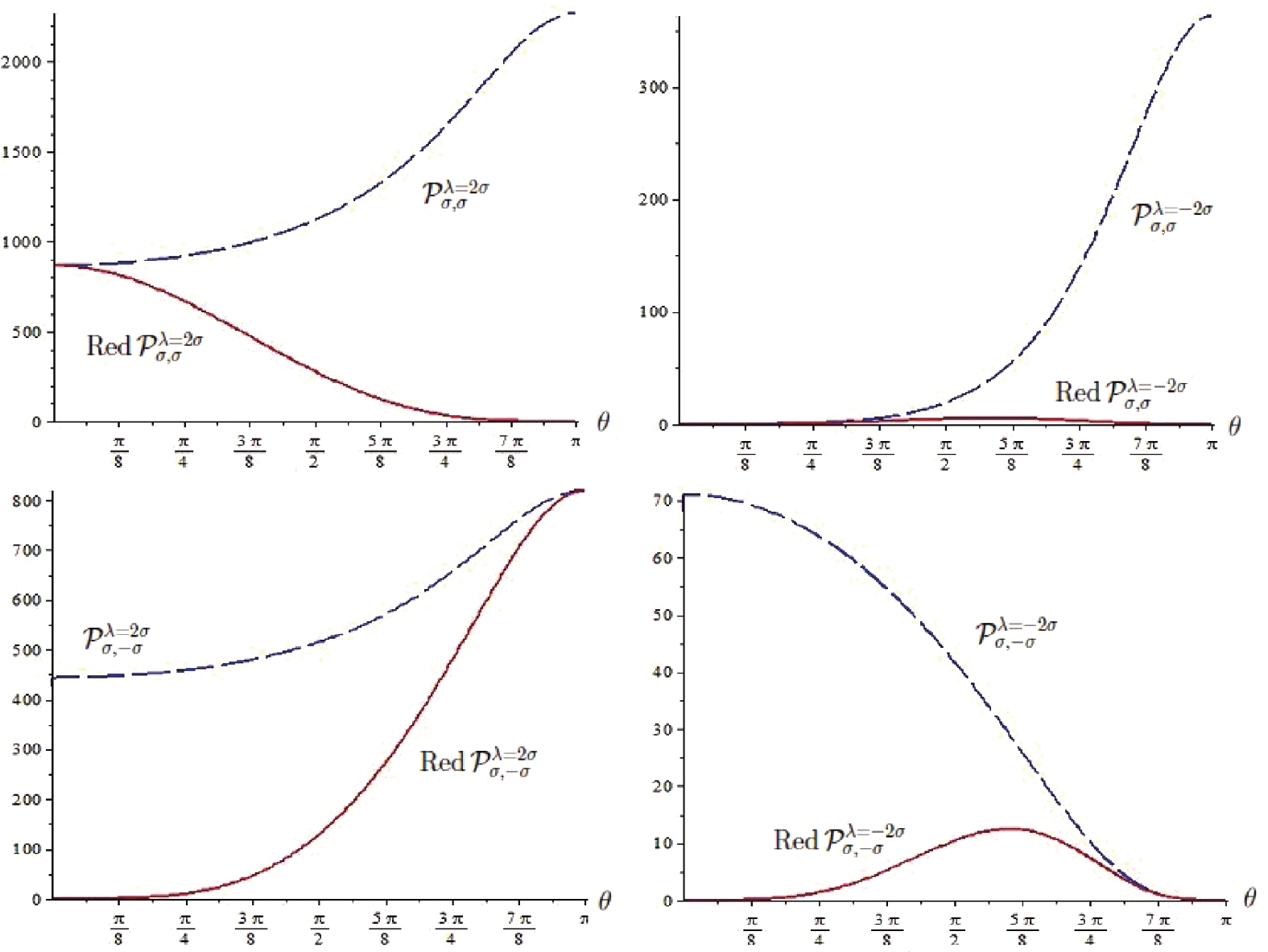
Figure 3. (color online) Results of the reduction procedure: the original (dashed lines) and reduced (solid lines) probabilities versus θ for different polarizations and
$ p = 0.05\, \omega$ and$ p' = 0.02\,\omega$ .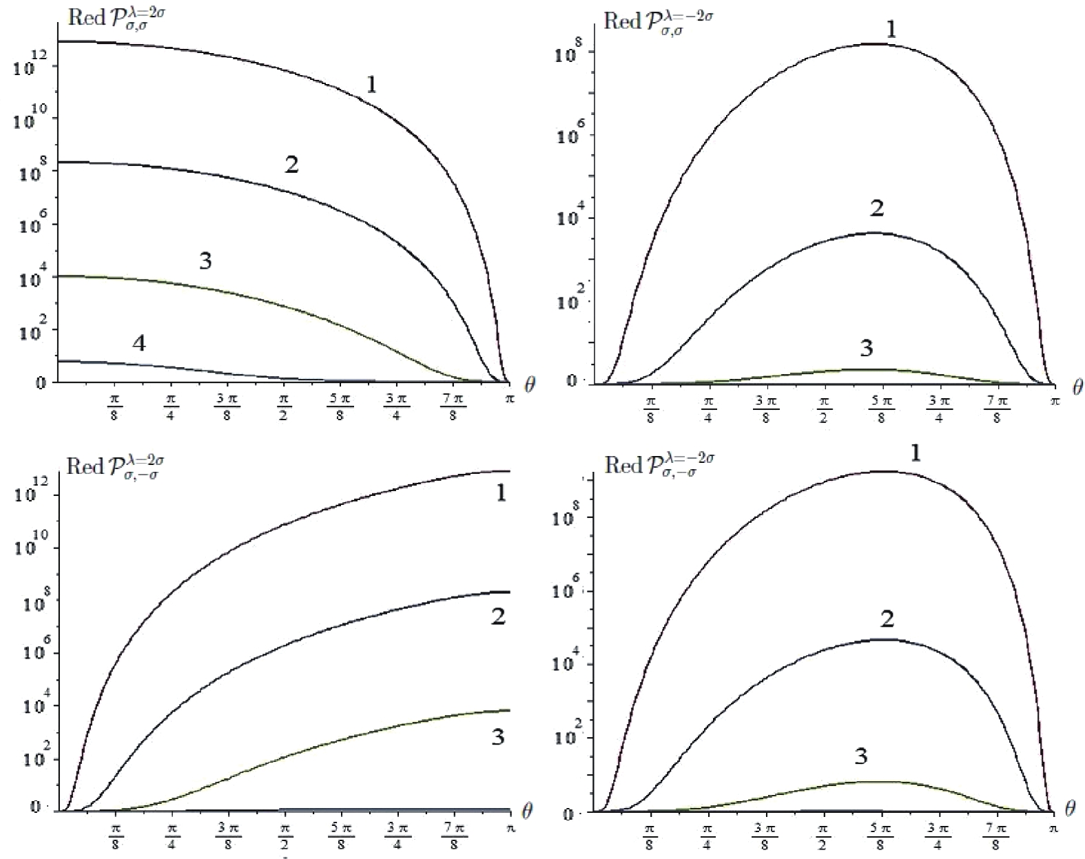
Figure 4. The reduced probabilities versus θ for different polarizations and momenta: (1)
$p = 0.002\, \omega$ and$p' = 0.001\,\omega$ ; (2)$p = 0.02\, \omega$ and$p' = 0.01\,\omega$ ; (3)$p = 0.2\, \omega$ and$p' = 0.1\,\omega$ ; and (4)$p = 2\, \omega$ and$p' = \omega .$ On the other hand, we must say that there is a problem in the divergence at
$ p\sim p' = 0 $ . Indeed, as can be seen in Fig. 4, the reduced probabilities increase when the momenta p and$ p' $ decrease, such that for vanishing momenta the probabilities diverge,$ \lim\limits_{\substack{p\to 0\\p'\to 0}} {\cal P}^{\lambda}_{\sigma,\sigma'} = \lim\limits_{\substack{p\to 0\\p'\to 0}}{\rm Red}\,{\cal P}^{\lambda}_{\sigma,\sigma'} = \infty\,. $

(70) This unwanted effect is somewhat analogous to the infrared catastrophe of the usual QED and could be of interest in an attempt to find infrared regulators or in the vertex renormalization.
-
We studied in this work the quantum fields in the spatially flat FLRW space-time with a Milne-type scale factor (denoted by M). The first impression was that this manifold, which arises from a time singularity, might produce new spectacular physical effects, but our calculations show that, at least from the point of view of quantum theory, this space-time behaves as usual, producing similar effects as de Sitter expanding universe [29]. The only notable new feature is that the first order transitions between charged states are forbidden, but we cannot say if this is specific to this geometry as we do not have other examples.
From the technical point of view, the M and de Sitter space-times have opposite properties, as can be seen from the next self-explanatory table,
$ \begin{array}{*{20}{c}} {}&M&{{\rm{de}}\;{\rm{Sitter}}}\\ t&{0 < t = \dfrac{1}{\omega }{e^{\omega {t_c}}} < \infty }&{ - \infty < t < \infty }\\ {{t_c}}&{ - \infty < {t_c} < \infty }&{ - \infty < {t_c} = - \frac{1}{\omega }{e^{ - \omega t}} < - \dfrac{1}{\omega }\;}\\ {a(t)}&{\omega t}&{{e^{\omega t}}}\\ {a({t_c})}&{{e^{\omega {t_c}}}}&{ - \frac{1}{{\omega {t_c}}}}\\ {u_p^ \pm }&{{K_{\frac{1}{2} \mp i{\kern 1pt} \frac{{2\sigma p}}{\omega }}}(imt)}&{{K_{\frac{1}{2} \mp i\frac{m}{\omega }}}(ip{t_c})} \end{array} $

where we used Eq. (19), and denoted by ω the free parameter in M and the Hubble constant in de Sitter expansion [47]. Thus, we have at least two related examples which help to better understand the perturbative QFT in curved backgrounds, where we have an opportunity for analyzing first order processes which are forbidden in the Minkowski space-time.
Finally, we note that the LSZ formalism applied here is used more or less explicitly for calculating various quantities of interest in cosmology, such as the expectation values, loop corrections and equal-time correlations. Our results show that this formalism is working correctly even in evolving space-times, and gives transition rates of new quantum effects that could be observed in future astrophysical experiments.
-
The Pauli spinors in the momentum-helicity basis,
$ \xi_{\sigma}(\vec{p}) $ , of helicity$ \sigma = \pm\frac{1}{2} $ , satisfy the eigenvalue problem$ (\vec{p}\cdot \vec{S})\,\xi_{\sigma}(\vec{p}) = \sigma\, p\, \xi_{\sigma}(\vec{p}) $ , where$ S_i = \frac{1}{2}\sigma_i $ are the spin operators expressed in terms of Pauli matrices. They have the form$ \tag{A1} \xi_{\frac{1}{2}}(\vec{p}) = \sqrt{\frac{p+p^3}{2p}}\left( \begin{array}{l} \;\;\;1\\ \frac{p^1+i p^2}{p+p^3} \end{array}\right)\,, $

(A1) $ \tag{A2} \xi_{-\frac{1}{2}}(\vec{p}) = \sqrt{\frac{p+p^3}{2p}}\left( \begin{array}{l} \frac{-p^1+i p^2}{p+p^3}\\ \;\;\;\;\;1 \end{array}\right)\,. $

(A2) The antiparticle spinors are usually defined as
$ \eta_{\sigma}(\vec{p}) = i\sigma_2 \xi_{\sigma}(\vec{p})^* $ [40, 45] in order to satisfy$ (\vec{p}\cdot \vec{S})\,\eta_{\sigma}(\vec{p}) = -\sigma\, p\, \eta_{\sigma}(\vec{p}) $ .The polarization of the free Maxwell field is given by the polarization vectors
$ {\vec\varepsilon}_{\lambda}({\vec k}) $ which have complex components. Here, we consider only the circular polarization [40] with$ \vec{\varepsilon}_{\pm 1}(\vec{k}) = \frac{1}{\sqrt{2}}(\pm \vec{e}_1+i\vec{e}_2) $ , in a three-dimensional orthogonal local frame$ \{\vec{e}_i\} $ with$ \vec{k} = k\vec{e}_3 $ . -
Using the general properties of the modified Bessel functions
$ I_{\nu}(z) $ and$ K_{\nu}(z) = K_{-\nu}(z) $ [50], we deduce that$ K_{\nu_{\pm}}(z) $ with$ \nu_{\pm} = \frac{1}{2}\pm i \mu $ are related as$\tag{B1} H^{(1,2)}_{\nu}(z) = \mp\frac{2i}{\pi}{\rm e}^{\mp \frac{\rm i}{2}\pi\nu}K_{\nu}(\mp iz)\,, \quad z\in {\mathbb R}\,. $

(B1) The functions used here,
$ K_{\nu_{\pm}}(z) $ with$ \nu_{\pm} = \frac{1}{2}\pm i \mu $ ($ \mu \in {\mathbb R} $ ), are related as$ \tag{B2} [K_{\nu_{\pm}}(z)]^{*} = K_{\nu_{\mp}}(z^*)\,,\quad \forall z \in{\mathbb C}\,, $

(B2) satisfy the equations
$\tag{B3} \left(\frac{\rm d}{\rm dz}+\frac{\nu_{\pm}}{z}\right)K_{\nu_{\pm}}(z) = -K_{\nu_{\mp}}(z)\,, $

(B3) and the identities
$ \tag{B4} K_{\nu_{\pm}}(iz)K_{\nu_{\mp}}(-iz)+ K_{\nu_{\pm}}(-iz)K_{\nu_{\mp}}(iz) = \frac{\pi}{ |z|}\,, $

(B4) which guarantee the correct orthonormalization properties of the fundamental spinors. For
$ z\to \infty $ , these functions behave as [50]$\tag{B5} I_{\nu}(z) \to \sqrt{\frac{\pi}{2z}}e^{z}\,, \quad K_{\nu}(z) \to K_{\frac{1}{2}}(z) = \sqrt{\frac{\pi}{2z}}e^{-z}\,, $

(B5) regardless of the index ν.
Moreover, here we use the integral (6.576-4) of Ref. [51] with
$ b = \pm a $ ,$ \tag{B6} \begin{split} \int_{0}^{\infty}{\rm d}x\,x^{-\lambda}K_{\mu}(ax) K_{\nu}(\pm ax) =& \frac{(\pm)^{\nu}\,2^{-2-\lambda} a^{\lambda-1}}{\Gamma(1-\lambda)}\\ & \times\Gamma\left(\frac{1-\lambda+\mu+\nu}{2}\right)\Gamma\left(\frac{1-\lambda-\mu+\nu}{2}\right) \\ & \times\Gamma\left(\frac{1-\lambda+\mu-\nu}{2}\right)\Gamma\left(\frac{1-\lambda-\mu-\nu}{2}\right)\,. \end{split} $

(B6)
First order QED processes in a spatially flat FLRW space-time with a Milne-type scale factor
- Received Date: 2019-12-07
- Available Online: 2020-05-01
Abstract: The quantum electrodynamics (QED) in a spatially flat (1+3)-dimensional Friedmann-Lemaître-Robertson-Walker (FLRW) space-time with a Milne-type scale factor is outlined focusing on the amplitudes of the allowed processes in the first order perturbations. The definition of the transition rates is reconsidered such that an appropriate angular behavior of the probability for creation of an electron-positron pair from a photon is obtained, which has a similar rate as the creation of a photon and an electron-positron pair from vacuum. It is shown that these processes are allowed only in the first order perturbations, since the photon emission or absorption by an electron or positron are forbidden.


 DownLoad: