


 Abstract
 HTML
HTML Reference
 Related
 PDF
PDF


-
It is widely believed that our universe started with a hot big bang, which is considered as the beginning of the radiation-dominated era in cosmic history. Numerous properties of the cosmos that we observe today can be understood as consequences of quantum processes, which are typically out of equilibrium in the hot and dense plasma [1, 2] that filled the universe after the big bang. Prior to the radiation dominated era, there was a period of accelerated cosmic expansion known as inflation [3–5]. At the end of inflation, the universe was cold and empty; all energy was stored in the zero mode of the inflaton field. One mechanism for setting up the initial conditions of a "hot big bang" of the radiation-dominated universe is "reheating" [6–8], where the universe is "reheated" from a complete vacuum by energy transfer from the inflaton to other degrees of freedom, e.g., dark matter particles and elementary particles that made up the standard model (SM) of particle physics. The study of the quantum dissipative effects in the early universe, therefore, has profound implications on the studies of matter production and thus on the thermal history of our universe.
The thermal history of the early universe is an important theoretical basis to determine the abundance of thermal relics. It thus plays an important role in distinguishing or excluding cosmological models. Studies of the particle dynamics in the early universe uncover crucial details within and beyond the SM. We are interested in the thermal production of particles from plasma [9, 10], dissipation effects of fields in medium [11, 12], cosmological freeze-out processes [13, 14], and their imprints on early universe physics.
As mentioned above, matter production occurs through the relaxation of inflaton into scalar, gauge, and fermionic quantum fields in a large thermal bath [9, 15–17]. Inflaton, in the SM of cosmology, is a scalar and responsible for an epoch of exponential expansion to produce a flat, homogeneous, and isotropic universe free of topologically stable relics, such as monopoles and cosmic strings. Therefore, scalar fields, despite their simplicity, play important roles within or beyond the SMs of particle physics and modern cosmology. The existence of scalar fields in the SM of Particle physics has been firmly established by high precision experiments conducted at the large hadron collider (LHC) in 2012, where the Higgs boson [18, 19] plays a pivotal role of providing mass to elementary particles in the SM. Furthermore, scalar fields can be candidates for dark energy [20–22] or dark matter [23–25]. Scalar fields also play important roles in the bounce universe, which is an alternative approach to address how our current universe came about. In this model, a contraction phase exists prior to the "birth" of our presently observed universe, and further detail is provided in recent reviews in Refs. [26, 27] . Our study focuses on the scalar field dynamics in hot medium: it thus founds the basis to follow up on the particle productions in these bounce models [28–34], where the Hubble parameter can be set to positive or negative values, and the bounce process is driven by two or more scalar fields.
This study builds on an earlier study of the finite-temperature effects in a thermal bath, carried out by Y. K. E. Cheung, M. Drewes, J. U Kang, and J. C. Kim , to further establish the rigorous theoretical framework to precisely study the evolution and interactions of elementary fields in the inflationary cosmology background or in a bounce universe. In Ref. [35], the authors made progress towards a quantitative understanding of the non-equilibrium dynamics of scalar fields in the non-trivial background of the early universe with a high temperature, large energy density, and a rapid cosmic expansion. They calculated the effective action and quantum dissipative effects of a cosmological scalar field in this background. The analytic expressions for the effective potential and damping coefficient are presented using a simple scalar model with quartic interaction. In this paper, we extend their efforts on building this theoretical framework by incorporating a non-zero Hubble parameter in the analysis and obtain a temperature-dependent expression of the damping coefficient to the first order in H. In this manner, one can properly address the questions of how the hot primordial plasma may have been created after inflation [36] and whether there are observable features in the reheating process [37, 38].
Our study of the non-equilibrium process in an early universe starts from the action of scalar fields ϕ and χ. The non-equilibrium process is non-Markovian. That is, the evolution of the fields in late times depends on all previous states, and the non-Markovian effects are contained in a "memory integral" in the Kadanoff-Baym equations. We shall use the closed-time-path (CTP) formalism [39, 40], i.e., the so-called "in-in formalism". The "in-in formalism" is made to deal with such finite temperature problems in out-of-thermal-equilibrium processes. The non-equilibrium nature renders the usual "in-out formalism" ineffective.
Unlike the usual zero-temperature quantum field theory, this study considers both the thermal and quantum corrections. To be more specific, we first derive the equation of motion, up to the first order in H, from the effective action of ϕ. The effective potential and the dissipation coefficient (characterizing the dissipation of the energy from ϕ to the plasma) rely on the self-energy and the corrections to the quartic coupling constant. The calculations of these quantities using Feynman diagrams make up a major part of work reported in this article. If we set H to 0, our results match up with those obtained in Ref. , using a Minkowski-space propagator in loops. Furthermore, we observe non-trivial features that are not revealed in flat spacetime.
Exposing scalar fields to a high temperature and a rapid cosmic expansion is an important setup for understanding the non-equilibrium dynamics of scalar fields in cosmology. Under the condition of cosmic expansion at high temperatures, the matter production process is out of equilibrium. If there is an effective potential that is not steep, the matter fields take a long time to reach equilibrium. Our focus is the back reaction [41, 42] on the primary particles from their decay products. Based on the previous work done using Minkowski-space propagators in loop diagrams, we further their studies of scalar field dynamics in the early universe evolution by incorporating the effect of cosmic expansion. There are infinitely many back reactions, and thus it is important to generalize the leading-order re-summation results to higher orders.
Although elementary particles in our universe comprise fermions and gauge bosons, we still expect our toy model with two scalar fields to serve as a good playground for studying early universe physics. The earliest decay process involves only scalars, because the creation of fermions can be assumed to occur in the subsequent decay chain or inelastic scatterings, as the transition to bosonic states is usually Bose-enhanced [8]. When the background temperature is higher than the oscillation frequency, the dissipation rate arising from the interactions with fermions is suppressed due to Pauli blocking, whereas it is enhanced for interactions with bosons due to the induced effect. In a future study, we will consider the direct coupling of scalars to fermions and gauge bosons.
The study of thermal dynamics of fields in curved spacetime is technically very difficult. For the first order in the Hubble parameter, the calculation of scalar dynamics might shed light on the effects of the expansion of the universe on its history. More specifically, this is a step further into the investigation of the microscopical process that happened during reheating, preheating, and warm inflation, where the dissipative process including effective friction and potentials should be described.
The results presented in this study represent another step in a systematic study of scalar dynamics in the early universe, as initiated in . The analytic expressions we find are derived more systematically and consistently than any comparable results in the literature that we are aware of. The current paper adds to this program by including the expansion of the background spacetime to the analytic estimates for effective potentials and dissipation coefficients. Moreover, in the course of the derivation, we find analytic estimates for various integrals in finite-temperature field theory that will be very useful for calculations in more realistic models, in spite of the limitations of the toy model we employed to set up our calculations. This paper is organized as follows: in Section 2, we explain our working assumptions. We sketch the prerequisites for field theory calculations at finite temperature to establish notations, which is followed by the derivation of the EoM in Section 3. We demonstrate the calculations of self-energy and obtain the correction to the quartic coupling constant in Section 4. Section 5 briefly summarizes the main results obtained in this paper and concludes with a short discussion. The detailed calculations of the Feynman diagrams and the relevant formulae needed in the calculations are presented in the appendices.
-
We study a scalar field, denoted by ϕ, in a de Sitter space with the Hubble parameter H assumed to be nonzero. The scalar field ϕ interacts with other significantly lighter scalar fields, collectively denoted by χ, which play the role of the hot cosmic bath in our model. (The typical picture for this setting is the decay of inflaton (ϕ) at the end of inflation to the array of elementary particles of the Standard Model, a process called "reheating".)
Let ϕ be decomposed into its thermal average, φ, and its fluctuations, denoted by η:
$ \phi = \varphi+\eta. $

The fields η and χ are initially assumed to be in thermal equilibrium. We further assume that the interactions between φ and other degrees of freedom are sufficiently weak to allow for the application of perturbation theory and the neglecting of back reaction of φ on the η and χ fields. The approximately adiabatic evolution of φ can be assumed. In this way, η and χ can assume thermal equilibrium in the evolution of φ.
To expand the equation of motion to the first order in H and simplify the calculations, we further assume that
$ H < M_{\eta}, M_{\chi} \ll T $ , where$ M_{\eta} $ and$ M_{\chi} $ are, respectively, the effective masses of η and χ, and the temperature T is inversely proportional to the scale factor.The field ϕ is to decay to χ, and hence
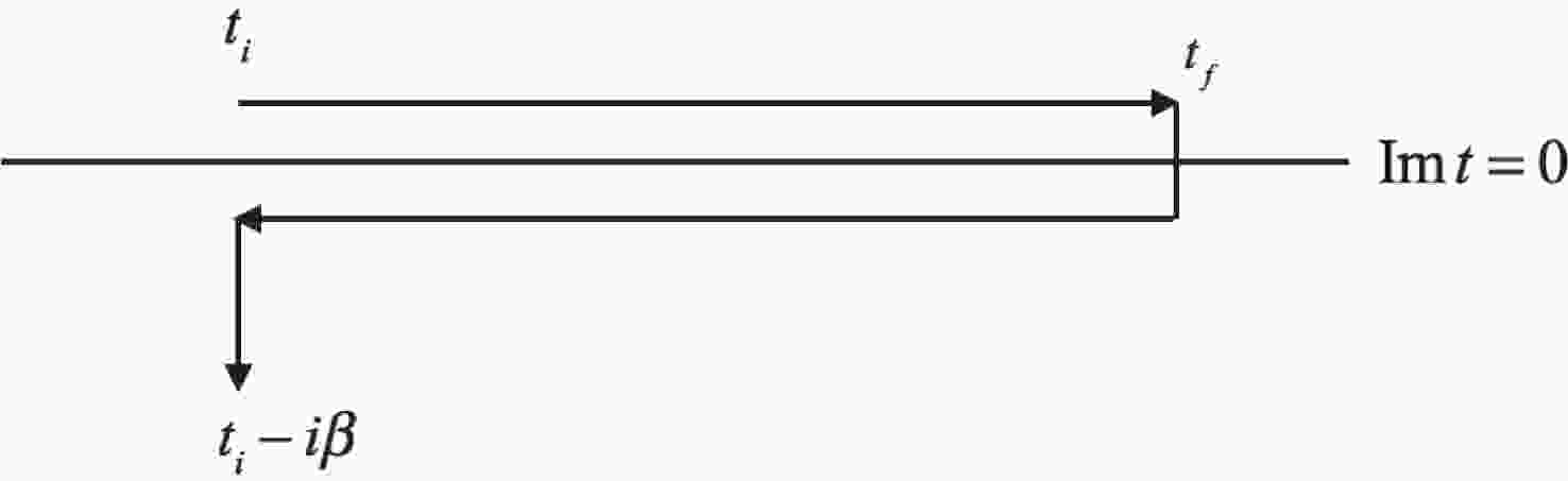
$ M_{\eta} \geq 2M_{\chi} $ . However, in the ensuing calculations, we cannot obtain analytical results unless$ M_{\eta}\gg M_{\chi} $ . We will thus take$ M_{\eta}\gg M_{\chi} $ as an assumption instead①. For the same purpose, we assume that$ \lambda, \lambda', h \ll M_{\chi} \gamma $ , where$ \lambda, \lambda', h $ are coupling constants and γ is essentially the inverse temperature that will be introduced soon in the following content. There is a sufficiently long period of time in our universe, in which these conditions are satisfied, and matter creation due to the decay of inflaton, ϕ, to other fields$ \chi_{i} $ can be studied in this systematic approach.Methodology: We use the closed-time-path formalism to perform the calculations. The readers are referred to [43–45] for systematic introductions to field theory at finite temperature. The time ordering and integration path C in the complex time plane starts from
$ t_i $ on the real axis and runs to real$ t_f $ , then back to$ t_i $ and ends at$ t_i-i\beta $ , as depicted in Fig. 1.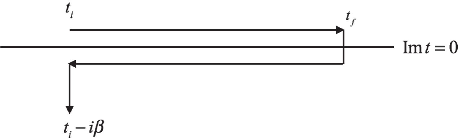
Figure 1. Path of integration in complex-time plane.
We take
$ t_i \to -\infty $ and$ t_f\to\infty $ and denote the upper section of C, which runs forward in time by$ C_1 $ and the lower section, which runs backward in time by$ C_2 $ . A general scalar field$ \xi(x) $ that lies on$ C_1/C_2 $ is labelled as$ \xi_1(x) $ /$ \xi_2(x) $ .To obtain the dynamical information of such a scalar field ξ, we need to know the two-point correlation functions that are defined as follows,
$ \begin{split} \Delta_{ab}(x,y) =& \langle T_C\xi_a(x)\xi_b(y) \rangle \quad (a,b = 1,2),\\ \Delta^>(x,y) =& \langle\xi(x)\xi(y)\rangle,\quad \Delta^<(x,y) = \langle\xi(y)\xi(x)\rangle,\\ \Delta^-(x,y) =& i\left[\Delta^>(x,y)-\Delta^<(x,y)\right],\\ \Delta^+(x,y) =& \frac{1}{2}\left[\Delta^>(x,y)+\Delta^<(x,y)\right], \end{split} $

(1) where
$ T_C $ indicates time ordering along the path C in Fig. 1. For a real scalar field ξ, we see that$\Delta^{>}(x,y) = $ $ {(\Delta^<(x,y))}^{*} $ and that$ \begin{split} \Delta_{11}(x,y) =& \theta(x^0-y^0)\Delta^{>}(x,y)+\theta(y^0-x^0)\Delta^{<}(x,y),\\ \Delta_{22}(x,y) =& \theta(x^0-y^0)\Delta^{<}(x,y)+\theta(y^0-x^0)\Delta^{>}(x,y),\\ \Delta_{12}(x,y) =& \Delta^{<}(x,y),\\ \Delta_{21}(x,y) =& \Delta^{>}(x,y). \end{split} $

(2) The one-loop propagators of a scalar field ξ with effective mass
$ M_\xi $ in a de-Sitter space,$ g_{\mu\nu} = {\rm{diag}}(1,-a(t)^2,-a(t)^2,-a(t)^2), $

(3) where
$ a(t) = {\rm e}^{Ht} $ , were obtained by solving the Kadanoff-Baym equations [43]. The result in Ref. [43] is expressed in terms of conformal time, with a time-dependent mass$ m(t) $ . To obtain the corresponding result in terms of cosmic time, we first carry out the usual replacement:$ t\to -\frac{1}{Ha(t)}\; . $

(4) The following two replacements can be inferred by comparing the free spectral function in de Sitter spacetime (whose detailed calculation is presented in Appendix A) with the corresponding flat-spacetime propagator [43]:
$ \xi(x)\to \xi(x)/a(t),\quad m(t)^2\to \left(M_\xi^2-2H^2\right)a(t)^2\; . $

(5) We thus start our calculations with the following propagators in de Sitter spacetime:
$ \left\{ \begin{split} &\Delta^{-}({{p}},t_1,t_2) = \dfrac{ \sin\left(\displaystyle\int_{t_2}^{t_1}{\rm d}t'\Omega_\xi(t')\right)\exp\left(-\dfrac{1}{2}\left|\displaystyle\int_{t_2}^{t_1}{\rm d}t' \Gamma_\xi(t')\right|\right)}{a(t_1)^{3/2}a(t_2)^{3/2}\sqrt{\Omega_\xi(t_1)\Omega_\xi(t_2)}}\\ & \Delta^{+}({{p}},t_1,t_2) = \left[1+2f(t_B)\right] \cdot \dfrac{ \cos\left(\displaystyle\int_{t_2}^{t_1}{\rm d}t'\Omega_\xi(t')\right)\exp\left(-\dfrac{1}{2}\left|\displaystyle\int_{t_2}^{t_1}{\rm d}t' \Gamma_\xi(t')\right|\right)}{2a(t_1)^{3/2}a(t_2)^{3/2}\sqrt{\Omega_\xi(t_1)\Omega_\xi(t_2)}}\; , \end{split} \right. $

(6) where
$ \Gamma_\xi $ is the decay rate of ξ,$ \Omega_\xi $ is given by$ \Omega_\xi(t) = \sqrt{{{p}}^2/a(t)^2+M_\xi^2-2H^2}\; , $

(7) with
$ t_B = \min(t_1,t_2) $ , and$ f(t) $ satisfies a Markovian equation [43].If we assume that a scalar field ξ is in (approximate) thermal equilibrium as the universe expands, and that it can be characterized by an effective temperature
$ 1/\beta(t) $ , which depends on time, then by imposing the Kubo-Martin-Schwinger (KMS) relations, the propagators become$ \left\{ \begin{split}\Delta^{-}({{p}},t_1,t_2) =& \dfrac{ \sin\left(\displaystyle\int_{t_2}^{t_1}{\rm d}t'\Omega_\xi(t')\right)\exp\left(-\dfrac{1}{2}\left|\displaystyle\int_{t_2}^{t_1}{\rm d}t' \Gamma_\xi(t')\right|\right)}{a(t_1)^{3/2}a(t_2)^{3/2}\sqrt{\Omega_\xi(t_1)\Omega_\xi(t_2)}}\\ \Delta^{+}({{p}},t_1,t_2) = & \dfrac{1}{2a(t_1)^{3/2}a(t_2)^{3/2}\sqrt{\Omega_\xi(t_1)\Omega_\xi(t_2)}}\exp\left(-\frac{1}{2}\left|\int_{t_2}^{t_1}{\rm d}t' \Gamma_\xi(t')\right|\right) \left\{ \exp\left(-{\rm i}\int_{t_2}^{t_1}{\rm d}t'\Omega_\xi(t')\right)\left[\frac{1}{2}+f\left(\Omega_\xi\left(t_B\right)+\frac{{\rm i}\Gamma_\xi\left(t_B\right)}{2}\right)\right]\right.\\ & \left.+\exp\left({\rm i}\int_{t_2}^{t_1}{\rm d}t'\Omega_\xi(t')\right)\left[\frac{1}{2}+f\left(\Omega_\xi\left(t_B\right)-\frac{{\rm i}\Gamma_\xi\left(t_B\right)}{2}\right)\right]\right\}\; , \end{split} \right.$

(8) where f becomes the Bose distribution function:
$ f(x) = \frac{1}{{\rm e}^{\beta(t)x}-1}\; . $

(9) Here, the inverse temperature
$ \beta(t) $ is proportional to the scale factor by our assumptions:$ \beta(t) = (\beta_0/a_0)a(t) $ with$ \beta_0 $ being the inverse temperature when the scale factor is$ a_0 $ . For simplicity, we denote$ \beta_0/a_0 $ by γ in the following calculations:$ \beta(t) = \frac{\beta_0}{a_0}a(t)\equiv\gamma a(t). $

(10) -
As mentioned in the Introduction, our system consists of a scalar field ϕ and the background plasma collectively denoted by χ. We employ the model to study the early universe dynamics: it provides us with clues on how the fields behave in an expanding or contracting universe. In particular, we wish to capture how their behaviour differs as one goes beyond using the Minkowski propagator in computing the quantum and thermal corrections. A general renormalizable action for such a system in a de-Sitter space, whose potential energy is bounded from below, is of the form:
$ \begin{split} S =& -\int {\rm d}^4x\sqrt{-g}\left\{\frac{1}{2}\phi\left[\frac{1}{\sqrt{-g}}\partial_{\mu}\left(\sqrt{-g}g^{\mu\nu}\partial_{\nu}\right)+m_\phi^{2}+Z R\right]\phi\right.\\ & \left.+\frac{1}{2}\chi\left[\frac{1}{\sqrt{-g}}\partial_{\mu}\left(\sqrt{-g}g^{\mu\nu}\partial_{\nu}\right)+m_{\chi}^{2}+Z R\right]\chi\right.\\ & \left.+\frac{\lambda}{4!}\phi^4+\frac{\lambda'}{4!}\chi^4+\frac{h}{4}\phi^2\chi^2\right\}. \\[-15pt]\end{split} $

(11) where
$ R = 6(\ddot{a}/a+\dot{a}^2/a^2) $ is the curvature scalar, and Z is a parameter. The action is furthermore invariant under diffeomorphism and$ \phi(x)\to -\phi(x) $ .The effective action for φ (which can be used to obtain the equation of motion of φ) has the same linear symmetries as the original action [46], it can be written in the form,
$ \begin{split} \Gamma =& -\frac{1}{2}\int_C {\rm d}^4x_1\sqrt{-g}\varphi(x_1)\left[\frac{1}{\sqrt{-g}}\partial_{1\mu}\left(\sqrt{-g}g^{\mu\nu}\partial_{1\nu}\right)+m_\phi^{2}+Z R\right]\varphi(x_1)\\ & -\frac{1}{2}\int_C \sqrt{-g(x_1)}\sqrt{-g(x_2)}{\rm d}^4x_1{\rm d}^4x_2\Pi(x_1,x_2)\varphi(x_1)\varphi(x_2)\\ & -\int_C\sqrt{-g(x_1)}\sqrt{-g(x_2)}{\rm d}^4x_1{\rm d}^4x_2\frac{1}{4!}\left[\lambda\frac{\delta^4(x_1-x_2)}{\sqrt{-g(x_1)}}+\widetilde{\Pi}(x_1,x_2)\right]\varphi(x_1)^2\varphi(x_2)^2,\end{split}$

(12) up to the fourth power of φ. In doing so, we have only considered terms up to one-loop in the quartic part, and the time integration is along the path C, shown in Fig. 1. Π is the self-energy, and
$ \widetilde{\Pi} $ the correction to the quartic coupling constant, the computation of which will be presented in the following section. Similar to the case of propagators, we will denote$ \Pi(x_1,x_2) $ as$ \Pi_{ab}(x_1,x_2) $ when$ x_1^0 $ lies on$ C_a $ and$ x_2^0 $ lies on$ C_b $ ($ a,b = 1\, {\rm{or}}\, 2 $ ). Different from the situation in flat spacetime, here we do not have time translation symmetry:$ \Pi(x_1,x_2),\widetilde{\Pi}(x_1,x_2) $ depend not only on$ t_1-t_2 $ , but on$ t_1+t_2 $ as well.From Eq. (12) we obtain the equation of motion for φ,
$ \begin{split} \frac{\delta\Gamma}{\delta\varphi(x_1)} =& {\rm e}^{3Ht_1}\left(\partial_{0}^{2}+3H\partial_0-{\rm e}^{-2Ht_1}\nabla^2+m_\phi^2+Z R\right)\varphi(x_1)+\int_C {\rm d}x_2 {\rm e}^{3H(t_1+t_2)}\Pi(x_1,x_2)\varphi(x_2)\\ &+\frac{\lambda}{3!}\varphi(x_1)^3{\rm e}^{3Ht_1}+\frac{1}{3!}\varphi(x_1)\int_C {\rm d}x_2{\rm e}^{3H(t_1+t_2)}\widetilde{\Pi}(x_1,x_2)\varphi(x_2)^2\, = \, 0\; . \end{split} $

(13) We restrict ourselves to the case in which the only non-vanishing Fourier mode of
$ \varphi(x) $ is$ \varphi({{q}} = 0) $ , then in (spatial) momentum space, EoM simplifies to$ \begin{split} 0 = & \left(\partial_{0}^{2}+3H\partial_0+m_\phi^2+Z R\right)\varphi(t_1)+\int_C {\rm d}t_2 {\rm e}^{3Ht_2}\Pi(t_1,t_2)\varphi(t_2)\\ &+\frac{\lambda}{3!}\varphi(t_1)^3+\frac{1}{3!}\varphi(t_1)\int_C {\rm d}t_2{\rm e}^{3Ht_2}\widetilde{\Pi}(t_1,t_2)\varphi(t_2)^2. \end{split} $

(14) This non-local equation remains difficult to solve. To make progress, the Hubble parameter H is assumed to be small and the system is in pseudo-equilibrium during the process. This is a valid hypothesis for most of the physical applications we have in mind. In particular, we are interested in the matter productions from vacuum after inflation ends. We can hence simplify the equation by neglecting the curvature scalar term (since
$ R\propto H^2 $ ) and expanding$ {\rm e}^{3Ht_2} \approx1+3Ht_2 $ to the first order in H; while the adiabatic assumption is realized as$ \varphi(t_2)\approx$ $ \varphi(t_1)+\dot{\varphi}(t_1)(t_2-t_1) $ . Altogether,$ \begin{split} &\left(\partial _{0}^{2}+3H\partial _0+m_\phi^2\right)\varphi(t_1)+\int_{-\infty}^{\infty}{\rm d}t_2(1+3Ht_2)\Pi^R(t_1,t_2)\left[\varphi(t_1)+\dot{\varphi}(t_1)(t_2-t_1)\right] \\ & \quad +\frac{\lambda}{3!}\varphi(t_1)^3 +\frac{1}{3!}\varphi(t_1)\int_{-\infty}^{\infty}{\rm d}t_2(1+3Ht_2)\widetilde{\Pi}^R(t_1,t_2)\left[\varphi(t_1)^2+2\varphi(t_1)\dot{\varphi}(t_1)(t_2-t_1)\right] = 0 \; . \end{split} $

(15) Let
$ \Pi^{R}(t_1,t_2) $ denote the retarded self-energy:$ \Pi^{R}(t_1,t_2) = \Pi_{11}(t_1,t_2)+\Pi_{12}(t_1,t_2), $

(16) and likewise,
$ \widetilde{\Pi}^R(t_1,t_2) $ denotes the "retarded" correction to self-coupling,$ \widetilde{\Pi}^R(t_1,t_2) = \widetilde{\Pi}_{11}(t_1,t_2)+\widetilde{\Pi}_{12}(t_1,t_2)\; . $

(17) The Fourier transformations of
$ \Pi^R(t_1,t_2) $ and$ \widetilde{\Pi}^R(t_1,t_2) $ (with respect to$ t = t_1-t_2 $ ) are denoted by$ \kappa(t_1,\omega) $ and$ \widetilde{\kappa}(t_1,\omega) $ :$ \begin{array}{l} \kappa(t_1,\omega)\equiv \displaystyle\int {\rm d}t\,\,\Pi^R(t_1,t_1-t){\rm e}^{{\rm i}\omega t},\\ \widetilde{\kappa}(t_1,\omega)\equiv \displaystyle\int {\rm d}t\,\,\widetilde{\Pi}^R(t_1,t_1-t){\rm e}^{{\rm i}\omega t}\; . \end{array} $

(18) The equation of motion for φ thus takes this form,
$ \ddot{\varphi}(t_1)+\partial_\varphi V(\varphi,t_1)+(3H+\Gamma(\varphi,t_1))\dot{\varphi}(t_1) = 0 $

(19) where the potential
$ V(\varphi,t_1) $ and the dissipation coefficient$ \Gamma(\varphi,t_1) $ are defined as follows,$ \begin{split} \partial_\varphi V(\varphi,t_1)\equiv &\left[m_\phi^2+(1+3Ht_1) {\kappa}(t_1,\omega = 0)-3H\left(-{\rm i} \left.\frac{\partial }{\partial \omega} {\kappa}(t_1,-\omega)\right|_{\omega = 0} \right)\right]\varphi(t_1)\\ & +\frac{1}{6}\left[\lambda+(1+3Ht_1) {\widetilde{\kappa}}(t_1,\omega = 0)-3H\left(-{\rm i}\left.\frac{\partial }{\partial \omega} {\widetilde{\kappa}}(t_1,-\omega)\right|_{\omega = 0}\right)\right]\varphi(t_1)^3,\\ \Gamma(\varphi,t_1)\equiv &-(1+3Ht_1)\left(-{\rm i} \left.\frac{\partial }{\partial \omega} {\kappa}(t_1,-\omega)\right|_{\omega = 0} \right)-3H \left.\frac{\partial^2 }{\partial \omega^2} {\kappa}(t_1,-\omega)\right|_{\omega = 0} \\ & +\frac{1}{3}\left[-(1+3Ht_1)\left(-{\rm i}\left.\frac{\partial }{\partial \omega} {\widetilde{\kappa}}(t_1,-\omega)\right|_{\omega = 0}\right)-3H\left.\frac{\partial^2 }{\partial \omega^2} {\widetilde{\kappa}}(t_1,-\omega)\right|_{\omega = 0}\right]\varphi(t_1)^2. \end{split} $

From this equation of motion, we see that the "potential", which is time-dependent for φ, is determined by
$ {\kappa}(t_1,\omega = 0) $ ,$ {\widetilde{\kappa}}(t_1,\omega = 0) $ ,$ \left.\frac{\partial }{\partial \omega} {\kappa}(t_1,-\omega)\right|_{\omega = 0} $ ,$ \left.\frac{\partial }{\partial \omega} {\widetilde{\kappa}}(t_1,-\omega)\right|_{\omega = 0} ; $ whereas the dissipation coefficient (terms in the second curly bracket) relies on$ \left.\frac{\partial }{\partial \omega} {\kappa}(t_1,-\omega)\right|_{\omega = 0} $ ,$ \left.\frac{\partial }{\partial \omega} {\widetilde{\kappa}}(t_1,-\omega)\right|_{\omega = 0} $ ,$ \left.\frac{\partial^2 }{\partial \omega^2} {\kappa}(t_1,-\omega)\right|_{\omega = 0} $ ,$ \left.\frac{\partial^2 }{\partial \omega^2} {\widetilde{\kappa}}(t_1,-\omega)\right|_{\omega = 0} $ . We will obtain these expressions in the following section. -
In this section, we shall calculate the self-energy and the correction to the self-coupling constant of ϕ, along with their first and second derivatives.
-
The leading order contribution to
$ \Pi^R(t_1,t_2) $ and$ \kappa(t_1) \equiv \kappa(t_1,\omega = 0) $ , is given by the tadpole diagram, shown in Fig. 2, with η or χ running in the loop.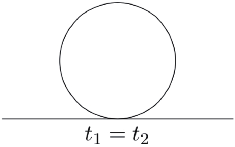
Figure 2. Tadpole diagram corresponding to
$ {\rm{Re}}\Pi^R.$ We observe that
$ \Pi_{12} = 0 $ because$ t_1 $ and$ t_2 $ must be identical. Using Eq. (2), we obtain$ \begin{split} \Pi^{R}(t_1,t_2) =& \Pi_{11}(t_1,t_2)\\ =& \frac{1}{2}\delta(t_1-t_2)\sum\limits_{\xi = \eta,\chi}\left[g_{\xi}\int \frac{{\rm d}^3p}{(2\pi)^3}(\Delta_\xi)_{11}({{p}},t_1,t_2)\right]\\ =& \frac{1}{2}\delta(t_1-t_2)\sum\limits_{\xi = \eta,\chi}\left[g_{\xi}\int \frac{{\rm d}^3p}{(2\pi)^3}{\rm{Re}}(\Delta_\xi)_>({{p}},t_1,t_2)\right]\; , \end{split} $

(20) with
$ g_{\eta}\equiv\lambda, g_{\chi}\equiv h $ . The integral is computed in Appendix C using the formulae in Appendix B.1,$ \Pi^R(t_1,t_2) = \delta(t_1-t_2)\left\{\frac{1}{2\pi^2\beta(t_1)^2}\sum\limits_{\xi = \eta,\chi}g_{\xi}h_3 \left[M_\xi\beta(t_1)\right]\right\}\; . $

(21) $ M_{\eta} $ and$ M_{\chi} $ denote the effective masses for η and χ, respectively, and$ h_3 $ is given by$ \begin{split} h_3(y) =& \frac{\pi^2}{12}-\frac{\pi y}{4}-\left(\frac{\gamma_E}{8}-\frac{1}{16}\right)y^2-\frac{y^2}{8}\log\frac{y}{4\pi}\\ & +\sum\limits_{m = 1}^{\infty}\frac{(-1)^{m+1}}{2^{m+3}}\frac{(2m-1)!!}{(m+1)!}\frac{\zeta(2m+1)}{(2\pi)^{2m}}y^{2m+2}\; , \end{split}$

(22) with
$ \gamma_E $ depicting the Euler constant. Fourier transforming Eq. (21) yields$ \begin{split} {\kappa}(t_1) =& \frac{1}{2\pi^2\beta(t_1)^2}\sum\limits_{\xi = \eta,\chi}g_{\xi}h_3\left[M_\xi\beta(t_1)\right]\\ \approx & \frac { \lambda + h } { 24 \gamma ^ { 2 } } \left( 1 - 2 H t _ { 1 } \right), \end{split}$

(23) where the final approximation corresponds to keeping only the first term of Eq. (22) and
$ \beta(t_1)^{-2} = \gamma^{-2} a(t_1)^{-2}\approx $ $\gamma^{-2}(1-2Ht_1) $ .As indicated in the Appendix C, the expansion in H brings in an extra divergent part in the integrals for the tadpole diagram. In this case, the
$ C_2 $ integral can be related to$ C_1 $ in a linear manner and therefore also vanishes. We can also use another scheme to perform the regularization such as the dimensional regularization scheme, which we employed when calculating$ \tilde{\kappa} $ in the next subsection. In fact, Ref. [47] proves that renormalization on curved backgrounds can be done in close analogy to renormalization in the Minkowski space, and that the removal of singularities follows the well-known power counting rules. This result is as expected, since the ultraviolet behaviour on smooth manifolds should be essentially identical to that in the Minkowski space. However, with two major obstacles, the infrared behavior and the absence of translation invariance, the curvature effects on the renormalization may be technically different and more complicated than the renormalization in flat spacetime, whereas the principle and the method are in close analogy. -
The leading order contribution to
$ \widetilde{\Pi}_R(t_1,t_2) $ and$ \widetilde{\kappa} (t_1)\equiv \widetilde{\kappa}(t_1,\omega = 0) $ is obtained from the "fish" diagram shown in Fig. 3, with the internal lines corresponding to two η or two χ free propagators: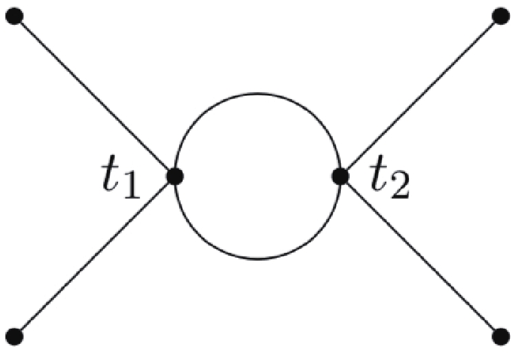
Figure 3. Fish diagram corresponding to
$ \widetilde{\Pi}^R.$ $ \begin{split} & \widetilde{\Pi}_R(t_1,t_2) = \widetilde{\Pi}_{11}(t_1,t_2)-\widetilde{\Pi}_{12}(t_1,t_2) \\ =& \frac{\rm i}{2}\sum\limits_{\xi = \eta,\chi}\int(-{\rm i}g_\xi)^2\frac{{\rm d}^3q}{(2\pi)^3}\Big[(\Delta_\xi)_{11} ({{q}},t_1,t_2)(\Delta_\xi)_{11}(-{{q}},t_1,t_2)\\ & -(\Delta_\xi)_{12}({{q}},t_1,t_2)(\Delta_\xi)_{12}(-{{q}},t_1,t_2)\Big]\\ =& \theta(t_1-t_2)\sum\limits_{\xi = \eta,\chi}g_{\xi}^{2}\int\frac{{\rm d}^3q}{(2\pi)^3}{\rm{Im}} \left[(\Delta_\xi)_>({{q}},t_1,t_2)^2\right]. \end{split} $

(24) To perform the integral over the three-momentum and carry out the Fourier transformation over
$ t = t_1-t_2 $ , we first expand the integrand in Eq. (24) to the first order in H,$ \begin{split} (\Delta_{\xi})_>({{q}},t_1,t_2)^2 \approx & \frac{1}{4\omega_{\xi q}^{2}}\left[(1-2Ht_1\overline{\gamma}_0)+Ht\overline{\gamma}_1\right.\\&\left.+2{\rm i}Ht_1t\overline{\gamma}_2-{\rm i}Ht^2\overline{\gamma}_2\right]\left(1+f\left(\omega_{\xi q}\right)\right)^2{\rm e}^{-2{\rm i}\omega_{\xi q} t}\\ &+(\omega_{\xi q}\to -\omega_{\xi q})-\frac{1}{2\omega_{\xi q}^2}\left[(1+Ht_1\gamma'_0)+Ht\gamma'_1\right]\\&\times(1+f(\omega_{\xi q}))f(\omega_{\xi q}), \end{split} $

(25) where
$ \omega_{\xi q} = \sqrt{{{q}}^2+M_\xi^2} $ and$ \left\{ \begin{split} &\overline{\gamma}_0(\omega_{\xi q}) = 3+\frac{\gamma M_\xi^2}{\omega_{\xi q}}f(\omega_{\xi q})-\frac{\omega_{\xi q}^2-M_\xi^2}{\omega_{\xi q}^2}\\ &\overline{\gamma}_1(\omega_{\xi q}) = 3+2\frac{\gamma M_\xi^2}{\omega_{\xi q}}f(\omega_{\xi q})-\frac{\omega_{\xi q}^2-M_\xi^2}{\omega_{\xi q}^2}\\ &\overline{\gamma}_2\left(\omega_{\xi q}\right) = \frac{\omega_{\xi q}^2-M_\xi^2}{\omega_{\xi q}}\\ &\gamma'_0(\omega_{\xi q}) = -6+2\frac{\omega_{\xi q}^2-M_\xi^2}{\omega^2_{\xi q}}-\left(1+2f(\omega_{\xi q})\right)\frac{\gamma M_\xi^2}{\omega_{\xi q}}\\ & \gamma'_1(\omega_{\xi q}) = 3+\frac{\gamma M_\xi^2}{\omega_{\xi q}}\left(1+2f(\omega_{\xi q})\right)-\frac{\omega^2_{\xi q}-M_\xi^2}{\omega_{\xi q}^2} \end{split} \right. \; . $

(26) For a general function K, given by
$ K = K_0(\omega_{\xi q}) + t K_1(\omega_{\xi q}) +t^{2} K_2(\omega_{\xi q}) $

(27) with
$ K_0(\omega_{\xi q}) $ ,$ K_1(\omega_{\xi q}) $ ,$ K_2(\omega_{\xi q}) $ being generic rational functions of$ \omega_{\xi q} $ , we obtain an explicit expression of its Fourier transformation in Appendix B.2:$ \begin{split}& {\rm{Re}} F^{\omega}\bigg[ \theta(t) {\rm{Im}} \int \frac{{\rm d}^{3} q}{(2 \pi)^{3}}\left[K_{0}\left(\omega_{{\xi q}}\right)+t K_{1}\left(\omega_{{\xi q}}\right)\right.\\ & \left.+t^{2} K_{2}\left(\omega_{{\xi q}}\right)\right] {\rm e}^{-2{\rm i} \omega_{{\xi q}} t}\bigg]\\ =& \left.I_{\rm re}\left[K_{0}\right]\right|_{\alpha_\xi = 0}+\frac{\partial}{\partial \omega} \left.I_{\rm im}\left[K_{1}\right]\right|_{\alpha_\xi = 0}-\frac{\partial^{2}}{\partial \omega^{2}} \left.I_{\rm re}\left[K_{2}\right]\right|_{\alpha_\xi = 0}\; , \end{split} $

(28) where
$ \alpha_\xi $ , which will be defined and used in the following section, is related to the decay rate of a ξ field.$ I_{\rm r e}\left[K\left(\omega_{{\xi q}}\right)\right] $ , and$ I_{\rm im}\left[K\left(\omega_{{\xi q}}\right)\right] $ are given as follows,$ \left\{ \begin{split} I_{\rm re}\left[K\left(\omega_{{\xi q}}\right)\right] =& \frac{1}{(2 \pi)^{3}} \int_{M_\xi}^{\infty} {\rm d} \omega_{{\xi q}} 4 \pi \omega_{{\xi q}} \sqrt{\omega_{{\xi q}}^{2}-M_\xi^2}\Bigg\{{\rm{Re}} K\left(\omega_{{\xi q}}\right) \frac{2 \omega_{{\xi q}}}{\omega^{2}-4 \omega_{{\xi q}}^{2}} +{\rm{Im}} K\left(\omega_{{\xi q}}\right)\Bigg[\frac{\alpha_\xi}{2\omega_{{\xi q}}\left(\omega+2 \omega_{{\xi q}}\right)^{2}}+\frac{\alpha_\xi}{2\omega_{{\xi q}}\left(\omega-2 \omega_{{\xi q}}\right)^{2}}\Bigg]\Bigg\}\; ,\\ I_{\rm im}\left[K\left(\omega_{{\xi q}}\right)\right] =& \frac{1}{(2 \pi)^{3}} \int_{M_\xi}^{\infty} {\rm d} \omega_{{\xi q}} 4 \pi \omega_{{\xi q}} \sqrt{\omega_{{\xi q}}^{2}-M_\xi^2}\Bigg\{{\rm{Im}} K\left(\omega_{{\xi q}}\right) \frac{\omega}{\omega^{2}-4 \omega_{{\xi q}}^{2}} -{\rm{Re}} K\left(\omega_{{\xi q}}\right)\Bigg[\frac{\alpha_\xi}{2\omega_{{\xi q}}\left(\omega-2 \omega_{{\xi q}}\right)^{2}}-\frac{\alpha_\xi}{2\omega_{{\xi q}}\left(\omega+2 \omega_{{\xi q}}\right)^{2}}\Bigg]\Bigg\}\; . \end{split} \right. $

(29) Combining Eq. (25) and Eq. (29), we obtain,
$ \begin{split} & \sum\limits_{\xi}g_\xi^2{\rm{Re}} F^{\omega} \left[\theta(t) {\rm{Im}} \int \frac{{\rm d}^{3} q}{(2 \pi)^{3}} (\Delta_{\xi})_>({{q}},t_1,t_2)^2\right]\\ =& \frac{1}{2}\sum\limits_{\xi}g_{\xi}^2\left\{I_{\rm re}\left[ \frac{1}{2\omega_{\xi q}^{2}}(1-2Ht_1\overline{\gamma}_0(\omega_{\xi q}))\left(1+f(\omega_{\xi q})\right)^2 -\frac{1}{2\omega_{\xi q}^{2}}(1-2Ht_1\overline{\gamma}_0(-\omega_{\xi q}))\left(1+f(-\omega_{\xi q})\right)^2 \right]\right.\\ &+\frac{\partial}{\partial \omega}I_{\rm im}\left[ \frac{H}{2\omega_{\xi q}^{2}}(\overline{\gamma}_1(\omega_{\xi q})+2{\rm i}t_1\overline{\gamma}_2(\omega_{\xi q}))\left(1+f(\omega_{\xi q})\right)^2 +\frac{H}{2\omega_{\xi q}^{2}}(-\overline{\gamma}_1(-\omega_{\xi q})+2{\rm i}t_1\overline{\gamma}_2(-\omega_{\xi q}))\left(1+f(-\omega_{\xi q})\right)^2 \right]\\ & \left.+\frac{\partial^2}{\partial \omega^2}I_{\rm re}\left[ {\rm i}H \frac{1}{2\omega_{\xi q}^{2}}\overline{\gamma}_2(\omega_{\xi q})\left(1+f(\omega_{\xi q})\right)^2 +{\rm i}H \frac{1}{2\omega_{\xi q}^{2}}\overline{\gamma}_2(-\omega_{\xi q})\left(1+f(-\omega_{\xi q})\right)^2 \right]\right\}\; . \end{split} $

(30) Setting
$ \omega = 0 $ and performing the integrals, we arrive at$ \begin{split}\tilde{\kappa}(t_1) = & \sum\limits_{\xi}g_\xi^2{\rm{Re}} F^{\omega} \left[\theta(t) {\rm{Im}} \int \frac{{\rm d}^{3} q}{(2 \pi)^{3}} (\Delta_{\xi})_>({{q}},t_1,t_2)^2\bigg|_{\omega = 0}\right]\\ =& -\sum\limits_{\xi = \eta,\chi}g_{\xi}^{2}(1-4Ht_1)\frac{1}{32\pi M_\xi\gamma}\; . \end{split} $

(31) If we set
$ H = 0 $ , we obtain the familiar results in flat spacetime,$ {\widetilde{\kappa}}(t_1)\approx -\frac{\lambda^2T}{32\pi M_{\eta}}-\frac{h^2T}{32\pi M_{\chi}}\; , $

(32) using the Minkowski-space propagators in loop diagrams.
-
As mentioned in Ref. , the leading contribution to
$ \left.\frac{\partial }{\partial \omega} {\widetilde{\kappa}}(t_1,-\omega)\right|_{\omega = 0} $ comes from the fish diagram, Fig. 3, but with the one-loop corrected ($ \eta- $ or$ \chi- $ ) propagators. Such propagators rely on the decay rates, which were calculated in Ref. in flat spacetime:$ \Gamma_{\chi} = \frac{\lambda'^2+3h^2}{256\pi^3\gamma^2\omega_{\chi}}\equiv \frac{\alpha_{\chi}}{\omega_{\chi}}, \, \Gamma_{\eta} = \frac{\lambda^2+3h^2}{256\pi^3\gamma^2\omega_{\eta}}\equiv \frac{\alpha_{\eta}}{\omega_{\eta}}. $

(33) In the present situation, as we assumed the system to be in pseudo-equilibrium, and we do not consider higher order corrections, we replace Eq. (33) by
$ \Gamma_{\chi}(t') = \frac{\lambda'^2+3h^2}{256\pi^3\beta(t')^2\Omega_{\chi}(t')}\; , \, \Gamma_{\eta}(t') = \frac{\lambda^2+3h^2}{256\pi^3\beta(t')^2\Omega_{\eta}(t')}\; . $

(34) Similar to Eq. (28), we have
$ \begin{split} & F^{\omega}\left[\theta(t) {\rm{Im}} \int \frac{{\rm d}^{3} q}{(2 \pi)^{3}}\left(K_{0}+t K_{1}+t^{2} K_{2}\right) {\rm e}^{- \frac{\alpha_\xi}{\omega_{q}} t}\right]\\ =& \int \frac{{\rm d}^3q}{(2\pi)^3}\left({\rm{Im}}K_0\frac{\omega_q \alpha_\xi}{\alpha_\xi^2+\omega^2\omega^2_q}+{\rm{Im}}K_1\frac{\partial}{\partial \omega}\frac{\omega\omega^2_q}{\alpha_\xi^2+\omega^2\omega^2_q}\right.\\&\left.-{\rm{Im}}K_2\frac{\partial^2}{\partial \omega^2}\frac{\omega_q \alpha_\xi}{\alpha_\xi^2+\omega^2\omega^2_q}\right) +{\rm i}\int \frac{{\rm d}^3q}{(2\pi)^3}\left({\rm{Im}}K_0\frac{\omega\omega^2_q}{\alpha_\xi^2+\omega^2\omega^2_q}\right.\\&\left.-{\rm{Im}}K_1\frac{\partial }{\partial \omega}\frac{\omega_q\alpha_\xi}{\alpha_\xi^2+\omega^2\omega^2_q}-{\rm{Im}}K_2\frac{\partial ^2}{\partial \omega^2}\frac{\omega\omega^2_q}{\alpha_\xi^2+\omega^2\omega^2_q}\right) \end{split} $

(35) and
$\begin{split} &{\rm{Im}} F^{\omega} \left\{\theta(t) {\rm{Im}} \int \frac{{\rm d}^{3} q}{(2 \pi)^{3}}\left[K_{0}\left(\omega_{{\xi q}}\right)\right.\right.\\&\left.\left.+t K_{1}\left(\omega_{{\xi q}}\right)+t^{2} K_{2}\left(\omega_{{\xi q}}\right)\right] {\rm e}^{-2 {\rm i} \omega_{{\xi q}} t}\right\}\\ =& I_{\rm i m}\left[K_{0}\right]-\frac{\partial}{\partial \omega} I_{\rm r e}\left[K_{1}\right]-\frac{\partial^{2}}{\partial \omega^{2}} I_{\rm i m}\left[K_{2}\right], \end{split} $

(36) where
$ I_{\rm re} $ and$ I_{\rm im} $ are defined in Eq. (29), and the derivation of which is provided in Appendix B.2. By expanding the propagator to the first order in H and making the following peak approximation,$ f(\omega_{\xi q})\to \frac{1}{\gamma \omega_{\xi q}}, \int_{m}^{\infty}\to \int_{m}^{1/\gamma}, $

(37) and subsequently with the help of Eq. (35) and Eq. (36) to perform the Fourier transformations, to the first order in H and to the lowest orders in
$ \alpha_{\chi} $ and$ \alpha_{\eta} $ , we obtain$ \begin{split}-{\rm i} \left.\frac{\partial }{\partial \omega} {\widetilde{\kappa}}(t_1,-\omega)\right|_{\omega = 0} = & -h^2\left[-\frac{32\pi\gamma}{\lambda'^2+3h^2}\left(1+\log\frac{M_{\chi}\gamma}{2}\right)+Ht_1\frac{32\pi\gamma}{3\left(\lambda'^2+3h^2\right)}\left(5+9\log\frac{M_{\chi} \gamma}{2}\right)-H\frac{2^{13}\pi^4\gamma^2}{\left(\lambda'^2+3h^2\right)^2}\right]\\ & -\lambda^2\left[-\frac{32\pi\gamma}{\lambda^2+3h^2}\left(1+\log\frac{M_{\chi}\gamma}{2}\right)+Ht_1\frac{32\pi\gamma}{3\left(\lambda^2+3h^2\right)}\left(5+9\log\frac{M_{\chi}\gamma}{2}\right)-H\frac{2^{13}\pi^4\gamma^2}{\left(\lambda^2+3h^2\right)^2}\right]\; . \end{split} $

(38) -
$ \left.\frac{\partial }{\partial \omega} {\kappa}(t_1,-\omega)\right|_{\omega = 0} $ is determined by the imaginary part of the self-energy , whose leading order contribution for soft momenta comes from the sunset diagram in Fig. 4.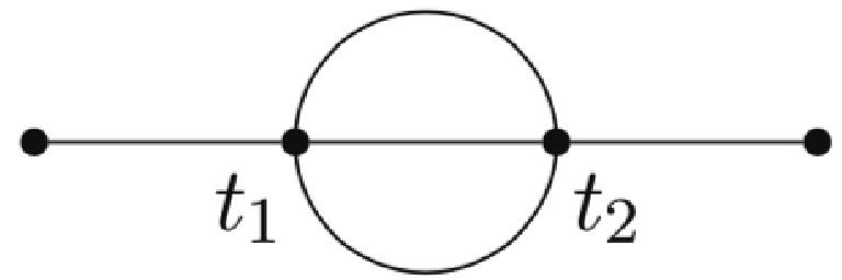
Figure 4. Sunset diagram corresponding to
$ {\rm{Im}}\Pi^R$ .$ \begin{split} \Pi^R(t_1,t_2) =& h^2\theta(t_1-t_2)\int \frac{{\rm d}^3 k}{(2\pi)^3}\frac{{\rm d}^3l}{(2\pi)^3}{\rm{Im}}\left[(\Delta_{\chi})_>({{k}},t_1,t_2)\right.\\ &\left.\times(\Delta_{\chi})_>({{l}},t_1,t_2)(\Delta_{\eta})_>({{k}}+{{l}},t_1,t_2)\right]\; . \end{split} $

(39) In Appendix D, we show that we can express the derivative of
$ \kappa(-\omega) $ in the following form, where the derivatives of$ I_s, I_c, J_s, J_c $ are given by equations (102), (103), (105), (106),$ \begin{split} -{\rm i} \left.\frac{\partial }{\partial \omega} {\kappa}(t_1,-\omega)\right|_{\omega = 0} =& -\frac{h^2}{8}\Bigg\{ \left( 1 - 9 H t _ { 1 } \right) \left. \frac { \partial } { \partial \omega } I _ { s } \left[ \gamma _ { 0 } \right] \right| _ { \omega = 0 } + H t _ { 1 }\left. \frac { \partial } { \partial \omega } I _ { s } \left[ \gamma _ { 1 } \right] \right| _ { \omega = 0 } - H t _ { 1 }\left. \frac { \partial } { \partial \omega } I _ { s } \left[ \gamma _ { 2 } \right] \right| _ { \omega = 0 } - 2 H t _ { 1 }\left. \frac { \partial ^ { 2 } } { \partial \omega ^ { 2 } } I _ { c } \left[ \gamma _ { 3 } \right] \right|_ { \omega = 0 }\\ & -\frac { 9 } { 2 } H\left. \frac { \partial } { \partial \omega } J _ { s } \left[ \gamma _ { 0 } \right] \right| _ { \omega = 0 } - \frac { 1 } { 2 } H \left. \frac { \partial } { \partial \omega } J _ { s } \left[ \gamma _ { 1 } \right] \right|_ { \omega = 0 } + H \left. \frac { \partial } { \partial \omega } J _ { s } \left[ \gamma _ { 2 } \right] \right| _ { \omega = 0 } - H\left. \frac { \partial } { \partial \omega } J _ { c } \left[ \gamma _ { 3 } \right] \right|_ { \omega = 0 }\Bigg\}\; . \end{split} $

(40) Here, the
$ \gamma_i $ are the new ones defined in Appendix D. This derivation is not significantly different from the calculation of the imaginary part of the self-energy performed in Ref. . However, the analogous integrals in de Sitter spacetime are more complicated: we do not have our disposal the delta functions, resulting from the momentum conservation, to simplify the calculations. Our strategy is to calculate each term in the above equation, with the assumption that$ M_{\chi}/M_{\eta}\ll 1 $ , to obtain analytical results of the integrals.Let us now calculate the first line in the curly bracket in Eq. (40), which is dominated by regions where
$ \omega_{\chi k},\omega_{\chi l}\ll 1/\gamma $ , since in these regions the Bose distribution function contains a peak. In this subsection, we expand the Bose distribution function to$ O((1/\gamma)^0) $ ,$ f(x)\approx 1/(\gamma x)-1/2 \quad ({\rm{for }}\quad x\ll 1/\gamma) $ , to simplify the integrals, because the contributions from$ 1/(\gamma x) $ to some of the results (e.g., the second line in the curly bracket in Eq. (40)) will vanish due to cancellations of terms with opposite signs. Because$ \gamma_0,\gamma_1,\gamma_2 $ (at least to the zeroth order in$ M_{\eta}\gamma $ ) do not change when all three arguments change simultaneously, while$ \gamma_3 $ changes sign, the temperature-dependent part in$ \partial /\partial \omega I_s[\gamma_{0,1,2}]|_{\omega = 0} $ and in$ \partial^2 /\partial^2 \omega I_c[\gamma_3] |_{\omega = 0} $ appears in the following forms:$ \begin{split} & \left(1+f(\omega_{\eta q})\right)f(\omega_{\chi k})f(\omega_{\chi l})-f(\omega_{\eta q})\left(1+f(\omega_{\chi k})\right)\left(1+f(\omega_{\chi l})\right)\\ & \approx \frac{1}{\gamma^2}\left(\frac{1}{\omega_{\chi k}\omega_{\chi l}}-\frac{1}{\omega_{\eta q}\omega_{\chi k}}-\frac{1}{\omega_{\eta q}\omega_{\chi l}}\right),\\ &\left(1+f(\omega_{\eta q})\right)f(\omega_{\chi k})f(\omega_{\chi l})+f(\omega_{\eta q})\left(1+f(\omega_{\chi k})\right)\left(1+f(\omega_{\chi l})\right)\\ & \approx \frac{2}{\gamma^3\omega_{\eta q}\omega_{\chi k}\omega_{\chi l}}\; . \end{split} $

(41) We thus conclude that
$ \partial /\partial \omega I_s[\gamma_{0,1,2}]|_{\omega = 0} $ is considerably smaller than$ \partial^2 /\partial^2 \omega I_c[\gamma_3] |_{\omega = 0} $ , and the former can be safely neglected.Considering
$ - \left. \dfrac { \partial ^ { 2 } } { \partial \omega ^ { 2 } } I _ { c } \left[ \gamma _ { i } \right] \right|_ { \omega = 0 } $ , it is the sum of the following three integrals Eq. (103),$ \begin{split}&- \frac { 1 } { 2 ( 2 \pi ) ^ { 3 } } \int _ { M_{\chi} } ^ { \infty } {\rm d} \omega_{\chi l}\int _ { M_{\chi} t _ { 0 m } } ^ { M_{\chi} t _ { 0 p } } {\rm d} \omega_{\chi k} \frac { \partial ^ { 2 } } { \partial \omega ^ { 2 } }\Big[\gamma _ { i } \left( - \omega + \omega_{\chi k} + \omega_{\chi l}- \omega_{\chi k} , - \omega_{\chi l} \right) \left( 1 + f \left( \omega_{\chi k} + \omega_{\chi l} - \omega \right) \right) f \left( \omega_{\chi k} \right) f \left( \omega_{\chi l} \right)\\ & \quad - \gamma _ { i } \left( \omega - \omega_{\chi k} - \omega_{\chi l} , \omega_{\chi k} , \omega_{\chi l} \right) f \left( \omega_{\chi k} + \omega_{\chi l} - \omega \right) \left( 1 + f \left( \omega_{\chi k} \right) \right) \left( 1 + f \left( \omega_{\chi l} \right) \right)\Big]\bigg|_{\omega = 0}, \end{split} $

(42) $ \begin{split} &- \frac { 1 } { 2 ( 2 \pi ) ^ { 3 } } \int _ { M_{\chi} } ^ { \infty } {\rm d} \omega_{\chi l}M_{\chi}^2(t_{1p})^2\frac{\partial}{\partial \omega_{\chi k}}\Big[\gamma_i(\omega_{\chi k}+\omega_{\chi l},-\omega_{\chi k},-\omega_{\chi l})\left(1+f\left(\omega_{\chi k}+\omega_{\chi l}\right)\right)f\left(\omega_{\chi k}\right)f\left(\omega_{\chi l}\right)\\ & \quad -\gamma_i\left(-\omega_{\chi k}-\omega_{\chi l},\omega_{\chi k},\omega_{\chi l}\right)f\left(\omega_{\chi k}+\omega_{\chi l}\right)\left(1+f\left(\omega_{\chi k}\right)\right)\left(1+f\left(\omega_{\chi l}\right)\right)\Big]\bigg|_{\omega_{\chi k}\to M_{\chi} t_{0p}}, \end{split}$

(43) $ \begin{split}&\frac { 1 } { 2 ( 2 \pi ) ^ { 3 } } \int _ { M_{\chi} } ^ { \infty } {\rm d} \omega_{\chi l}M_{\chi}^2(t_{1m})^2\frac{\partial}{\partial \omega_{\chi k}}\Big[\gamma_i(\omega_{\chi k}+\omega_{\chi l},-\omega_{\chi k},-\omega_{\chi l})\left(1+f\left(\omega_{\chi k}+\omega_{\chi l}\right)\right)f\left(\omega_{\chi k}\right)f\left(\omega_{\chi l}\right)\\ & \quad -\gamma_i\left(-\omega_{\chi k}-\omega_{\chi l},\omega_{\chi k},\omega_{\chi l}\right)f\left(\omega_{\chi k}+\omega_{\chi l}\right)\left(1+f\left(\omega_{\chi k}\right)\right)\left(1+f\left(\omega_{\chi l}\right)\right)\Big]\bigg|_{\omega_{\chi k}\to M_{\chi} t_{0m}}\; . \end{split} $

(44) $ M_{\chi} t_{0p} $ grows rapidly with$ \omega_{\chi l} $ :$ M_{\chi} t_{0p}\sim\frac{M_{\eta}^2}{M_{\chi}^2}\omega_{\chi l} $ , while$ M_{\chi} t_{0m} $ decreases with$ \omega_{\chi l} $ . Therefore, for the integral Eq. (43), the rational-function approximation of the Bose distribution function is inappropriate. The integrand will indeed be negligible due to the large exponential in the denominator. In contrast, it is viable to use the rational-function approximation in the integral Eq. (44), which turns out to be significantly larger than Eq. (43). For the integral Eq. (42), we see that there. is no significant difference in the order of magnitude if we replace the partial derivative$ \partial /\partial \omega $ by$ \partial /\partial \omega_{\chi k} $ . After carrying out this replacement, it can be written as$ [(43)/(M_{\chi}t_{1p})^2-(44)/(M_{\chi}t_{1m})^2] $ . The first term can be neglected, because Eq. (43) is small, and$ M_{\chi}t_{1p} $ is large. We can also neglect the second term, because$ M_{\chi}t_{1m} $ is significantly greater than 1 when$ \omega_{\chi l} $ is small, and we can make a rough estimate of the ratio of the contribution of$ M_{\chi}t_{1m} $ to that of 1,$ \dfrac{ \displaystyle\int_{M_{\chi}}^{M_{\eta}}M_{\chi}t_{1m}{\rm d}\omega_{\chi l}}{ \displaystyle\int_{M_{\chi}}^{M_{\eta}}{\rm d}\omega_{\chi l}}\approx \frac{M_{\eta}}{6M_{\chi}}\; . $

(45) Eq. (42) is indeed significantly smaller than Eq. (44), and therefore we only keep Eq. (44).
Upon performing the approximations above, Eq. (103) can be integrated,
$ \begin{split} - \left. \frac { \partial ^ { 2 } } { \partial \omega ^ { 2 } } I _ { c } \left[ \gamma _ { 3} \right] \right|_ { \omega = 0 } \approx & \frac { 1 } { ( 2 \pi ) ^ { 3 } }\int _ { M_{\chi} } ^ { \infty } {\rm d} \omega_{\chi l}M_{\chi} ^ { 2 } \left( t _ { 1 m } \right) ^ { 2 } \frac { \partial } { \partial \omega_{\chi k} } \left[ \gamma _ { 3 } \left( \omega_{\chi k} + \omega_{\chi l} , - \omega_{\chi k} , - \omega_{\chi l} \right)\frac{1}{\gamma^3\left(\omega_{\chi k}+\omega_{\chi l}\right)\omega_{\chi k}\omega_{\chi l}}\right]\bigg|_{\omega_{\chi k}\to M_{\chi} t_{0m}}\\ \approx & \frac{T^3}{4\pi^3M_{\eta}^2}\left[\frac{M_{\eta}^8}{(M_{\eta}^4+4M_{\chi}^2T^2)^2}-\frac{M_{\eta}^4}{M_{\eta}^4+4M_{\chi}^2T^2}-\frac{4M_{\chi}^2M_{\eta}^4T^2}{(M_{\eta}^4+4M_{\chi}^2T^2)^2}+\frac{8M_{\chi}^4T^2}{M_{\eta}^2(M_{\eta}^4+4M_{\chi}^2T^2)}\right.\\ & \left.+\log\left(\frac{1}{4}\right)-1+\log\left(\frac{M_{\eta}^6}{M_{\chi}^4\sqrt{M_{\eta}^4+4M_{\chi}^2T^2}}\right)\right]\; . \end{split} $

(46) This analytic result is evaluated for a few pairs of
$ ( M_{\chi}, M_{\eta}) $ , and their values are compared with results obtained by numerical integration for a few pairs of$ ( M_{\chi}, M_{\eta}) $ . The accuracy of this approximation is found to be within 5%, as shown in Table 1.T $ M_{\eta} $ 

$ M_{\chi} $ 

analytic result numerical result error $ 1\times 10^5 $ 

$ 500 $ 

1 $7.01\times10^{8}$ 

$ 7.30\times10^8 $ 

−4% $ 1\times 10^5 $ 

$ 1000 $ 

1 $ 2.03\times 10^8 $ 

$ 1.99\times 10^8 $ 

2% $ 1\times 10^4 $ 

$ 100 $ 

1 $ 1.20\times 10^7 $ 

$ 1.19\times 10^7 $ 

0.9% $ 1\times 10^4 $ 

$ 100 $ 

0.5 $ 1.45\times 10^7 $ 

$ 1.51\times 10^7 $ 

−3.8% Table 1. Analytical result Eq. (46) obtained under approximation
$ M_{\eta}\gg M_{\chi} $ , evaluated for a few pairs of$( M_{\chi}, M_{\eta})$ . The integral (first line in the curly bracket in Eq. (40)) is performed by numerical integration, and final values are evaluated for same set of$( M_{\chi}, M_{\eta})$ . The accuracy of the approximation,$ M_{\eta}\gg M_{\chi} $ , is found to be within 5%.Next, we compute
$ \partial /\partial \omega J_c[\gamma_3]|_{\omega = 0} $ and$ \partial /\partial \omega J_s[\gamma_{0,1,2}]|_{\omega = 0} $ , where we assume that$ \lambda, \lambda', h\ll M_{\chi} \gamma $ . As we mentioned in Section 2, for the calculations to be carried out perturbatively,$ \lambda,\lambda', h $ should be sufficiently small and in particular smaller than any dimensionless quantity that can be constructed using dimensionful dynamical quantities in the model. There are eight terms in$ \partial /\partial \omega J_c[\gamma_i]|_{\omega = 0} $ , with different signs$ \chi_q,\chi_k,\chi_l $ before$ \omega_{\eta q},\omega_{\chi k},\omega_{\chi l} $ . We first compute the terms in$ \partial /\partial \omega J_c[\gamma_3]|_{\omega = 0} $ that correspond to$ \chi_q = 1,\chi_k = -1,\chi_l = -1 $ and$ \chi_q = -1,\chi_k = 1,\chi_l = 1 $ :$ \begin{split}& 6 \frac { 1 } { ( 2 \pi ) ^ { 4 } } \int _ { M_{\chi} } ^ { \infty } {\rm d} \omega_{\chi k} {\rm d} \omega_{\chi l} \int _ { - 1 } ^ { 1 } {\rm d} w \frac { \sqrt { \omega_{\chi k} ^ { 2 } - M_{\chi} ^ { 2 } } \sqrt { \omega_{\chi l} ^ { 2 } - M_{\chi} ^ { 2 } } \left( \omega _ { \eta q } -\omega_{\chi k} - \omega_{\chi l} \right) ^ 4} { \omega _ { \eta q } \left[\left( \omega _ { \eta q } - \omega_{\chi k} - \omega_{\chi l} \right) ^2+\alpha_{\chi}^2\left(1/(2\omega_{\chi k})+1/(2\omega_{\chi l})\right)^2\right] ^4} \gamma _ { 3} \left( \omega _ { \eta q } , -\omega_{\chi k} , -\omega_{\chi l} \right)\\ & \times [(1+f(\omega_{\eta q}))(1+f(-\omega_{\chi k}))(1+f(-\omega_{\chi l}))+(1+f(-\omega_{\eta q}))(1+f(\omega_{\chi k}))(1+f(\omega_{\chi l}))]\; , \end{split} $

(47) here, the integration variable
$ w = \dfrac{ {{k}} \cdot {{l}} }{ k\, l} $ is the cosine of the angle between two momenta k and l.These are the dominant contribution to the principle part of the sunset diagram. The second line in the above formula has a peak when
$ \omega_{\chi k},\omega_{\chi l}\ll 1/\gamma $ , allowing us to approximate it by$ \begin{split} & \frac{1}{12\omega_{\chi k}\omega_{\chi l}\omega_{\eta q}}\times\left[\omega_{\chi k}^{2}(\omega_{\eta q}-\omega_{\chi l})+\omega_{\chi l}^{2}(\omega_{\eta q}-\omega_{\chi k})\right.\\ & \left.-\omega_{\eta q}^{2}(\omega_{\chi k}+\omega_{\chi l})+3\omega_{\chi k}\omega_{\chi l}\omega_{\eta q}\right]+\frac{\omega_{\eta q}-\omega_{\chi k}-\omega_{\chi l}}{\gamma^2\omega_{\eta q}\omega_{\chi k}\omega_{\chi l}}\; , \end{split} $

(48) and to cut down the upper limit of integration to
$ 1/\gamma $ . The approximation is carried out to the order$ O(1/\gamma^0) $ since by calculation, it turns out that the$ O(1/\gamma^0) $ term has a greater order of contribution to the integral than the$ O(1/\gamma^2) $ term. This is due to the fact that the$ O(1/\gamma^2) $ term is proportional to$ \omega_{\eta q}-\omega_{\chi k}-\omega_{\chi l} $ , which is very small around the peak. Let us now consider the following term in the integral:$ G(\omega_{\chi k},\omega_{\chi l},w) = \frac{g(\omega_{\chi k},\omega_{\chi l},w)^4}{\left[g(\omega_{\chi k},\omega_{\chi l},w)^2+\alpha_{\chi}^2\left(\dfrac{1}{2\omega_{\chi k}}+\dfrac{1}{2\omega_{\chi l}}\right)^2\right]^4}, $

(49) where
$ \begin{split}&g(\omega_{\chi k},\omega_{\chi l},w) \equiv \omega_{\eta q}-\omega_{\chi k}-\omega_{\chi l}\\ =& \sqrt{\omega_{\chi k}^2+\omega_{\chi l}^2+2w\sqrt{\omega_{\chi k}^2-M_{\chi}^2}\sqrt{\omega_{\chi l}^2-M_{\chi}^2}+M_{\eta}^{2}-2M_{\chi}^2}\\ & -\omega_{\chi k}-\omega_{\chi l}. \\[-10pt] \end{split} $

(50) Since
$ \alpha_{\chi}/M_{\chi}^2\ll 1/(256\pi^3)\Rightarrow \alpha_{\chi}/M_{\chi}^2\ll 10^{-4} $ , one infers that G has a peak (see Fig. 5 for the plot of the integrand in Eq. (47)) around some points, where$ g(\omega_{\chi k},\omega_{\chi l},w) $ and$ \alpha_{\chi}(1/\omega_{\chi k}+1/\omega_{\chi l}) $ have the same order of magnitude. Hence,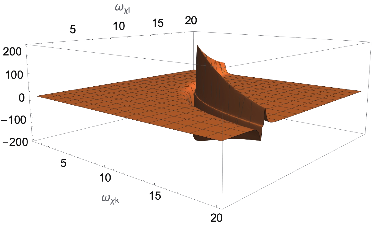
Figure 5. (color online) Plot of integrand in Eq. (47), where w is taken as -1 and
$ T = 1000, M_{\eta} = 20, M_{\chi} = 1$ .$ \begin{split} \omega_{\chi k}\omega_{\chi l} =& \frac{M_{\eta}^2}{2(1-w)}+O\left(M_{\chi}^2\right)+O\left(\alpha_{\chi}\right),\\ \omega_{\chi k},\omega_{\chi l} =& O(M_{\eta})+O\left(\frac{M_{\chi}^2}{M_{\eta}}\right) +O\left(\frac{\alpha_{\chi}}{M_{\eta}}\right). \end{split} $

(51) Furthermore, we note that if we vary
$ g(\omega_{\chi k},\omega_{\chi l}, w) $ by an amount of order$ \alpha_{\chi}/M_{\eta} $ , then$ \alpha_{\chi}(1/\omega_{\chi k}+1/\omega_{\chi l}) $ would vary by an amount of order$ \alpha_{\chi}^2/M_{\eta}^3 $ , i.e., the latter can be regarded as a constant. Hence, to determine the local maximum points of$ G(\omega_{\chi k},\omega_{\chi l},w) $ to an order of$ O(\alpha_{\chi}/M_{\eta}) $ , we require that$ g(\omega_{\chi k},\omega_{\chi l}, w) = \alpha_{\chi}\left(\frac{1}{2\omega_{\chi k}}+\frac{1}{2\omega_{\chi l}}\right)\; . $

(52) $ \omega_{\chi k}, \omega_{\chi l} $ are apparently symmetric in these formulae. To simplify the calculations, we define a set of new variables:$ \mu = \omega_{\chi k}+\omega_{\chi l}, \nu = \omega_{\chi k}\omega_{\chi l}/M_{\eta} $ . Then, Eq. (52) becomes$ g(\mu,\nu) = \frac{\alpha_{\chi}\mu}{2M_{\eta}\nu}, $

(53) and to the lowest order in
$ \alpha_{\chi}/M_{\eta} $ and$ M_{\chi}^2/M_{\eta} $ , the solution to the above equation is$ \nu_{\max} = \frac{M_{\eta}}{2(1-w)}\; . $

(54) We expand G near
$ \nu_{\max} $ , where G has a peak and thus the integration region becomes a band that is narrow in the ν direction and runs along the µ direction. From Eq. (51), we see that the width of the band can be chosen to be$ \alpha_{\chi}/M_{\chi} $ , since$ \alpha_{\chi}/M_{\chi}\gg \alpha_{\chi}/M_{\eta} $ . First we expand the function g around$ \nu_{\max} $ :$ \begin{split}&g\left(\mu,\nu_{\max}(\mu)+\Delta\right) = g\left(\mu,\nu_{\max}(\mu)\right)+\Delta\cdot \left.\frac{\partial g}{\partial \nu}\right|_{\mu,\nu_{\max}(\mu)}\\ = & \alpha_{\chi}\frac { \mu } { 2M_{\eta} \nu_ { \max } ( \mu ) } - \frac { M_{\eta} } { \mu } ( 1 - w ) \Delta-\frac{M_{\eta}^{2}}{2\mu^3}(1-w)^2\Delta^2\; . \end{split} $

(55) where we expanded to the second order in ∆, because as we later integrate over ∆, the integrand contains a term that is an odd funtion of g, and it is necessary to include the
$ O(\Delta^2) $ contribution to obtain a non-vanishing result. Inserting it into G, we have$\begin{split}& G \left( \mu , \nu_ { \max } ( \mu ) + \Delta \right) \\=& \frac { g \left( \mu , \nu_ { \max } ( \mu ) + \Delta \right) ^ { 4 } } { \left[ g \left( \mu , \nu_ { \max } ( \mu ) + \Delta \right) ^ { 2 } + \dfrac { \alpha_{\chi} ^ { 2 } \mu ^ { 2 } } { 4M _{\eta}^ { 2 } \nu_ { \max } ( \mu ) ^ { 2 } } \right] ^ { 4 } }, \end{split}$

(56) where we made an approximation:
$ \alpha_{\chi}^2 \mu^2/\left\{M_{\eta}^2\left[\nu_{\max}(\mu)+\Delta\right]^2\right\}\approx \alpha_{\chi}^2 \mu^2/\left[M_{\eta}^2\nu_{\max}(\mu)^2\right]. $

(57) We note that the dominant contribution of Eq. (48) comes from the
$ O((1/\gamma)^0) $ term. Expanding this term to the second order in$ (\omega_{\eta q}-\mu) $ , the integrand in Eq. (47) becomes$\begin{split}& 6 \frac { 1 } { ( 2 \pi ) ^ { 4 } }\frac { \sqrt { \omega_{\chi k} ^ { 2 } - M_{\chi} ^ { 2 } } \sqrt { \omega_{\chi l} ^ { 2 } - M_{\chi} ^ { 2 } } } { \omega _ { \eta q } } G \left( \mu , \nu _ { \max } ( \mu ) + \Delta \right)\\&\times\left( \frac { \omega _ { \eta q } ^ { 2 } - M_{\eta} ^ { 2 } } { 2 \omega _ { \eta q } } - \frac { 1 } { 2 } \mu + \frac { M_{\chi} ^ { 2 } \mu } { 2 M_{\eta} \nu} \right)\\&\times \left[-\frac{(\omega_{\eta q}-\mu)^2}{12\mu^2}-\frac{\mu^2-M_{\eta}\nu_{\max}(\mu)}{12M_{\eta}\nu_{\max}(\mu)\mu}(\omega_{\eta q}-\mu)\right]. \end{split}$

(58) By expanding Eq. (48) into the second order in g and taking into consideration that in the narrow band we have
$ \nu = \frac { M_{\eta} } { 2 ( 1 - w ) } + O \left( \frac { M_{\chi} ^ { 2 } } { M_{\eta} } \right) + O \left( \frac { \alpha_{\chi} } { M_{\eta} } \right) , $

$ \omega _ { \eta q } = \mu + g \left( \mu ,\nu _ { \max } ( \mu ) + \Delta \right), \quad $

Eq. (47) is determined by the following contribution to equation (58):
$ \begin{split}&6 \cdot \frac { 1 } { ( 2 \pi ) ^ { 4 } } \frac { M_{\eta} ^ { 2 } } { 2 ( 1 - w ) } \frac { 1 } { \mu } \left[ - \frac { M_{\eta} ^ { 2 } } { 2 \mu } + ( 1 - w ) \frac { M_{\chi} ^ { 2 } \mu } { M_{\eta} ^ { 2 } } \right] \frac { g \left( \mu , \nu _ { \max } ( \mu ) + \Delta \right) ^ { 4 } } { \left[ g \left( \mu , \nu _ { \max } ( \mu ) + \Delta \right) ^ { 2 } + \dfrac { \alpha_{\chi} ^ { 2 } \mu ^ { 2 } } { 4M_{\eta} ^ { 2 } \nu _ { \max } ( \mu ) ^ { 2 } } \right] ^ { 4 } }\\ &\quad \times \left[-g \left( \mu , \nu _ { \max } ( \mu ) + \Delta \right)^2\cdot \frac{1}{12\mu^2}-g \left( \mu , \nu _ { \max } ( \mu ) + \Delta \right)\frac{\mu^2-M_{\eta}\nu_{\max}(\mu)}{12M_{\eta}\nu_{\max}(\mu)\mu}\right]. \end{split} $

(59) Since outside of the band the integrand is negligible, the integration region of ∆ can be chosen to be
$ (-\infty,\infty) $ . We also have restrictions on the range of µ and w: in the band we have$ \begin{split} &{\mu ^2} = {\left( {{\omega _{\chi k}} + {\omega _{\chi l}}} \right)^2} \ge 4{\omega _{\chi k}}{\omega _{\chi l}} \approx \frac{{2M_\eta ^2}}{{1 - w}} \ge M_\eta ^2\\ \Rightarrow & (\mu \ge {M_\eta }){\rm{\& }}\left(w \le 1 - \frac{{2M_\eta ^2}}{{{\mu ^2}}}\right). \end{split}$

(60) Therefore, the measure becomes
$ \begin{split}&\int _ { - 1 } ^ { 1 } {\rm d} w \int _ { M_{\chi} } ^ { 1 / \gamma } {\rm d} \omega_{\chi k} \int _ { M_{\chi} } ^ { 1 / \gamma } {\rm d} \omega_{\chi l}\\ = & \int _ { - 1 } ^ { 1 - \frac { 2 M_{\eta} ^ { 2 } } { \mu ^ { 2 } } } {\rm d} w \int _ { M_{\eta} } ^ { 2 / \gamma } {\rm d} \mu \int _ { -\infty} ^ { \infty } {\rm d} \Delta \frac { M_{\eta} } { \sqrt { \mu ^ { 2 } - 4 M_{\eta} v } }. \end{split}$

(61) Hence, the integral Eq. (47) becomes
$ \begin{split}& 6 \cdot \frac { 1 } { ( 2 \pi ) ^ { 4 } } \int _ { M_{\eta} } ^ { 2 / \gamma } {\rm d} \mu \int _ { - 1 } ^ { 1 - \frac { 2 M_{\eta} ^ { 2 } } { \mu ^ { 2 } } } {\rm d} w \frac { M_{\eta} } { \sqrt { \mu ^ { 2 } - \dfrac { 2 M_{\eta} ^ { 2 } } { 1 - w } } } \frac { M_{\eta} ^ { 2 } } { 2 ( 1 - w ) } \frac { 1 } { \mu } \left[ - \frac { M_{\eta} ^ { 2 } } { 2 \mu } + ( 1 - w ) \frac { M_{\chi}^ { 2 } \mu } { M_{\eta} ^ { 2 } } \right]\\ & \times\left\{-\frac{1}{12\mu^2}\int _ { - \infty} ^ { \infty } {\rm d} \Delta\dfrac { \left[ \dfrac { 2M_{\eta} \nu _ { \max } ( \mu ) } { \alpha_{\chi} \mu } \right] ^ { 2 }\left[ 1 - \dfrac { 2( 1 - w ) M_{\eta} ^ { 2 } \nu _ { \max } ( \mu ) } { \alpha_{\chi} \mu ^ { 2 } } \Delta - \dfrac { ( 1 - w )^2 M _{\eta}^ { 3 } \nu _ { \max } ( \mu ) } { \alpha_{\chi} \mu ^ { 4 } } \Delta^2 \right] ^ { 6 } } { \left\{ \left[ 1 - \dfrac { 2( 1 - w ) M _{\eta}^ { 2 } \nu _ { \max } ( \mu ) } { \alpha_{\chi} \mu ^ { 2 } } \Delta - \dfrac { ( 1 - w )^2 M _{\eta}^ { 3 } \nu _ { \max } ( \mu ) } { \alpha_{\chi} \mu ^ { 4 } } \Delta^2\right] ^ { 2 } + 1 \right\} ^ { 4 } }\right.\\ &\left.-\frac{\mu^2-M_{\eta}\nu_{\max}(\mu)}{12M_{\eta}\nu_{\max}(\mu)\mu}\int _ { - \infty} ^ { \infty } {\rm d} \Delta\dfrac { \left[ \dfrac { 2M_{\eta} \nu _ { \max } ( \mu ) } { \alpha_{\chi} \mu } \right] ^ { 3 }\left[ 1 - \dfrac { 2( 1 - w ) M_{\eta} ^ { 2 } \nu _ { \max } ( \mu ) } { \alpha_{\chi} \mu ^ { 2 } } \Delta - \dfrac { ( 1 - w )^2 M _{\eta}^ { 3 } \nu _ { \max } ( \mu ) } { \alpha_{\chi} \mu ^ { 4 } } \Delta^2 \right] ^ { 5 } } { \left\{ \left[ 1 - \dfrac { 2( 1 - w ) M _{\eta}^ { 2 } \nu _ { \max } ( \mu ) } { \alpha_{\chi} \mu ^ { 2 } } \Delta - \dfrac { ( 1 - w )^2 M _{\eta}^ { 3 } \nu _ { \max } ( \mu ) } { \alpha_{\chi} \mu ^ { 4 } } \Delta^2\right] ^ { 2 } + 1 \right\} ^ { 4 } }\right\}\\ =& 6 \cdot \frac { 1 } { ( 2 \pi ) ^ { 4 } } \int _ { M_{\eta}} ^ { 2 / \gamma } {\rm d} \mu \int _ { - 1 } ^ { 1 - \frac { 2 M_{\eta} ^ { 2 } } { \mu ^ { 2 } } } {\rm d} w\frac { M_{\eta} } { \sqrt { \mu ^ { 2 } - \dfrac { 2 M_{\eta} ^ { 2 } } { 1 - w } } } \frac { M_{\eta} ^ { 2 } } { 2 ( 1 - w ) } \frac { 1 } { \mu } \left[ - \frac { M _{\eta}^ { 2 } } { 2 \mu } + ( 1 - w ) \frac { M_{\chi} ^ { 2 } \mu } { M_{\eta} ^ { 2 } } \right]\\[-2pt] & \times \left\{-\frac{1}{12\mu^2}\left[ \dfrac { 2M_{\eta} \nu _ { \max } ( \mu ) } { \alpha_{\chi} \mu } \right] ^ { 2 } \frac{5\pi\alpha_{\chi}\mu^2}{16 M_{\eta}^3} -\frac{\mu^2-M_{\eta}\nu_{\max}(\mu)}{12M_{\eta}\nu_{\max}(\mu)\mu}\left[ \dfrac { 2M_{\eta} \nu _ { \max } ( \mu ) } { \alpha_{\chi} \mu } \right] ^ { 3 } \left[\frac{5\pi(1-w)\alpha_{\chi}^2\mu^2}{16M_{\eta}^5}\right]\right\} \approx \frac{5M_{\eta}^2\gamma^2\left(6\log \dfrac{4}{M_{\eta}\gamma}-5\right)}{72(3h^2+\lambda^2)}\; , \end{split}$

(62) where we kept only terms of the lowest order in
$ \alpha_{\chi} $ .Now, let us turn our attention to the other six terms in the expression for
$ \partial /\partial \omega J_c[\gamma_3]|_{\omega = 0} $ . For any of these terms with signs$ \chi_q,\chi_k,\chi_l $ , the equation,$ \chi_q\omega_{\eta q}+\chi_k\omega_{\chi k}+\chi_l\omega_{\chi l} = \alpha_{\chi}\left(\frac{1}{2\omega_{\chi k}}+\frac{1}{2\omega_{\chi l}}\right)\; , $

(63) has no solution. The integrands in these terms do not have a sharp peak, and they are significantly smaller than the two terms we have calculated, and can henceforth be neglected. Further,
$ \partial /\partial \omega J_s[\gamma_i]|_{\omega = 0} (i = 0,1,2) $ can be neglected as well. The corresponding$ G(\omega_{\eta q},\omega_{\chi k},w) $ in these terms is of order$ M_{\eta}^3/\alpha_{\chi}^3 $ at the peak, and it is considerably smaller than Eq. (49), which is of order$ M_{\eta}^4/\alpha_{\chi}^4 $ .Combining Eqs. (46) and (62), we obtain the derivative of the self-energy:
$ \begin{split}-{\rm i} \left.\frac{\partial }{\partial \omega} {\kappa}(t_1,-\omega)\right|_{\omega = 0} =& -\frac { h ^ { 2 } } { ( 4 \pi ) ^ { 3 } } \frac { 1 } { M_{\eta} \gamma ^ { 2 } } \left( 1 + \log \frac { M_{\eta} } { M_{\chi} } \right)+5Hh^2\frac{M_{\eta}^2\gamma^2\left(6\log \dfrac{4}{M_{\eta}\gamma}-5\right)}{576(3h^2+\lambda^2)}\\ & -h^2Ht_1\frac{1}{16\pi^3M_{\eta}^2\gamma^3} \Bigg[\frac{M_{\eta}^8}{(M_{\eta}^4+4M_{\chi}^2/\gamma^2)^2}-\frac{M_{\eta}^4}{M_{\eta}^4+4M_{\chi}^2/\gamma^2}-\frac{4M_{\chi}^2M_{\eta}^4/\gamma^2}{(M_{\eta}^4+4M_{\chi}^2/\gamma^2)^2}\\ & +\frac{8M_{\chi}^4/\gamma^2}{M_{\eta}^2(M_{\eta}^4+4M_{\chi}^2/\gamma^2)}+\log\left(\frac{1}{4}\right)-1+\log\left(\frac{M_{\eta}^6}{M_{\chi}^4\sqrt{M_{\eta}^4+4M_{\chi}^2/\gamma^2}}\right) \Bigg]. \end{split} $

(64) Even if the Hubble parameter is very small, the second term on the right-hand side may become larger than the first term, if the coupling constants
$ \lambda' $ and h are too small. This is attributed to a resonance effect, which amplifies the curved-spacetime effects. The implication of this resonance on matter creation in the early universe will be explored in a forthcoming article. We note that this term is negative, thus if it becomes too large, the absolute value of ϕ would increase so quickly that the assumption$ M_{\eta},M_{\chi}\ll T $ would fail after a very short period of time. This marks the end of "reheating". In this case, the period for which our computations are valid would be very short and therefore the value of ϕ would not increase indefinitely, such that there is no instability problem. For our computation to be valid for a sufficiently long period of time, we only require that this term be smaller than the$ O(H^0) $ term, such that the dissipation coefficient is positive. -
The contribution to
$ \left.\dfrac{\partial^2 }{\partial \omega^2} {\kappa}(t_1,-\omega)\right|_{\omega = 0} $ can be determined by the tadpole diagram:$ \begin{split} \left.\frac{\partial^2 }{\partial \omega^2} {\kappa}(t_1,-\omega)\right|_{\omega = 0} =& \left[\frac{\partial^2}{\partial\omega^2}\int_{- \infty}^{\infty}{\rm d}t\Pi^R(t_1,t_1-t){\rm e}^{{\rm i}\omega t}\right]_{\omega = 0}\\ &\propto\int_{-\infty}^{\infty}{\rm d}t\delta(t)t^2 = 0\; . \end{split} $

(65) As for
$ \left.\dfrac{\partial^2 }{\partial \omega^2} {\widetilde{\kappa}}(t_1,-\omega)\right|_{\omega = 0} $ , the calculation is similar to that of$ \tilde{\kappa}(t_1,\omega = 0) $ , and the result is$ \left.\frac{\partial^2 }{\partial \omega^2} {\widetilde{\kappa}}(t_1,-\omega)\right|_{\omega = 0} = -\left(1-4 H t_{1}\right) \frac{1}{256 \pi \gamma} \sum\limits_{\xi = \eta,\chi} \frac{g_{\xi}^{2}}{M_{\xi}^{3}}\; . $

(66) Summary: Inserting the results in this section into Eq. (19), we obtain explicit expressions of the effective potential and the dissipation coefficient for φ, describing its dynamics in an expanding or a contracting cosmic background:
$ \begin{split} \partial_\varphi V(\varphi,t_1) =& \left[m_\phi^2+\left(1+Ht_1\right)\frac { \lambda + h } { 24 \gamma ^ { 2 } }-H\frac {3} { 2 ( 4 \pi ) ^ { 3 } } \frac { h ^ { 2 } } { M_{\eta} \gamma ^ { 2 } } \left( 1 + \log \frac { M_{\eta} } { M_{\chi} } \right)\right]\varphi(t_1)\\ &+\bigg[\lambda-\left(1-Ht_1\right)\left(\frac{\lambda^2}{32\pi M_{\eta} \gamma}+\frac{h^2}{32\pi M_{\chi} \gamma}\right)-3H\bigg(\frac{32\pi\gamma h^2}{\lambda'^2+3h^2}+\frac{32\pi\gamma \lambda^2}{\lambda^2+3h^2}\bigg)\left(1+\log\frac{M_{\chi}\gamma}{2}\right)\Bigg]\frac{\varphi(t_1)^3}{6}\\ \Gamma(\varphi,t_1) =& \frac { h ^ { 2 } } { ( 4 \pi ) ^ { 3 } } \frac { 1 } { M_{\eta} \gamma ^ { 2 } } \left( 1 + \log \frac { M_{\eta} } { M_{\chi} } \right)-5Hh^2\frac{M_{\eta}^2\gamma^2\left(6\log \dfrac{4}{M_{\eta}\gamma}-5\right)}{576(3h^2+\lambda^2)}+Ht_1\frac{h^2}{16\pi^3M_{\eta}^2\gamma^3}\\ &\times \Bigg[\frac { 3M_{\eta} \gamma } { 8} \left( 1 + \log \frac { M_{\eta} } { M_{\chi} } \right)+\frac{M_{\eta}^8}{(M_{\eta}^4+4M_{\chi}^2/\gamma^2)^2}-\frac{M_{\eta}^4}{M_{\eta}^4+4M_{\chi}^2/\gamma^2} -\frac{4M_{\chi}^2M_{\eta}^4/\gamma^2}{(M_{\eta}^4+4M_{\chi}^2/\gamma^2)^2}+\frac{8M_{\chi}^4/\gamma^2}{M_{\eta}^2(M_{\eta}^4+4M_{\chi}^2/\gamma^2)}\\ \end{split} $

$ \begin{split} &\left.+\log\left(\frac{1}{4}\right)-1+\log\left(\frac{M_{\eta}^6}{M_{\chi}^4\sqrt{M_{\eta}^4+4M_{\chi}^2/\gamma^2}}\right)\right] -\Bigg[\left(\frac{32\pi\gamma h^2}{\lambda'^2+3h^2}+\frac{32\pi\gamma \lambda^2}{\lambda^2+3h^2}\right)\left(1+\log\frac{M_{\chi}\gamma}{2}+\frac{4}{3}Ht_1\right)\\& +H\left(\frac{2^{13}\pi^4\gamma^2 h^2}{\left(\lambda'^2+3h^2\right)^2}+\frac{2^{13}\pi^4\gamma^2 \lambda^2}{\left(\lambda^2+3h^2\right)^2}-\frac{3\lambda^2}{256\pi\gamma M_{\eta}^3}-\frac{3h^2}{256\pi\gamma M_{\chi}^3}\right)\Bigg]\frac{\varphi(t_1)^2}{3}. \end{split} $

(67) The plots of the effective masses, effective potential, and dissipation coefficient as functions of φ for different values of the Hubble parameter are shown as follows.
-
We considered a model of two scalar fields ϕ and χ with quartic coupling Eq. (11). The mass of the ϕ field is assumed to be significantly larger than the mass of the background field, χ, such that the ϕ particles can decay into the χ particles for the study of dissipation effects. In a thermal bath made up of χ particles, we studied the dynamics of the thermal average of the scalar field ϕ in an expanding or contracting universe. We assumed the background to be de Sitter spacetime with Hubble parameter
$ H\neq 0 $ . The Hubble parameter is taken to be a small constant in our calculations, and our results are applicable to other expanding or contracting cosmic backgrounds to the first order in H. The effective temperature is taken to be extremely high in our analysis to have the most manageable configuration, yet retaining the interesting physics.From the effective action of ϕ, we obtained its equation of motion Eq. (19), which is determined by the thermally and quantum-mechanically corrected self-energy and self-coupling, and their derivatives. The analytic expressions of these quantities given in Eq. (23), Eq. (31), Eq. (38), Eq. (64), and Eq. (66) constitute the main results of this paper. In the computation of these quantities, we expanded the propagator to the first order in H; and our results match with those in flat space, using the Minkowski-space propagators in loop diagrams , if we set H to zero. Further, we developed some mathematical techniques when calculating these relevant Feynman diagrams.
From Eq. (67), Fig. 6 and Fig. 7, we observe that the effective masses and the potential grow with the Hubble parameter H while the dissipation coefficient decreases with H. The dissipation coefficient is more sensitive to H than the effective potential, due to the contribution of the term
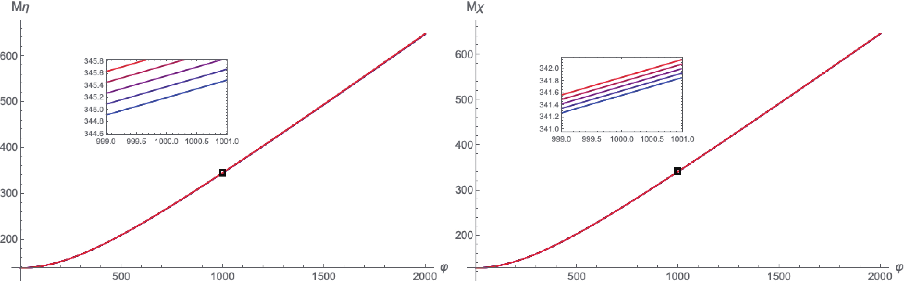
Figure 6. (color online) Figures showing how effective masses vary with φ for different Hubble parameters at initial time. Parameters are taken as
$m_{\chi} = 1$ ,$m_\phi = 50$ ,$1/\gamma = 1000$ ,$\lambda = \lambda' = h = 0.2$ ,$H = 0.001\times n/4 \,\,\,\,(n = 0,1,2,3,4)$ . The color of the curve changes from blue to red when H increases. A segment of the curves is magnified around$\varphi = 1000$ to distinguish different curves.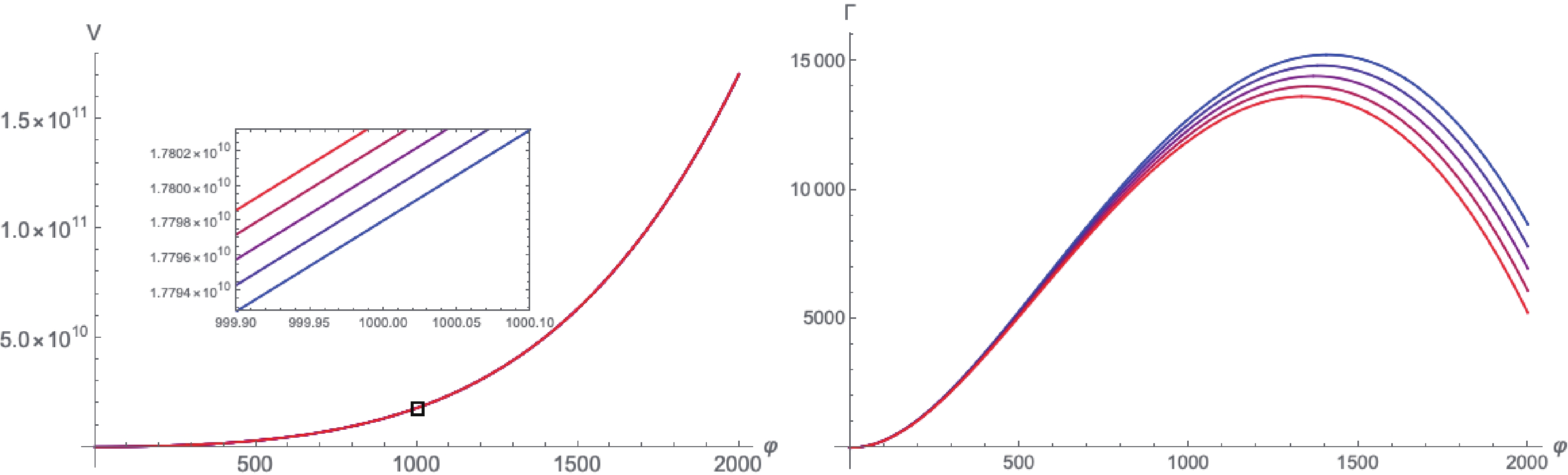
Figure 7. (color online) The figure on the left shows how the effective potential varies with φ for different Hubble parameters, and the one on the right is the plot of the dissipation coefficient. Parameters are same as in the above figures.
$ -H\left(\frac{2^{13}\pi^4\gamma^2 h^2}{\left(\lambda'^2+3h^2\right)^2}+\frac{2^{13}\pi^4\gamma^2 \lambda^2}{\left(\lambda^2+3h^2\right)^2}\right). $

(68) Because we assume pseudo-equilibrium in the evolution of the scalar field, the Hubble parameter is required to be smaller than the energy scale involved in the microscopic interactions, which is characterized by the decay rates in Eq. (34). Therefore, as an artifact of our assumptions, the coupling constants are not allowed to tend to zero, which explains the confusing fact that the dissipation coefficient in Eq. (67) seems to not vanish in the weak coupling limit. This requirement also indicates that the contributions to the dissipation coefficient from the
$ O(H^0) $ term and the term of Eq. (68) satisfies$ \begin{split}& -\left(\frac{32\pi\gamma h^2}{\lambda'^2+3h^2}+\frac{32\pi\gamma \lambda^2}{\lambda^2+3h^2}\right)\left(1+\log\frac{M_{\chi}\gamma}{2}\right)\\&\quad -H\left[\frac{2^{13}\pi^4\gamma^2 h^2}{\left(\lambda'^2+3h^2\right)^2}+\frac{2^{13}\pi^4\gamma^2 \lambda^2}{\left(\lambda^2+3h^2\right)^2}\right]\\&\quad >\left(\dfrac{32\pi\gamma}{\lambda^2+3h^2}+\dfrac{32\pi\gamma}{\lambda^2+3h^2}\right)\left(\log\dfrac{2}{M_{\chi}\gamma}-2\right), \end{split} $

(69) which is positive as the temperature is significantly greater than mass
$ M_{\chi} $ . Therefore, we conclude that although Eq. (68) is negative, the dissipation coefficient stays positive.In our calculations, we applied the assumption that the Hubble parameter H is sufficiently small, such that we can expand all terms of interest to the first order in H. The background universe is, strictly speaking, not a purely de Sitter spacetime, and the cosmic expansion is not strictly exponential. However, in such a situation, we can still obtain valuable information about the effects of cosmic expansion/contraction on the scalar field dynamics. For example, from Eq. (68), which contributes to the dissipation coefficient, we find that a de Sitter space, which is very close to a flat spacetime, has the chance of showing curved-spacetime features comparable to the flat spacetime features if the coupling constants h and
$ \lambda' $ are sufficiently small (while still ensuring that the decay rates are greater than the Hubble parameter). This is because in a de Sitter spacetime, we have to integrate over resonances due to the lack of spacetime translation invariance. Although the curved spacetime effects for the dissipation coefficient can be larger than the flat spacetime effects, which may render the dissipation coefficient negative, in this case the period for which our computations are valid would be very short, and therefore the value of ϕ would not increase indefinitely and there's no instability problem. For our computation to be valid for a sufficiently long period of time, we require that the curved spacetime effects are smaller than the flat spacetime effects so that the dissipation coefficient is positive.Our assumptions require that the temperature is significantly higher than the masses of the particles and the scale of the Hubble parameter. The effective temperature decreases as the universe expands, the corresponding approximation will fail when the temperature is of the same order as the masses. This happens only near the end of reheating; and thus the working assumptions are valid for the entire analysis if our results are to be applied to the study of reheating dynamics. We stress that our results also apply to a negative Hubble parameter H. We will be using these results to study the quantum dissipative effects in the process of matter creation in the CST bounce universe [33].
To discuss the quantum dissipative effects in the extreme conditions in the early universe, a rigorous theoretical framework of first-principle high temperature thermal quantum field theory is needed. The result we have obtained gives us a sense of the difference between the behaviour of a scalar field in a flat spacetime and in a de Sitter spacetime, which is helpful to the study of more realistic and more complicated situations, e.g., the effects of the expansion of the universe on the thermal damping rates of particles in the early universe and the production of matter within some specific inflationary or bounce models.
In this study, we only calculated the results to the first order in H. Theoretically, our approach can be extended to arbitrarily high orders, however, such attempts are not practical as the integrals become significantly more complicated. Therefore, when H becomes sufficiently large, reaching values for which the approximation we employed would fail, one needs to seek other methods to extract the interesting physics beside matter productions.
We would like to express our gratitude to Jin U Kang and Marco Drewes for useful discussions and comments on the manuscript. L.M. and H.X. thank Ella Yang for useful suggestions on improving their draft.
-
In this appendix, we calculate the free spectral function of
${\rm a} $ scalar field ξ in de Sitter spacetime with action$\tag{A1} \begin{split} S = & -\int {\rm d}^4x\sqrt{-g}\,\,\frac{1}{2}\xi\left[\frac{1}{\sqrt{-g}}\partial _\mu\left(\sqrt{-g}g^{\mu\nu}\partial _\nu\right)+m_{\xi}^{2}\right]\xi\\ =& -\int {\rm d}^4x\,\,\frac{a^3}{2}\xi\left[\left(3H\partial _t+\partial _{t}^{2}-a^{-2}\nabla^2\right)+m_{\xi}^{2}\right]\xi, \end{split} $

where
$ a = {\rm e}^{Ht} $ .If we set
$ \tau = -{\rm e}^{-Ht}/H $ ,$ \tilde{\xi} = a(t)\xi(x) $ , then the action becomes$\tag{A2} S = -\int {\rm d}\tau\int {\rm d}^3x\frac{1}{2}\tilde{\xi}\left[\partial _{\tau}^{2}-\nabla^2+\left(m_\xi^2-2H^2\right)a^2\right]\tilde{\xi}\; , $

from which we obtain the equation of motion for
$ \tilde{\xi} $ :$\tag{A3} \left[\frac{\partial ^2}{\partial \tau^2}-\nabla^2+(m_\xi^2-2H^2)a^2\right]\tilde{\xi}({{x}},\tau) = 0. $

If we expand
$ \tilde{\xi}({{x}},\tau) $ as$\tag{A4} \tilde{\xi}({{x}},\tau) = \int \frac{{\rm d}^3k}{(2\pi)^3}\tilde{\xi}({{k}},\tau){\rm e}^{{\rm i}{{k}}\cdot {{x}}}+ {\rm h.c.} $

To solve the equation of motion, we employ the Wentzel-Kramers-Brillouin (WKB) method and obtain
$\tag{A5} \tilde{\xi}({{x}},\tau) = \int \frac{{\rm d}^3k}{(2\pi)^3}\left\{ A_k \frac{\exp\left[ -{\rm i}\int_{\tau_0}^{\tau}\omega(\tau'){\rm d}\tau'\right]}{\sqrt{2\omega(\tau)}}{\rm e}^{{\rm i}{{k}}\cdot {{x}}}+{\rm h.c.}\; \right\}, $

where
$ \tau_0 $ is a constant of integration,$ A_k $ a momentum-dependent operator, and$\tag{A6} \omega(\tau) = \sqrt{{{k}}^2+(m_\xi^2-2H^2)a^2}\; . $

The conjugate momentum is given by,
$\begin{split} \tilde{\pi}({{x}},\tau) = \int \frac{{\rm d}^3k}{(2\pi)^3}\frac{1}{\sqrt{2}}\left[-\frac{1}{2}H(m_\xi^2-2H^2)a^3\omega^{-5/2}-{\rm i}\omega^{1/2}\right] \end{split}$

$\tag{A7}\begin{split} \times A_k\exp\left(-{\rm i}\int_{\tau_0}^{\tau}\omega(\tau'){\rm d}\tau'\right){\rm e}^{{\rm i}{{k}}\cdot {{x}}}+\rm h.c.\; . \end{split}$

From the commutation relation
$ \left[\tilde{\xi}({{x}},\tau),\tilde{\pi}({{x}}',\tau)\right] = i \delta^3({{x}}-{{x}}') $ , we obtain$ \left[A_{{{k}}},A_{{{k}}'}^\dagger\right] = \delta^3({{k}}-{{k}}') $ . With this commutation relation of$ A_{{{k}}} $ and$ A_{{{k}}'}^\dagger $ we can calculate the free spectral function using Eq. (74):$ \tag{A8} \begin{split}&\Delta^-({{k}},t_1,t_2) = {\rm i}\left\langle\left[\frac{\tilde{\xi}(\tau_1)}{a(t_1)},\frac{\tilde{\xi}(\tau_2)}{a(t_2)}\right]\right\rangle_\beta\\ = & \frac{1}{a(t_1)^{3/2}a(t_2)^{3/2}\sqrt{\Omega_\xi(t_1)}\sqrt{\Omega_\xi(t_2)}}\sin\left[\int_{t_2}^{t_1}\Omega_\xi(t'){\rm d}t'\right], \end{split}$

where
$\tag{A9} \Omega_\xi(t)\equiv \sqrt{{{k}}^2/a(t)^2+(m_\xi^2-2H^2)}\; . $

-
In this appendix we present the relevant formulae that we have used in computing the integrals associated with the Feynman diagrams.
-
When solving the integrals in Eq. (20), we encounter expressions of the following form,
$ \tag{B1} h_n(y) = \frac{1}{\Gamma(n)}\int_{0}^{\infty} {\rm d}x\frac{x^{n-1}}{\sqrt{x^2+y^2}}\frac{1}{{\rm e}^{\sqrt{x^2+y^2}}-1}\quad (n\in {\mathbb{Z}}^{+}). $

By expanding
$ 1/\{[\exp(\sqrt{x^2+y^2})]-1\} $ around$ \sqrt{x^2+y^2} = 0 $ into a Laurent series, integrating over x and then expanding the expression around$ y = 0 $ , we obtain$\tag{B2} \begin{split} h_1(y) =& \frac{\pi}{2y}+\frac{1}{2}\log\frac{y}{4\pi}+\frac{\gamma_E}{2}\\ & +\sum\limits_{m = 1}^{\infty}\frac{(-1)^{m}}{2^{m+1}}\frac{(2m-1)!!}{m!}\zeta(2m+1)\left(\frac{y}{2\pi}\right)^{2m}\; . \end{split} $

It is easy to verify that
$ h_n(y) $ satisfies$ \tag{B3} \frac{{\rm d}h_{n+1}}{{\rm d}y} = -\frac{yh_{n-1}}{n}\; . $

Setting
$ n = 2 $ and integrating the above equality, we have$ \begin{split} h_3(y) =& -\frac{1}{2}\int yh_1(y){\rm d}y+\frac{\pi^2}{12}\\ = & \frac{\pi^2}{12}-\frac{\pi y}{4}-\left(\frac{\gamma_E}{8}-\frac{1}{16}\right)y^2-\frac{y^2}{8}\log\frac{y}{4\pi} \end{split} $

$ \tag{B4} \begin{split} +\sum\limits_{m = 1}^{\infty}\frac{(-1)^{m+1}}{2^{m+3}}\frac{(2m-1)!!}{(m+1)!}\frac{\zeta(2m+1)}{(2\pi)^{2m}}y^{2m+2}. \end{split} $

-
In this subsection, we calculate the real and imaginary parts of the following expressions:
$\tag{B5} \begin{split} &F^\omega\left[\theta(t){\rm{Im}}\int \frac{{\rm d}^3q}{(2\pi)^3}\left(K_0+t K_1+t^2K_2\right){\rm e}^{-2{\rm i}\omega_q t-\alpha t/\omega_q}\right],\\ &F^\omega\left[\theta(t){\rm{Im}}\int \frac{{\rm d}^3q}{(2\pi)^3}\left(K_0+t K_1+t^2K_2\right){\rm e}^{-\alpha t/\omega_q}\right], \end{split} $

where
$ F^\omega $ denotes a Fourier transformation w.r.t. t and$ K_0, K_1,K_2 $ are rational functions of$ {{q}}^2 $ . We use K to denote any of$ K_0,K_1,K_2 $ and calculate the following integral:$ \tag{B6} \begin{split} & F^{\omega}\left[ \theta(t) {\rm{Im}} \int \frac{{\rm d}^{3} q}{(2 \pi)^{3}} K\left(\omega_{q}\right) {\rm e}^{-2 {\rm i} \omega_{q} t- \frac{\alpha}{\omega_q} t}\right]\\ = & \int \frac{{\rm d}^3 q}{(2\pi)^3}\left[-{\rm i}{\rm{Re}}K(\omega_q)F^\omega\left(\theta(t)\frac{{\rm e}^{-2{\rm i}\omega_q t}-{\rm e}^{2{\rm i}\omega_q t}}{2}{\rm e}^{-\frac{\alpha}{\omega_q}t}\right)\right.\\&\left.+{\rm{Im}}K(\omega_q)F^\omega\left(\theta(t)\frac{{\rm e}^{-2{\rm i}\omega_q t}+{\rm e}^{2{\rm i}\omega_q t}}{2}{\rm e}^{-\frac{\alpha}{\omega_q}t}\right)\right]. \end{split} $

Carrying out the Fourier transformation in the integrand and changing the variable of integration to
$ \omega_q = \sqrt{{{q}}^2+m^2} $ , the integral becomes$\tag{B7} \begin{split}&\frac{1}{(2 \pi)^{3}} \int_{m}^{\infty} {\rm d} \omega_{q} \frac{\omega_{q}}{\sqrt{\omega_{q}^{2}-m^{2}}} 4 \pi\left(\omega_{q}^{2}-m^{2}\right)\times \bigg\{ {\rm{Re}}K(\omega_q)\left[\frac{1}{2}\left(\dfrac{\omega-2\omega_q}{(\omega-2\omega_q)^2+(\alpha/\omega_q)^2}-\frac{\omega+2\omega_q}{(\omega+2\omega_q)^2+(\alpha/\omega_q)^2}\right)\right. \left.-{\rm i}\left(\frac{\alpha/(2\omega_q)}{(\omega-2\omega_q)^2+(\alpha/\omega_q)^2}-\frac{\alpha/(2\omega_q)}{(\omega+2\omega_q)^2+(\alpha/\omega_q)^2}\right)\right] + \\ &{\rm{Im}}K(\omega_q)\left[\frac{{\rm i}}{2}\left(\dfrac{\omega+2\omega_q}{(\omega+2\omega_q)^2+(\alpha/\omega_q)^2}+\frac{\omega-2\omega_q}{(\omega-2\omega_q)^2+(\alpha/\omega_q)^2}\right)\right. \left.+\left(\frac{\alpha/(2\omega_q)}{(\omega+2\omega_q)^2+(\alpha/\omega_q)^2}+\frac{\alpha/(2\omega_q)}{(\omega-2\omega_q)^2+(\alpha/(2\omega_q))^2}\right)\right]\bigg\}. \\[-20pt] \end{split} $

Because we only calculate to the lowest order in α, the above expression can be further simplified to
$\tag{B8} \begin{split}&\frac{1}{(2 \pi)^{3}} \int_{m}^{\infty} {\rm d} \omega_{q} \frac{\omega_{q}}{\sqrt{\omega_{q}^{2}-m^{2}}} 4 \pi\left(\omega_{q}^{2}-m^{2}\right)\times\left\{{\rm{Re}}K(\omega_q)\left[\frac{2\omega_q}{\omega^2-4\omega_q^2}-{\rm i}\left(\frac{\alpha}{2\omega_q(\omega-2\omega_q)^2}-\frac{\alpha}{2\omega_q(\omega+2\omega_q)^2}\right)\right]\right.\\ &\left.+{\rm{Im}}K(\omega_q)\left[{\rm i}\frac{\omega}{\omega^2-4\omega_q^2}+\left(\frac{\alpha}{2\omega_q(\omega-2\omega_q)^2}+\frac{\alpha}{2\omega_q(\omega+2\omega_q)^2}\right)\right]\right\} \equiv I_{\rm re}\left[K(\omega_q)\right]+{\rm i}I_{\rm im}\left[K(\omega_q)\right], \end{split} $

where
$\tag{B9} \left\{ \begin{split}& I_{\rm r e}\left[K\left(\omega_{{q}}\right)\right] = \frac{1}{(2 \pi)^{3}} \int_{m}^{\infty} {\rm d} \omega_{{q}} 4 \pi \omega_{{q}} \sqrt{\omega_{{q}}^{2}-m^2}\Bigg\{{\rm{Re}} K\left(\omega_{{q}}\right) \frac{2 \omega_{{q}}}{\omega^{2}-4 \omega_{{q}}^{2}} +{\rm{Im}} K\left(\omega_{{q}}\right)\left[\frac{\alpha}{2\omega_{{q}}\left(\omega+2 \omega_{{q}}\right)^{2}}+\frac{\alpha}{2\omega_{{q}}\left(\omega-2 \omega_{{q}}\right)^{2}}\right]\Bigg\}\\ & I_{\rm im}\left[K\left(\omega_{{q}}\right)\right] = \frac{1}{(2 \pi)^{3}} \int_{m}^{\infty} {\rm d} \omega_{{q}} 4 \pi \omega_{{q}} \sqrt{\omega_{{q}}^{2}-m^2}\Bigg\{{\rm{Im}} K\left(\omega_{{q}}\right) \frac{\omega}{\omega^{2}-4 \omega_{{q}}^{2}}-{\rm{Re}} K\left(\omega_{{q}}\right)\left[\frac{\alpha}{2\omega_{{q}}\left(\omega-2 \omega_{{q}}\right)^{2}}-\frac{\alpha}{2\omega_{{q}}\left(\omega+2 \omega_{{q}}\right)^{2}}\right]\Bigg\} \end{split} \right.\; . $

We arrive at
$ \tag{B10} \begin{split}& {\rm{Im}} F^{\omega}\left[\theta(t) {\rm{Im}} \int \frac{{\rm d}^{3} q}{(2 \pi)^{3}}\left(K_{0}+t K_{1}+t^{2} K_{2}\right) {\rm e}^{-2 {\rm i} \omega_{q} t- \frac{\alpha}{\omega_{q}} t}\right] = {\rm{Im}} F^{\omega} \left[\theta(t) {\rm{Im}} \int \frac{{\rm d}^{3} q}{(2 \pi)^{3}}K_{0} {\rm e}^{-2 {\rm i} \omega_{q} t- \frac{\alpha}{\omega_{q}} t}\right]+{\rm{Im}}\Bigg\{\left(-{\rm i} \frac{\partial}{\partial \omega}\right) F^{\omega} \left[\theta(t) {\rm{Im}} \int \frac{{\rm d}^{3} q}{(2 \pi)^{3}}K_{1}{\rm e}^{-2 {\rm i} \omega_{q} t-\frac{\alpha}{\omega_{q}}t} \right]\Bigg\}\\ & +{\rm{Im}}\Bigg\{\left(-\frac{\partial^{2}}{\partial \omega^{2}}\right) F^{\omega} \left[\theta(t) {\rm{Im}} \int \frac{{\rm d}^{3} q}{(2 \pi)^{3}}K_{3}{\rm e}^{-2 {\rm i} \omega_{q} t-\frac{\alpha}{\omega_{q}} t}\right]\Bigg\} = I_{\rm i m}\left[K_{0}\right]-\frac{\partial}{\partial \omega} I_{\rm r e}\left[K_{1}\right]-\frac{\partial^{2}}{\partial \omega^{2}} I_{\rm i m}\left[K_{2}\right]\; . \end{split} $

In a similar way, we obtain
$ \tag{B11} {\rm{Re}} F^{\omega}\left[\theta(t) {\rm{Im}} \int \frac{{\rm d}^{3} q}{(2 \pi)^{3}}\left(K_{0}+t K_{1}+t^{2} K_{2}\right) {\rm e}^{-2 {\rm i} \omega_{q} t- \frac{\alpha}{\omega_{q}} t}\right] = I_{\rm re}\left[K_{0}\right]+\frac{\partial}{\partial \omega} I_{\rm im}\left[K_{1}\right]-\frac{\partial^{2}}{\partial \omega^{2}} I_{\rm re}\left[K_{2}\right]\; , $

$ \tag{B12} \begin{split} F^{\omega}\left[\theta(t) {\rm{Im}} \int \frac{{\rm d}^{3} q}{(2 \pi)^{3}}\left(K_{0}+t K_{1}+t^{2} K_{2}\right) {\rm e}^{- \frac{\alpha}{\omega_{q}} t}\right] =& \int \frac{{\rm d}^3q}{(2\pi)^3}\left({\rm{Im}}K_0\frac{\omega_q \alpha}{\alpha^2+\omega^2\omega^2_q}+{\rm{Im}}K_1\frac{\partial}{\partial \omega}\frac{\omega\omega^2_q}{\alpha^2+\omega^2\omega^2_q}-{\rm{Im}}K_2\frac{\partial^2}{\partial \omega^2}\frac{\omega_q \alpha}{\alpha^2+\omega^2\omega^2_q}\right)\\ & +{\rm i}\int \frac{{\rm d}^3q}{(2\pi)^3}\left({\rm{Im}}K_0\frac{\omega\omega^2_q}{\alpha^2+\omega^2\omega^2_q}-{\rm{Im}}K_1\frac{\partial }{\partial \omega}\frac{\omega_q\alpha}{\alpha^2+\omega^2\omega^2_q}-{\rm{Im}}K_2\frac{\partial ^2}{\partial \omega^2}\frac{\omega\omega^2_q}{\alpha^2+\omega^2\omega^2_q}\right)\; . \end{split} $

-
In this appendix, we present the detailed calculation of the the tadpole diagram. Inserting the propagator Eq. (8) into Eq. (20),
${\rm{we}} $ have$\tag{C1} \begin{split} \Pi^R(t_1,t_2) =& \frac{1}{2}\delta(t_1-t_2)\sum\limits_{\xi = \eta,\chi}\int \frac{{\rm d}^3p}{(2\pi)^3}\frac{g_\xi}{a(t_1)^3\sqrt{{{p}}^2/a(t_1)^2+M^2_\xi}}\left[\frac{1}{2}+\frac{1}{{\rm e}^{\sqrt{{{p}}^2\beta(t_1)^2/a(t_1)^2+M^2_\xi\beta(t_1)^2}}-1}\right]\\ = & \delta(t_1-t_2)\frac{1}{4\pi^2\beta(t_1)^2}\sum\limits_{\xi = \eta,\chi}\int {\rm d}x\,g_\xi\left[\frac{1}{2}\frac{x^2}{\sqrt{x^2+M^2_\xi\beta(t_1)^2}}+\frac{x^2}{\sqrt{x^2+M^2_\xi\beta(t_1)^2}}\frac{1}{{\rm e}^{\sqrt{x^2+M_\xi^2\beta(t_1)^2}}-1}\right]\; . \end{split} $

We replace the divergent integrals that are independent of time by the constants
$ C_1 $ and$ C_2 $ :$\tag{C2} \begin{split} C_1 =& \frac{1}{2}\sum\limits_{\xi = \eta,\chi}\int \frac{{\rm d}^3p}{(2\pi)^3}\frac{g_\xi}{2\sqrt{{{p}}^2+M_\xi^2}}+{\rm{counter}}\;{\rm{terms}},\\ C_2 = &\frac{1}{2}\sum\limits_{\xi = \eta,\chi}\int\frac{{\rm d}^3p}{(2\pi)^3}\left[\frac{g_\xi}{\sqrt{{{p}}^2+M_\xi^2}}+\frac{g_\xi M_\xi^2}{2({{p}}^2+M_\xi^2)^{3/2}}\right]\\ & +{\rm{counter terms}}. \end{split} $

yielding
$ \Pi^R(t_1,t_2) $ in the following form,$ \tag{C3} \begin{split}&\Pi^R(t_1,t_2) = \delta(t_1-t_2)\\&\times\left\{C_1-C_2Ht_1+\frac{1}{2\pi^2\beta(t_1)^2}\sum\limits_{\xi = \eta,\chi}g_\xi h_3\left[M_\xi\beta(t_1)\right]\right\}\; . \end{split} $

Comparing with the case of
$ H = 0 $ ,$\tag{C4} \Pi^R(t_1,t_2)\approx\delta(t_1\!-\!t_2)\left[C_1\!\!+\!\! \sum\limits_{\xi = \eta,\chi}\int\frac{{\rm d}^3p}{(2\pi)^3}\frac{g_\xi}{2\sqrt{{{p}}^2+M_\xi^2}}\cdot\frac{1}{\exp\left(\dfrac{\beta_0\sqrt{{{p}}^2+M_\xi^2}}{a_0}\right)\!-\!1}\right], $

we can conclude that
$ C_1 = 0 $ at zero temperature in flat spacetime. Furthermore, the propagator of ϕ has a pole at the physical mass: the first term and the second term in the$ C_2 $ integral are proportional to$ C_1 $ or to the derivative of$ C_1 $ with respect to$ M_\xi $ , we deduce that$ C_2 = 0 $ . The renormalized$ \Pi^R(t_1,t_2) $ is finally given by$\tag{C5} \Pi^R(t_1,t_2) = \delta(t_1-t_2)\left\{\frac{1}{2\pi^2\beta(t_1)^2}\sum\limits_{\xi = \eta,\chi}g_\xi h_3\left[M_\xi\beta(t_1)\right]\right\}\; . $

-
Let us now turn to the contribution of the sunset diagram to the self-energy,
$\tag{D1} \begin{split} -{\rm i}\left[\Pi^R(t_1,t_2)\right]_{\rm{sunset}} = -{\rm i}h^2\theta(t_1-t_2)\int \frac{{\rm d}^3k}{(2\pi)^3}\frac{{\rm d}^3l}{(2\pi)^3}{\rm{Im}}\left[(\Delta_{\chi})_>({{k}},t_1,t_2)\right. \left.\times(\Delta_{\chi})_>({{l}},t_1,t_2)(\Delta_{\eta})_>({{k}}+{{l}},t_1,t_2)\right]\; . \end{split} $

By expanding the propagators to the first order in H and inserting them into the above equation, we obtain the following expression of the imaginary part
${\rm{of}} $ κ,$ \tag{D2} \begin{split}& {\rm{Im}}\kappa(t_1,\omega) = \frac{h^2}{8} {\rm{Im}}F^\omega\Bigg\{\theta(t)\int \frac{{\rm d}^{3}k}{(2\pi)^3}\frac{{\rm d}^3l}{(2\pi)^3} {\rm{Im}}\frac { 1 } { \omega _ { \eta q } \omega_{\chi k} \omega_{\chi l} }\left[\left( 1 - 9 H t _ { 1 } + \frac { 9 } { 2 } H t \right) +\left( H t _ { 1 } - \frac { 1 } { 2 } H t \right) \left(3 - \frac { M_{\eta} ^ { 2 } } { \omega _ { \eta q } ^ { 2 } } - \frac { M_{\chi} ^ { 2 } } { \omega_{\chi k} ^ { 2 } } - \frac { M_{\chi}^ { 2 } } { \omega_{\chi l} ^ { 2 } } \right)\right.\\& \left. - H \left( t _ { 1 } - t \right) \left( f (\omega_{\eta q}) \frac { \gamma M_{\eta} ^ { 2 } } { \omega _ { \eta q } } + f (\omega_{\chi k}) \frac { \gamma M_{\chi}^ { 2 } } { \omega_{\chi k} } + f (\omega_{\chi l}) \frac { \gamma M_{\chi} ^ { 2 } } { \omega_{\chi l} } \right) + {\rm i} H \left( 2 t _ { 1 } t - t ^ { 2 } \right) \left( \frac { \boldsymbol { q } ^ { 2 } } { 2 \omega _ { \eta q } } + \frac { \boldsymbol { k } ^ { 2 } } { 2 \omega_{\chi k} } + \frac { \boldsymbol { l } ^ { 2 } } { 2 \omega_{\chi l} } \right)\right]\\ &\times \left( 1 + f (\omega_{\eta q})\right) \left( 1 + f (\omega_{\chi k}) \right) \left( 1 + f (\omega_{\chi l}) \right) \exp \left[ - {\rm i} \left( \omega _ { \eta q } + \omega_{\chi k} + \omega_{\chi l} \right) t-\Gamma_{\chi}(\omega_{\chi k})t/2-\Gamma_{\chi}(\omega_{\chi l})t/2 \right]\Bigg\} \\ & + \left( \omega _ { \eta q } \rightarrow - \omega _ { \eta q } , \omega_{\chi k} \rightarrow - \omega_{\chi k} , \omega_{\chi l} \rightarrow - \omega_{\chi l} \right) + \left( \omega _ { \eta q } \rightarrow - \omega _ { \eta q } , \omega_{\chi k} \rightarrow - \omega_{\chi k} , \omega_{\chi l} \rightarrow \omega_{\chi l} \right) + \left( \omega _ { \eta q } \rightarrow \omega _ { \eta q } , \omega_{\chi k} \rightarrow \omega_{\chi k} , \omega_{\chi l} \rightarrow - \omega_{\chi l} \right)\\ & + \left( \omega _ { \eta q } \rightarrow - \omega _ { \eta q } , \omega_{\chi k} \rightarrow \omega_{\chi k} , \omega_{\chi l} \rightarrow - \omega_{\chi l} \right) + \left( \omega _ { \eta q } \rightarrow \omega _ { \eta q } , \omega_{\chi k} \rightarrow - \omega_{\chi k} , \omega_{\chi l} \rightarrow \omega_{\chi l} \right)\\ & + \left( \omega _ { \eta q } \rightarrow \omega _ { \eta q } , \omega_{\chi k} \rightarrow - \omega_{\chi k} , \omega_{\chi l} \rightarrow - \omega_{\chi l} \right) + \left( \omega _ { \eta q } \rightarrow - \omega _ { \eta q } , \omega_{\chi k} \rightarrow \omega_{\chi k} , \omega_{\chi l} \rightarrow \omega_{\chi l} \right)\\ =& \frac{h^2}{8} {\rm{Im}}F^\omega\Bigg\{\theta(t)\int \frac{{\rm d}^{3}k}{(2\pi)^3}\frac{{\rm d}^3l}{(2\pi)^3}\frac { 1 } { \omega _ { \eta q } \omega_{\chi k} \omega_{\chi l} }\Bigg\{-\sin \left[ \left( \omega _ { \eta q } + \omega_{\chi k} + \omega_{\chi l} \right) t \right]\exp \left(-\Gamma_{\chi}(\omega_{\chi k})t/2-\Gamma_{\chi}(\omega_{\chi l})t/2\right) \\ & \times\left[ \left( 1 - 9 H t _ { 1 } \right) \gamma _ { 0 } \left( \omega _ { \eta q } , \omega_{\chi k} , \omega_{\chi l} \right) + H t _ { 1 } \gamma _ { 1 } \left( \omega _ { \eta q } , \omega_{\chi k} , \omega_{\chi l} \right) - H t _ { 1 } \gamma _ { 2 } \left( \omega _ { \eta q } , \omega_{\chi k} , \omega_{\chi l} \right) \right] \\ & +t \cos \left[ \left( \omega _ { \eta q } + \omega_{\chi k} + \omega_{\chi l} \right) t \right]\exp \left(-\Gamma_{\chi}(\omega_{\chi k})t/2-\Gamma_{\chi}(\omega_{\chi l})t/2\right)\cdot2 H t _ { 1 } \gamma _ { 3 } \left( \omega _ { \eta q } , \omega_{\chi k} , \omega_{\chi l} \right) \\ & -t \sin \left[ \left( \omega _ { \eta q } + \omega_{\chi k} + \omega_{\chi l} \right) t \right]\exp \left(-\Gamma_{\chi}(\omega_{\chi k})t/2-\Gamma_{\chi}(\omega_{\chi l})t/2\right)\\ & \times \Bigg[ \frac { 9 } { 2 } H \gamma _ { 0 } \left( \omega _ { \eta q } , \omega_{\chi k} , \omega_{\chi l} \right)- \frac { 1 } { 2 } H \gamma _ { 1 } \left( \omega _ { \eta q } , \omega_{\chi k} , \omega_{\chi l} \right) + H \gamma _ { 2 } \left( \omega _ { \eta q } , \omega_{\chi k} , \omega_{\chi l} \right) \Bigg] \\ & - t ^ { 2 } \cos \left[ \left( \omega _ { \eta q } + \omega_{\chi k} + \omega_{\chi l} \right) t \right]\exp \left(-\Gamma_{\chi}(\omega_{\chi k})t/2-\Gamma_{\chi}(\omega_{\chi l})t/2\right) \cdot H \gamma _ { 3 } \left( \omega _ { \eta q } , \omega_{\chi k} , \omega_{\chi l} \right)\Bigg\}\\ & \times \left( 1 + f (\omega_{\eta q}) \right) \left( 1 + f(\omega_{\chi k}) \right) \left( 1 + f(\omega_{\chi l}) \right)\Bigg\} + \left( \omega _ { \eta q } \rightarrow - \omega _ { \eta q } , \omega_{\chi k} \rightarrow - \omega_{\chi k} , \omega_{\chi l} \rightarrow - \omega_{\chi l} \right)\\ & + \left( \omega _ { \eta q } \rightarrow - \omega _ { \eta q } , \omega_{\chi k} \rightarrow - \omega_{\chi k} , \omega_{\chi l} \rightarrow \omega_{\chi l} \right) + \left( \omega _ { \eta q } \rightarrow \omega _ { \eta q } , \omega_{\chi k} \rightarrow \omega_{\chi k} , \omega_{\chi l} \rightarrow - \omega_{\chi l} \right)\\ & + \left( \omega _ { \eta q } \rightarrow - \omega _ { \eta q } , \omega_{\chi k} \rightarrow \omega_{\chi k} , \omega_{\chi l} \rightarrow - \omega_{\chi l} \right) + \left( \omega _ { \eta q } \rightarrow \omega _ { \eta q } , \omega_{\chi k} \rightarrow - \omega_{\chi k} , \omega_{\chi l} \rightarrow \omega_{\chi l} \right)\\ & + \left( \omega _ { \eta q } \rightarrow \omega _ { \eta q } , \omega_{\chi k} \rightarrow - \omega_{\chi k} , \omega_{\chi l} \rightarrow - \omega_{\chi l} \right) + \left( \omega _ { \eta q } \rightarrow - \omega _ { \eta q } , \omega_{\chi k} \rightarrow \omega_{\chi k} , \omega_{\chi l} \rightarrow \omega_{\chi l} \right), \end{split}$

where
$ \Gamma_{\chi}(\omega_{\chi k})\approx\frac{\lambda'^2+3h^2}{256\pi^3\gamma^2\omega_{\chi k}}, \Gamma_{\chi}(\omega_{\chi l})\approx\frac{\lambda'^2+3h^2}{256\pi^3\gamma^2\omega_{\chi l}} $ and$ \tag{D3}\left\{ \begin{split} & \gamma _ { 0 } \left( \omega _ { \eta q } , \omega_{\chi k} , \omega_{\chi l} \right) = 1\; ,\\ & \gamma _ { 1 } \left( \omega _ { \eta q } , \omega_{\chi k} , \omega_{\chi l} \right) = 3 - \frac { M_{\eta} ^ { 2 } } { \omega _ { \eta q } ^ { 2 } } - \frac { M_{\chi} ^ { 2 } } { \omega_{\chi k} ^ { 2 } } - \frac { M_{\chi}^ { 2 } } { \omega_{\chi l} ^ { 2 } }\; ,\\ & \gamma _ { 2 } \left( \omega _ { \eta q } , \omega_{\chi k} , \omega_{\chi l} \right) = f (\omega_{\eta q}) \frac { \gamma M_{\eta} ^ { 2 } } { \omega _ { \eta q } } + f (\omega_{\chi k}) \frac { \gamma M_{\chi}^ { 2 } } { \omega_{\chi k} } + f (\omega_{\chi l})\frac { \gamma M_{\chi} ^ { 2 } } { \omega_{\chi l} }\; ,\\ & \gamma _ { 3 } \left( \omega _ { \eta q } , \omega_{\chi k} , \omega_{\chi l} \right) = \frac { \boldsymbol { q } ^ { 2 } } { 2 \omega _ { \eta q } } + \frac { \boldsymbol { k } ^ { 2 } } { 2 \omega_{\chi k} } + \frac { \boldsymbol { l } ^ { 2 } } { 2 \omega_{\chi l} } \; . \end{split} \right.$

We note that in Eq. (97), there are four kinds of Fourier transformations, which involve
$ \sin(\omega_{\eta q}+\omega_{\chi k}+\omega_{\chi l}), $ $ t\cos(\omega_{\eta q}+\omega_{\chi k}+\omega_{\chi l}) , $ $ t\sin(\omega_{\eta q}+\omega_{\chi k}+\omega_{\chi l}) , $ and$ t^2\cos(\omega_{\eta q}+\omega_{\chi k}+\omega_{\chi l}) , $ respectively. For the first two, we carry out the Fourier transformations and perform the angle integrals, expressing them in the following form:$\tag{D4} \begin{split} I_s[\gamma_i] \equiv & -{\rm{Im}}F^\omega\Bigg\{\theta(t)\int \frac{{\rm d}^{3}k}{(2\pi)^3}\frac{{\rm d}^3l}{(2\pi)^3} \sin \left[ \left( \omega _ { \eta q } + \omega_{\chi k} + \omega_{\chi l} \right) t \right]\exp \left(-\Gamma_{\chi}(\omega_{\chi k})t/2-\Gamma_{\chi}(\omega_{\chi l})t/2\right) \frac { \gamma_i(\omega_{\eta q},\omega_{\chi k},\omega_{\chi l}) } { \omega _ { \eta q } \omega_{\chi k} \omega_{\chi l} } \left( 1 + f (\omega_{\eta q}) \right) \left( 1 + f(\omega_{\chi k}) \right) \left( 1 + f(\omega_{\chi l}) \right)\Bigg\}\\ & + \left( \omega _ { \eta q } \rightarrow - \omega _ { \eta q } , \omega_{\chi k} \rightarrow - \omega_{\chi k} , \omega_{\chi l} \rightarrow - \omega_{\chi l} \right) + \left( \omega _ { \eta q } \rightarrow - \omega _ { \eta q } , \omega_{\chi k} \rightarrow - \omega_{\chi k} , \omega_{\chi l} \rightarrow \omega_{\chi l} \right) + \left( \omega _ { \eta q } \rightarrow \omega _ { \eta q } , \omega_{\chi k} \rightarrow \omega_{\chi k} , \omega_{\chi l} \rightarrow - \omega_{\chi l} \right)\\ &+ \left( \omega _ { \eta q } \rightarrow - \omega _ { \eta q } , \omega_{\chi k} \rightarrow \omega_{\chi k} , \omega_{\chi l} \rightarrow - \omega_{\chi l} \right) + \left( \omega _ { \eta q } \rightarrow \omega _ { \eta q } , \omega_{\chi k} \rightarrow - \omega_{\chi k} , \omega_{\chi l} \rightarrow \omega_{\chi l} \right)\\& + \left( \omega _ { \eta q } \rightarrow \omega _ { \eta q } , \omega_{\chi k} \rightarrow - \omega_{\chi k} , \omega_{\chi l} \rightarrow - \omega_{\chi l} \right) + \left( \omega _ { \eta q } \rightarrow - \omega _ { \eta q } , \omega_{\chi k} \rightarrow \omega_{\chi k} , \omega_{\chi l} \rightarrow \omega_{\chi l} \right)\\ \approx & \frac { 1 } { 4 ( 2 \pi ) ^ { 3 } } \int _ { M_{\chi} } ^ { \infty } {\rm d} \omega_{\chi l} \int _ { M_{\chi} t _ { 1 } - } ^ { M_{\chi} t _ { 1 + } } {\rm d} \omega_{\chi k}\big[\gamma _ { i } \left( - \omega + \omega_{\chi k} + \omega_{\chi l} , - \omega_{\chi k} , - \omega_{\chi l} \right) \left( 1 + f \left( \omega_{\chi k} + \omega_{\chi l} - \omega \right) \right) f \left( \omega_{\chi k} \right) f \left( \omega_{\chi l} \right)\\ & - \gamma _ { i } \left( \omega - \omega_{\chi k} - \omega_{\chi l} , \omega_{\chi k} , \omega_{\chi l} \right) f \left( \omega_{\chi k} + \omega_{\chi l} - \omega \right) \left( 1 + f \left( \omega_{\chi k} \right) \right) \left( 1 + f \left( \omega_{\chi l} \right) \right)\big]-\left(\omega\to -\omega\right)\; , \end{split} $

$\tag{D5} \begin{split} -\frac{\partial}{\partial\omega}I_c[\gamma_i] \equiv & {\rm{Im}}F^\omega\Bigg\{\theta(t)\int \frac{{\rm d}^{3}k}{(2\pi)^3}\frac{{\rm d}^3l}{(2\pi)^3} t\cos \left[ \left( \omega _ { \eta q } + \omega_{\chi k} + \omega_{\chi l} \right) t \right]\exp \left(-\Gamma_{\chi}(\omega_{\chi k})t/2-\Gamma_{\chi}(\omega_{\chi l})t/2\right)\frac { \gamma_i(\omega_{\eta q},\omega_{\chi k},\omega_{\chi l}) } { \omega _ { \eta q } \omega_{\chi k} \omega_{\chi l} } \left( 1 + f (\omega_{\eta q}) \right) \left( 1 + f (\omega_{\chi k})\right) \left( 1 + f (\omega_{\chi l})\right)\Bigg\} \\ & + \left( \omega _ { \eta q } \rightarrow - \omega _ { \eta q } , \omega_{\chi k} \rightarrow - \omega_{\chi k} , \omega_{\chi l} \rightarrow - \omega_{\chi l} \right) + \left( \omega _ { \eta q } \rightarrow - \omega _ { \eta q } , \omega_{\chi k} \rightarrow - \omega_{\chi k} , \omega_{\chi l} \rightarrow \omega_{\chi l} \right) + \left( \omega _ { \eta q } \rightarrow \omega _ { \eta q } , \omega_{\chi k} \rightarrow \omega_{\chi k} , \omega_{\chi l} \rightarrow - \omega_{\chi l} \right)\\ & + \left( \omega _ { \eta q } \rightarrow - \omega _ { \eta q } , \omega_{\chi k} \rightarrow \omega_{\chi k} , \omega_{\chi l} \rightarrow - \omega_{\chi l} \right) + \left( \omega _ { \eta q } \rightarrow \omega _ { \eta q } , \omega_{\chi k} \rightarrow - \omega_{\chi k} , \omega_{\chi l} \rightarrow \omega_{\chi l} \right)\\ & + \left( \omega _ { \eta q } \rightarrow \omega _ { \eta q } , \omega_{\chi k} \rightarrow - \omega_{\chi k} , \omega_{\chi l} \rightarrow - \omega_{\chi l} \right) + \left( \omega _ { \eta q } \rightarrow - \omega _ { \eta q } , \omega_{\chi k} \rightarrow \omega_{\chi k} , \omega_{\chi l} \rightarrow \omega_{\chi l} \right)\\ \approx & -\frac{\partial}{\partial \omega}\Bigg\{\frac { 1 } { 4 ( 2 \pi ) ^ { 3 } } \int _ { M_{\chi} } ^ { \infty } {\rm d} \omega_{\chi l} \int _ { M_{\chi} t _ { 1 } - } ^ { M_{\chi} t _ { 1 + } } {\rm d} \omega_{\chi k}\big[\gamma _ { i } \left( - \omega + \omega_{\chi k} + \omega_{\chi l} , - \omega_{\chi k} , - \omega_{\chi l} \right) \left( 1 + f \left( \omega_{\chi k} + \omega_{\chi l} - \omega \right) \right) f \left( \omega_{\chi k} \right) f \left( \omega_{\chi l} \right)\\ & - \gamma _ { i } \left( \omega - \omega_{\chi k} - \omega_{\chi l} , \omega_{\chi k} , \omega_{\chi l} \right) f \left( \omega_{\chi k} + \omega_{\chi l} - \omega \right) \left( 1 + f \left( \omega_{\chi k} \right) \right) \left( 1 + f \left( \omega_{\chi l} \right) \right)\big]+\left(\omega\to -\omega\right)\Bigg\}, \\[-15pt] \end{split} $

where
$\tag{D6} \left\{ \begin{split} & t _ { 1 \pm } = ( u - 1 ) s \pm \sqrt { u ( u - 2 ) \left( s ^ { 2 } - 1 \right) } + \frac { \omega } { M_{\chi} } \left[ 1 - u + ( 2 u - 1 ) s ^ { 2 } \pm s \sqrt { u ( u - 2 ) \left( s ^ { 2 } - 1 \right) \left( \frac { 2 u - 3 } { u - 2 } \right) } \right]\\ & u = \frac { M_{\eta} ^ { 2 } } { 2 M_{\chi}^ { 2 } } , s = \frac { \omega_{\chi l} } {M_{\chi}} \end{split} \right.\; . $

We presently compute the derivatives of
$ I_s $ and$ I_c $ , and set$ \omega = 0 $ :$ \tag{D7} \begin{split} \left. \frac { \partial } { \partial \omega } I _ { s } \left[ \gamma _ { i } \right] \right|_ { \omega = 0 } =& 2 \cdot \frac { 1 } { 4 ( 2 \pi ) ^ { 3 } } \int _ {M_{\chi}} ^ { \infty } {\rm d} \omega_{\chi l}\int_{M_{\chi} \left[ ( u - 1 ) s - \sqrt { u ( u - 2 ) \left( s ^ { 2 } - 1 \right) } \right]}^{M_{\chi} \left[ ( u - 1 ) s + \sqrt { u ( u - 2 ) \left( s ^ { 2 } - 1 \right) } \right]} {\rm d} \omega_{\chi k} \frac { \partial } { \partial \omega } \bigg[\gamma _ { i } \left( - \omega + \omega_{\chi k} + \omega_{\chi l} , - \omega_{\chi k} , - \omega_{\chi l} \right) \left( 1 + f \left( \omega_{\chi k} + \omega_{\chi l} - \omega \right) \right) f \left( \omega_{\chi k} \right) f \left( \omega_{\chi l} \right)\\ & - \gamma _ { i } \left( \omega - \omega_{\chi k} - \omega_{\chi l} , \omega_{\chi k} , \omega_{\chi l} \right) f \left( \omega_{\chi k} + \omega_{\chi l} - \omega \right) \left( 1 + f \left( \omega_{\chi k} \right) \right) \left( 1 + f \left( \omega_{\chi l} \right) \right)\bigg]_{\omega = 0}\\ & + 2 \cdot \frac { 1 } { 4 ( 2 \pi ) ^ { 3 } } \int _ {M_{\chi}} ^ { \infty } {\rm d} \omega_{\chi l}\bigg\{M_{\chi} t_{1p}\Big[\gamma _ { i } \left( \omega_{\chi k} + \omega_{\chi l} , - \omega_{\chi k} , - \omega_{\chi l} \right) \left( 1 + f \left( \omega_{\chi k} + \omega_{\chi l} \right) \right) f \left( \omega_{\chi k} \right) f \left( \omega_{\chi l} \right)\\ & - \gamma _ { i } \left( - \omega_{\chi k} - \omega_{\chi l} , \omega_{\chi k} , \omega_{\chi l} \right) f \left( \omega_{\chi k} + \omega_{\chi l} \right) \left( 1 + f \left( \omega_{\chi k} \right) \right) \left( 1 + f \left( \omega_{\chi l} \right) \right)\Big]_{\omega_{\chi k} = M_{\chi} t_{0p}}\\ & - M_{\chi} t _ { 1 m }\Big[\gamma _ { i } \left( \omega_{\chi k} + \omega_{\chi l} , - \omega_{\chi k} , - \omega_{\chi l} \right) \left( 1 + f \left( \omega_{\chi k} + \omega_{\chi l} \right) \right) f \left( \omega_{\chi k} \right) f \left( \omega_{\chi l} \right)\\ & - \gamma _ { i } \left( - \omega_{\chi k} - \omega_{\chi l} , \omega_{\chi k} , \omega_{\chi l} \right) f \left( \omega_{\chi k} + \omega_{\chi l} \right) \left( 1 + f \left( \omega_{\chi k} \right) \right) \left( 1 + f \left( \omega_{\chi l} \right) \right)\Big]_{\omega_{\chi k} = M_{\chi} t_{0m}}\bigg\}\; , \end{split} $

$\tag{D8} \begin{split} - \left. \frac { \partial ^ { 2 } } { \partial \omega ^ { 2 } } I _ { c } \left[ \gamma _ { i } \right] \right|_ { \omega = 0 } =& - \frac { 1 } { 2 ( 2 \pi ) ^ { 3 } } \int _ { M_{\chi} } ^ { \infty } {\rm d} \omega_{\chi l}\Bigg\{\int _ { M_{\chi} t _ { 0 m } } ^ { M_{\chi} t _ { 0 p } } {\rm d} \omega_{\chi k} \frac { \partial ^ { 2 } } { \partial \omega ^ { 2 } }\Big[\gamma _ { i } \left( - \omega + \omega_{\chi k} + \omega_{\chi l} , - \omega_{\chi k} , - \omega_{\chi l} \right) \left( 1 + f \left( \omega_{\chi k} + \omega_{\chi l} - \omega \right) \right) f \left( \omega_{\chi k} \right) f \left( \omega_{\chi l} \right)\\ & - \gamma _ { i } \left( \omega - \omega_{\chi k} - \omega_{\chi l} , \omega_{\chi k} , \omega_{\chi l} \right) f \left( \omega_{\chi k} + \omega_{\chi l} - \omega \right) \left( 1 + f \left( \omega_{\chi k} \right) \right) \left( 1 + f \left( \omega_{\chi l} \right) \right)\Big]\bigg|_{\omega = 0}\\ & +M_{\chi}^2(t_{1p})^2\frac{\partial}{\partial \omega_{\chi k}}\Big[\gamma_i(\omega_{\chi k}+\omega_{\chi l},-\omega_{\chi k},-\omega_{\chi l})\left(1+f\left(\omega_{\chi k}+\omega_{\chi l}\right)\right)f\left(\omega_{\chi k}\right)f\left(\omega_{\chi l}\right)\\ & -\gamma_i\left(-\omega_{\chi k}-\omega_{\chi l},\omega_{\chi k},\omega_{\chi l}\right)f\left(\omega_{\chi k}+\omega_{\chi l}\right)\left(1+f\left(\omega_{\chi k}\right)\right)\left(1+f\left(\omega_{\chi l}\right)\right)\Big]\bigg|_{\omega_{\chi k}\to M_{\chi} t_{0p}}\\ & -M_{\chi}^2(t_{1m})^2\frac{\partial}{\partial \omega_{\chi k}}\Big[\gamma_i(\omega_{\chi k}+\omega_{\chi l},-\omega_{\chi k},-\omega_{\chi l})\left(1+f\left(\omega_{\chi k}+\omega_{\chi l}\right)\right)f\left(\omega_{\chi k}\right)f\left(\omega_{\chi l}\right)\\ & -\gamma_i\left(-\omega_{\chi k}-\omega_{\chi l},\omega_{\chi k},\omega_{\chi l}\right)f\left(\omega_{\chi k}+\omega_{\chi l}\right)\left(1+f\left(\omega_{\chi k}\right)\right)\left(1+f\left(\omega_{\chi l}\right)\right)\Big]\bigg|_{\omega_{\chi k}\to M_{\chi} t_{0m}}\Bigg\}, \end{split} $

where
$\tag{D9} \left\{ \begin{split}& u = \frac{M_{\eta}^2}{2M_{\chi}^2},\ s = \frac{\omega_{\chi l}}{M_{\chi}} ,\\ & t _ { 0 p } = ( u - 1 ) s + \sqrt { u ( u - 2 ) \left( s ^ { 2 } - 1 \right) }, \\ & t _ { 0 m } = ( u - 1 ) s - \sqrt { u ( u - 2 ) \left( s ^ { 2 } - 1 \right) }, \\ & t _ { 1 p } = \frac { 1 } { M_{\chi} } \left[ 1 - u + ( 2 u - 1 ) s ^ { 2 } + s \sqrt { u ( u - 2 ) \left( s ^ { 2 } - 1 \right) } \left( \frac { 2 u - 3 } { u - 2 } \right) \right], \\ & t _ { 1 m } = \frac { 1 } { M_{\chi} } \left[ 1 - u + ( 2 u - 1 ) s ^ { 2 } - s \sqrt { u ( u - 2 ) \left( s ^ { 2 } - 1 \right) } \left( \frac { 2 u - 3 } { u - 2 } \right) \right], \\ & t _ { 1 + } = t _ { 0 p } + \omega t _ { 1 p } , \quad t _ { 1 - } = t _ { 0 m } + \omega t _ { 1 m }\; . \end{split} \right. $

We also calculate the derivatives of the Fourier transformations of
$ t\sin(\omega_{\eta q}+\omega_{\chi k}+\omega_{\chi l}) $ and$ t^2\cos(\omega_{\eta q}+\omega_{\chi k}+\omega_{\chi l}) $ (which we denote by$ J_s $ and$ J_c $ , respectively). We then evaluate them at$ \omega = 0 $ :$ \tag{D10} \begin{split} \left.\frac { \partial } { \partial \omega } J _ { s } \left[ \gamma _ { i } \right]\right| _ { \omega = 0 } \approx & - 2 \frac { 1 } { ( 2 \pi ) ^ { 4 } } \int _ { M_{\chi} } ^ { \infty } {\rm d} \omega_{\chi k} {\rm d} \omega_{\chi l} \int _ { - 1 } ^ { 1 } {\rm d} w \frac { \sqrt { \omega_{\chi k} ^ { 2 } - M_{\chi} ^ { 2 } } \sqrt { \omega_{\chi l} ^ { 2 } - M_{\chi} ^ { 2 } } \left( \omega _ { \eta q } + \omega_{\chi k} + \omega_{\chi l} \right) ^ 3} { \omega _ { \eta q } \left[\left( \omega _ { \eta q } + \omega_{\chi k} + \omega_{\chi l} \right) ^2+\left(\Gamma_{\chi}(\omega_{\chi k})/2+\Gamma_{\chi}(\omega_{\chi l})/2\right)^2\right] ^3}\\ & \times \gamma _ { i } \left( \omega _ { \eta q } , \omega_{\chi k} , \omega_{\chi l} \right)\left( 1 + f (\omega_{\eta q}) \right) \left( 1 + f (\omega_{\chi k})\right) \left( 1 + f (\omega_{\chi l}) \right)\\ & + \left( \omega _ { \eta q } \rightarrow - \omega _ { \eta q } , \omega_{\chi k} \rightarrow - \omega_{\chi k} , \omega_{\chi l} \rightarrow - \omega_{\chi l} \right)\\ & + \left( \omega _ { \eta q } \rightarrow - \omega _ { \eta q } , \omega_{\chi k} \rightarrow - \omega_{\chi k} , \omega_{\chi l} \rightarrow \omega_{\chi l} \right) + \left( \omega _ { \eta q } \rightarrow \omega _ { \eta q } , \omega_{\chi k} \rightarrow \omega_{\chi k} , \omega_{\chi l} \rightarrow - \omega_{\chi l} \right)\\ & + \left( \omega _ { \eta q } \rightarrow - \omega _ { \eta q } , \omega_{\chi k} \rightarrow \omega_{\chi k} , \omega_{\chi l} \rightarrow - \omega_{\chi l} \right) + \left( \omega _ { \eta q } \rightarrow \omega _ { \eta q } , \omega_{\chi k} \rightarrow - \omega_{\chi k} , \omega_{\chi l} \rightarrow \omega_{\chi l} \right)\\ & + \left( \omega _ { \eta q } \rightarrow \omega _ { \eta q } , \omega_{\chi k} \rightarrow - \omega_{\chi k} , \omega_{\chi l} \rightarrow - \omega_{\chi l} \right) + \left( \omega _ { \eta q } \rightarrow - \omega _ { \eta q } , \omega_{\chi k} \rightarrow \omega_{\chi k} , \omega_{\chi l} \rightarrow \omega_{\chi l} \right)\; , \end{split} $

$ \tag{D11} \begin{split} \left.\frac { \partial } { \partial \omega } J _ { c } \left[ \gamma _ { i } \right] \right| _ { \omega = 0 } \approx & 6 \frac { 1 } { ( 2 \pi ) ^ { 4 } } \int _ { M_{\chi} } ^ { \infty } {\rm d} \omega_{\chi k} {\rm d} \omega_{\chi l} \int _ { - 1 } ^ { 1 } {\rm d} w \frac { \sqrt { \omega_{\chi k} ^ { 2 } - M_{\chi} ^ { 2 } } \sqrt { \omega_{\chi l} ^ { 2 } - M_{\chi} ^ { 2 } } \left( \omega _ { \eta q } + \omega_{\chi k} + \omega_{\chi l} \right) ^ 4} { \omega _ { \eta q } \left[\left( \omega _ { \eta q } + \omega_{\chi k} + \omega_{\chi l} \right) ^2+\left(\Gamma_{\chi}(\omega_{\chi k})/2+\Gamma_{\chi}(\omega_{\chi l})/2\right)^2\right] ^4} \\ & \times \gamma _ { i } \left( \omega _ { \eta q } , \omega_{\chi k} , \omega_{\chi l} \right)\left( 1 + f (\omega_{\eta q}) \right) \left( 1 + f (\omega_{\chi k})\right) \left( 1 + f (\omega_{\chi l}) \right)\\ & + \left( \omega _ { \eta q } \rightarrow - \omega _ { \eta q } , \omega_{\chi k} \rightarrow - \omega_{\chi k} , \omega_{\chi l} \rightarrow - \omega_{\chi l} \right)\\ & + \left( \omega _ { \eta q } \rightarrow - \omega _ { \eta q } , \omega_{\chi k} \rightarrow - \omega_{\chi k} , \omega_{\chi l} \rightarrow \omega_{\chi l} \right) + \left( \omega _ { \eta q } \rightarrow \omega _ { \eta q } , \omega_{\chi k} \rightarrow \omega_{\chi k} , \omega_{\chi l} \rightarrow - \omega_{\chi l} \right)\\ & + \left( \omega _ { \eta q } \rightarrow - \omega _ { \eta q } , \omega_{\chi k} \rightarrow \omega_{\chi k} , \omega_{\chi l} \rightarrow - \omega_{\chi l} \right) + \left( \omega _ { \eta q } \rightarrow \omega _ { \eta q } , \omega_{\chi k} \rightarrow - \omega_{\chi k} , \omega_{\chi l} \rightarrow \omega_{\chi l} \right)\\ & + \left( \omega _ { \eta q } \rightarrow \omega_{\eta q} , \omega_{\chi k} \rightarrow - \omega_{\chi k} , \omega_{\chi l} \rightarrow - \omega_{\chi l} \right) + \left( \omega_{\eta q} \rightarrow - \omega_{\eta q} , \omega_{\chi k} \rightarrow \omega_{\chi k} , \omega_{\chi l} \rightarrow \omega_{\chi l} \right)\; . \end{split} $

The derivative of
$ \kappa $ with respect to$ \omega $ can thus be expressed as,$ \tag{D12} \begin{split} -{\rm i}\left. \frac { \partial } { \partial \omega } \kappa ( t_1,\omega ) \right| _ { \omega = 0 } = & \frac{h^2}{8}\Bigg\{ \left( 1 - 9 H t _ { 1 } \right) \left. \frac { \partial } { \partial \omega } I _ { s } \left[ \gamma _ { 0 } \right] \right| _ { \omega = 0 } + H t _ { 1 }\left. \frac { \partial } { \partial \omega } I _ { s } \left[ \gamma _ { 1 } \right] \right| _ { \omega = 0 } - H t _ { 1 }\left. \frac { \partial } { \partial \omega } I _ { s } \left[ \gamma _ { 2 } \right] \right| _ { \omega = 0 } - 2 H t _ { 1 }\left. \frac { \partial ^ { 2 } } { \partial \omega ^ { 2 } } I _ { c } \left[ \gamma _ { 3 } \right] \right|_ { \omega = 0 }\\ & -\frac { 9 } { 2 } H\left. \frac { \partial } { \partial \omega } J _ { s } \left[ \gamma _ { 0 } \right] \right| _ { \omega = 0 } - \frac { 1 } { 2 } H \left. \frac { \partial } { \partial \omega } J _ { s } \left[ \gamma _ { 1 } \right] \right|_ { \omega = 0 } + H \left. \frac { \partial } { \partial \omega } J _ { s } \left[ \gamma _ { 2 } \right] \right| _ { \omega = 0 } - H\left. \frac { \partial } { \partial \omega } J _ { c } \left[ \gamma _ { 3 } \right] \right|_ { \omega = 0 }\Bigg\}. \end{split} $

Dynamics of scalar fields in an expanding/contracting cosmos at finite temperature
- Received Date: 2019-09-10
- Accepted Date: 2019-12-21
- Available Online: 2020-05-01
Abstract: This study extends the investigation of quantum dissipative effects of a cosmological scalar field by taking into account cosmic expansion and contraction. Cheung, Drewes, Kang, and Kim calculated the effective action and quantum dissipative effects of a cosmological scalar field in a recent work, where analytical expressions for the effective potential and damping coefficient were presented using a simple scalar model with quartic interactions, and the work was conducted using Minkowski-space propagators in loop diagrams. In this work, we incorporate the Hubble expansion and contraction of the cosmic background and focus on the thermal dynamics of a scalar field in a regime where the effective potential changes slowly. Given that the Hubble parameter, H, attains a small but non-zero value, we carry out calculations to the first order in H. If we set H = 0, all results match those in flat spacetime. Interestingly, we must integrate over the resonances, which in turn leads to an amplification of the effects of a non-zero H. This is an intriguing phenomenon, which cannot be uncovered in flat spacetime. The implications on particle creations in the early universe will be studied in a forthcoming study.


 DownLoad: