


 Abstract
 HTML
HTML Reference
 Related
 PDF
PDF


-
Good knowledge of strongly interacting matter, i.e., quantum chromodynamics (QCD) at nonzero temperature and density, is important for the understanding of many physical phenomena in nature. For instance, the nature of the QCD phase transition at temperatures around 200 MeV and at vanishingly small baryon density [1,2] is needed to understand the evolution of the early universe. On the other hand, the nature of high-density QCD matter at very low temperature [2-9] is crucial to explain the phenomenology of neutron stars. It has been shown that QCD has a very rich phase structure at high baryon density due to the appearance of color superconductivity [2-9].
At ultra high temperature and/or baryon density, the perturbative method can be applied to predict the phases and equation of state of hot and dense QCD matter [10–24]. However, near the QCD phase transition, the system is strongly interacting, and hence the usual perturbative method fails. One powerful non-perturbative method, the lattice simulation of QCD at nonzero temperature and vanishing baryon density, reached great success in the past decades [25–28]. However, at nonzero baryon density, a so-called sign problem arises [29,30]: the fermion determinant is generally a complex number and hence cannot be regarded as probability. Therefore, no satisfying lattice results at nonzero baryon density have been achieved so far. Another useful nonperturbative method is the functional renormalization group [31,32], which has made great progress in understanding the QCD phase transitions [33-35].
While QCD itself is hard to handle, it is generally believed that a number of features of QCD phase transitions can be captured by some low-energy effective models of QCD. One of these effective models, the Nambu–Jona-Lasinio (NJL) model [36], with quarks as elementary degrees of freedom, can efficiently describe the low-energy phenomenology of the QCD vacuum [37–40]. It is generally believed that the NJL model still works well at low and moderate temperature and density [39,40]. One disadvantage of this model, i.e., the lack of confinement of quarks, has been amended by the so-called Polyakov loop extended NJL model [41–48]. As a pure fermionic field theoretical model with contact four-fermion interactions, some non-perturbative method from condensed matter theory can be applied. One simple but useful approximation is the mean-field theory, which gives a reasonable description of the chiral phase transition. The mesons can be constructed using the random phase approximation [39,40]. However, because of the strong coupling nature, the mean-field theory is not adequate: (1) the thermodynamic quantities lack the mesonic degrees of freedom in the chiral symmetry breaking phase, or the hadronic phase at low temperature, where it is believed that the pions dominate thermodynamical quantities; (2) in the chiral limit, the quarks become massless above the chiral phase transition temperature, and hence the mean-field theory predicts a gas of noninteracting massless quarks. These inadequacies indicate that going beyond mean field, i.e., taking into account properly the mesonic degrees of freedom, is quite necessary both below and above the chiral phase transition temperature.
Such a system is very similar to the BCS-BEC crossover in strongly interacting Fermi gases [49-57]. There, it has been shown that the role of the pair degrees of freedom is of significant importance to describe quantitatively the equation of state and other properties of the BCS-BEC crossover [58–73]. The Gaussian approximation for the pair fluctuations, which truncates the pair fluctuations at the two-body level, has achieved great success in quantitatively describing the equation of state in the BCS-BEC crossover, both in two and three spatial dimensions [67–73]. For the NJL model, the parallel Gaussian approximation, which includes the mesonic degrees of freedom, has been developed by Huefner, Klevansky, Zhuang, and Voss [74]. At low temperature, such a beyond-mean-field theory predicts that the thermodynamical quantities are dominated by the lightest mesonic excitations, i.e., pions [75]. Otherwise, it has been shown that the mesonic fluctuations or the fluctuations of the chiral order parameter are also important above and near the chiral phase transition temperature [76,77]. In dense quark matter, the corresponding diquark fluctuation is expected to provide significant contribution to the transport properties above and near the transition temperature of color superconductivity [78-80].
In this work, we derive the current-current correlation functions, or the so-called response functions, of a two-flavor Nambu-Jona-Lasino model at finite temperature and density. We study the linear response using the functional path integral approach and introducing the conjugated gauge fields as external sources. The response functions can be obtained by expanding the generating functional in powers of the external sources [81]. We derive the response functions parallel to two well-established approximations for the equilibrium thermodynamics: the mean-field theory [39,40] and a beyond-mean-field theory, taking into account the mesonic contributions [74,75]. The latter beyond-mean-field theory can be referred to as the meson-fluctuation theory. The response functions based on the mean-field theory recover the so-called quasiparticle random phase approximation. The dynamical structure factors for various density responses are evaluated. It has been shown that in the long-wavelength limit, the dynamical structure factor is nonzero only for the baryon axial vector and isospin axial vector channels. For the isospin axial vector channel, the dynamical density response couples to the pion, and hence the corresponding dynamical structure factor can be used to reveal the Mott dissociation of mesons at finite temperature [40,82,83]. Below the Mott transition temperature, the dynamical structure factor reveals a pole plus continuum structure. Above the Mott transition temperature, the dynamical structure factor displays only a continuum.
We find that the random phase approximation becomes inadequate above the chiral phase transition temperature: in the chiral limit, it describes the linear response of a hot gas of noninteracting massless quarks. We thus further develop a linear response theory parallel to the meson-fluctuation theory, which properly includes the mesonic degrees of freedom. We show that the mesonic fluctuations naturally give rise to three kinds of famous diagrammatic contributions: the Aslamazov-Lakin contribution [84], the self-energy or density-of-state contribution, and the Maki-Thompson contribution [85]. Unlike the equilibrium case, in evaluating the fluctuation contributions, we need to carefully treat the linear terms in the external sources and the induced order parameter perturbations. In the chiral symmetry breaking phase, we find an additional chiral order parameter induced contribution, which ensures that the temporal component of the response functions in the static and long-wavelength limit recovers the correct charge susceptibility defined by using the equilibrium thermodynamic quantities. These contributions from the mesonic fluctuations are expected to have significant influence on the transport properties of hot and dense matter around the chiral phase transition or crossover, where mesonic degrees of freedom are still important.
We organize this paper as follows. In Sec. 2, we review the two-flavor NJL model and its vacuum phenomenology. In Sec. 3, we review the thermodynamics of the NJL model in the mean-field theory and the meson-fluctuation theory using the path integral approach. In Sec. 4, we introduce the general linear response theory for the current-current correlations in the path integral approach. In Sec. 5, we evaluate the response functions in the mean-field theory, which recovers the quasiparticle random phase approximation from the diagrammatic point of view. In Sec. 6, we evaluate the dynamical structure factors for the density responses in various channels. In Sec. 7, we consider the role of meson fluctuations and develop a linear response theory for the NJL model beyond the random phase approximation. We summarize the study in Sec. 8. The natural units
$ c = \hbar = k_{\rm B} = 1 $ are used throughout. -
For a general
$ N_f $ -flavor Nambu-Jona-Lasinio model, the Lagrangian density is given by [39]$ \begin{split} {\cal L}_{\rm{NJL}} =& \bar{\psi}(i\gamma^\mu\partial_\mu-\hat{m}_{c})\psi+{\cal L}_{S}+{\cal L}_{\rm{KMT}},\\ {\cal L}_{S} =& G_{s}\sum_{\alpha = 0}^{N_f^2-1}\left[\left(\bar{\psi}\lambda_\alpha \psi\right)^2+\left(\bar{\psi}i\gamma_5\lambda_\alpha\psi\right)^2\right],\\ {\cal L}_{\rm{KMT}} =& -K\left[\det\bar{\psi}\left(1+\gamma_5\right)\psi+\det\bar{\psi}\left(1-\gamma_5\right)\psi\right], \end{split} $

(1) where
$ \lambda_\alpha $ $ (\alpha = 0,1,\cdots,N_f^2-1) $ is the$ N_f $ -flavor Gell-Mann matrix with$ \lambda_0 = \sqrt{2/N_f} $ , and$ \hat{m}_{c} = {\rm diag}(m_{u},m_{d},m_{s},\cdots) $ is the current quark mass matrix. In the special case$ m_{u} = m_{d} = m_{s} = \cdots = 0 $ and$ K = 0 $ ,$ {\cal L}_{\rm{ NJL}} $ is invariant under the group transformation${SU_C}(N_c)\otimes {SU_V}(N_f)\otimes{SU_A}(N_f)\otimes $ $ {U}_B(1)\otimes {U}_A(1) $ .$ {\cal L}_{\rm{KMT}} $ is the so-called Kobayashi-Maskawa-t'Hooft term with$ K<0 $ , designed to break the$ {U}_{A}(1) $ symmetry. For the three-flavor case ($ N_f = 3 $ ),$ {\cal L}_{\rm{KMT}} $ contains six-fermion interactions and can efficiently describe the mass splitting between$ \eta $ and$ \eta^\prime $ . In this work, we consider the two-flavor case, where$ {\cal L}_{\rm{KMT}} $ contains only four-fermion interactions, like the mesonic interaction term$ {\cal L}_{S} $ . The Lagrangian density of the general two-flavor NJL model is given by$ \begin{split} {\cal L}_{\rm{ NJL}} =& \bar\psi(i\gamma^\mu\partial_\mu-m_0)\psi +G\left[(\bar{\psi}\psi)^{2}+(\bar{\psi}i\gamma_{5}{{\tau}}\psi)^{2}\right] \\&+G^\prime\left[(\bar{\psi}{{\tau}}\psi)^{2}+(\bar{\psi}i\gamma_{5}\psi)^{2}\right], \end{split} $

(2) where
$ G = G_{s}-K, G^\prime = G_{s}+K $ , and we assume$ m_{u} = $ $ m_{d} = m_0 $ . Since the masses of scalar-isovector and pseudoscalcar-isoscalar mesons in the two-flavor case are much larger than the sigma meson and pions, we consider the maximal axial symmetry breaking case$ |K| = G_{s} $ , which leads to the minimal NJL model$ \begin{array}{l} {\cal L}_{\rm{ NJL}} = \bar\psi(i\gamma^\mu\partial_\mu-m_0)\psi +G\left[(\bar{\psi}\psi)^{2}+(\bar{\psi}i\gamma_{5}{{\tau}}\psi)^{2}\right]. \end{array} $

(3) In this work, we study this minimum NJL model for the sake of simplicity.
In the functional path integral formalism, the partition function of the NJL model can be written as
$ \begin{array}{l} {\cal Z}_{\rm NJL} = \displaystyle\int [{\rm d}\psi][{\rm d}\bar{\psi}] \exp\left\{ i \displaystyle\int {\rm d}^4x\cal{L}_{\rm NJL}\right\}. \end{array} $

(4) Introducing two auxiliary fields
$ \sigma $ and$ {{ \pi }} $ , which satisfy equations of motion$ \sigma = -2G\bar{\psi}\psi,{{ \pi }} = -2G\bar{\psi} i\gamma_5{{ \tau}}\psi $ , and applying the Hubbard-Stratonovich transformation, we obtain$ \begin{array}{l} {\cal Z}_{\rm NJL} = \displaystyle\int [{\rm d}\psi] [{\rm d}\bar{\psi}] [{\rm d}\sigma] [{\rm d}{{\pi}}]\exp\bigg\{i{\cal S}[\psi,\bar{\psi},\sigma,{{\pi}}]\bigg\}, \end{array} $

(5) where the action reads
$ \begin{split} {\cal S}[\psi,\bar{\psi},\sigma,{{\pi}}] =& -\int {\rm d}^4x\frac{\sigma^2+{{\pi}}^2}{4G}+\int {\rm d}^4x\int {\rm d}^4x^\prime\bar{\psi}(x)\\&\times{ G}^{-1}(x,x^\prime)\psi(x^\prime),\\ { G}^{-1}(x,x^\prime) =& \left[i\gamma^\mu\partial_\mu-m_0-(\sigma+i\gamma_5{{\tau}}\cdot{{\pi}})\right]\delta(x-x^\prime). \end{split} $

(6) Subsequently, we integrate out the quark field and obtain
$ \begin{split} {\cal Z}_{\rm NJL} =& \int [{\rm d}\sigma][{\rm d}{{\pi}}] \exp\left\{i{\cal S}_{\rm{eff}}[\sigma,{{\pi}}]\right\},\\ {\cal S}_{\rm{eff}}[\sigma,{{\pi}}] =& -\frac{1}{4G}\int {\rm d}^4x(\sigma^2+{{\pi}}^2)-i\;{\rm Tr}\ln{ G}^{-1}(x,x^\prime). \end{split} $

(7) The partition function cannot be evaluated precisely. We assume that the sigma field acquires a non-vanishing expectation value
$ \langle\sigma(x)\rangle = \upsilon $ and set$ \langle{{ }}(x)\rangle = 0 $ , which characterizes the dynamical chiral symmetry breaking (DCSB). Then, the auxiliary fields can be expanded around their expectation values. After performing the field shifts,$ \sigma(x)\rightarrow\upsilon+\sigma(x) $ and$ {{ \pi }}(x)\rightarrow0+{{ \pi }}(x) $ , we expand the effective action$ {\cal S}_{\rm{eff}}[\sigma,{{ \pi }}] $ in powers of the fluctuations$ \sigma(x) $ and$ {{ \pi }}(x) $ . We have$ \begin{array}{l} {\cal S}_{\rm{eff}}[\sigma,{{\pi}}] = {\cal S}_{\rm{eff}}^{(0)}+{\cal S}_{\rm{eff}}^{(1)}[\sigma,{{\pi}}] +{\cal S}_{\rm{eff}}^{(2)}[\sigma,{{\pi}}]+\cdots. \end{array} $

(8) The mean-field part
$ {\cal S}_{\rm{eff}}^{(0)} = {\cal S}_{\rm{eff}}[\upsilon,0] $ can be evaluated as$ \begin{split} \frac{{\cal S}_{\rm{eff}}^{(0)}}{V_4} = \frac{\upsilon^2}{4G}-2N_cN_f\int\frac{{\rm d}^3{ k}}{(2\pi)^3}E_{ k}, \end{split} $

(9) where
$ E_{ k} = \sqrt{{ k}^2+M^2} $ with the effective quark mass$ M = m_0+\upsilon $ . Since the NJL model is not renormalizable, we employ a hard cutoff$ \Lambda $ to regularize the integral over the quark momentum$ { k} $ ($ |{ k}|<\Lambda $ ). The condensate$ \upsilon $ should be determined by minimizing$ {\cal S}_{\rm{eff}}^{(0)} $ , i.e.,$ \partial {\cal S}_{\rm{eff}}^{(0)}/\partial\upsilon = 0 $ , which gives rise to the gap equation$ \begin{split} M-m_0 = 4GN_cN_fM\int\frac{{\rm d}^3{ k}}{(2\pi)^3}\frac{1}{E_{ k}}. \end{split} $

(10) In the chiral limit
$ m_0 = 0 $ , we find that if$ G>\pi^2/(N_cN_f\Lambda^2) $ [39,40], the sigma field acquires a nonvanishing expectation value$ \upsilon\neq0 $ , and hence the DCSB occurs.The gap Eq. (10) ensures that the linear term
$ {\cal S}_{\rm{eff}}^{(1)}[\sigma,{{ \pi }}] $ vanishes. The mesons in the NJL model are regarded as collective excitations, which are characterized by the Gaussian fluctuation term$ {\cal S}_{\rm{eff}}^{(2)}[\sigma,{{ \pi }}] $ . Using the derivative expansion$ \begin{split} {\rm Tr}\ln{(1-{\cal G}\Sigma)} = -\sum_{n = 1}^\infty\frac{1}{n}{\rm Tr}({\cal G}\Sigma)^n, \end{split} $

(11) with
$ {\cal G} = (\gamma^\mu K_\mu-M)^{-1} $ being the mean-field quark propagator and$ \Sigma = \sigma+i\gamma_5{{ \tau}}\cdot{{ \pi }} $ , we obtain$ \begin{split} {\cal S}_{\rm eff}^{(2)}[\sigma,{{\pi}}] =& -\frac{1}{2}\int\frac{{\rm d}^4Q}{(2\pi)^4} \left[{\cal D}_\sigma^{-1}(Q)\sigma(Q)\sigma(-Q)\right.\\&\left.+{\cal D}_{\pi}^{-1}(Q){{\pi}}(Q)\cdot{{\pi}}(-Q)\right],\\ {\cal D}^{-1}_{\sigma,\pi}(Q) =& \frac{1}{2G}-\Pi_{\sigma,\pi}(Q). \end{split} $

(12) Here the polarization functions
$ \Pi_{\sigma,\pi}(Q) $ are given by$ \begin{split} \Pi_{\sigma,\pi}(Q) =& 4iN_cN_f\int\frac{{\rm d}^4K}{(2\pi)^4}\frac{1}{K^2-M^2}\\&-2iN_cN_f(Q^2-\varepsilon_{\sigma,\pi}^2)I(Q^2),\\ I(Q^2) =& \int\frac{{\rm d}^4K}{(2\pi)^4}\frac{1}{[(K+Q/2)^2-M^2][(K-Q/2)^2-M^2]}, \end{split} $

(13) with
$ \varepsilon_\sigma = 2M $ and$ \varepsilon_\pi = 0 $ .The masses of the mesons are determined by the pole of their propagators, i.e.,
$ {\cal D}^{-1}_{\sigma,\pi}(Q^2 = m_{\sigma,\pi}^2) = 0 $ . We obtain$ \begin{split} m_{\sigma,\pi}^2 = -\frac{m_0}{M}\frac{1}{4iGN_cN_fI(m_{\sigma,\pi}^2)}+\varepsilon_{\sigma,\pi}^2. \end{split} $

(14) The function
$ I(Q^2) $ changes very slowly with$ Q^2 $ . Therefore, we can approximate$ I(m_{\sigma,\pi}^2)\approx I(0) $ . The meson masses are given by$ \begin{split} m_{\pi}^2\approx-\frac{m_0}{M}\frac{1}{4iGN_cN_fI(0)},\ \ \ \ \ \ m_\sigma^2\approx m_\pi^2+4M^2. \end{split} $

(15) Near the poles, the meson propagators can be efficiently approximated as
$ \begin{split} {\cal D}_{\sigma,\pi}(Q)\simeq\frac{g^2_{\sigma qq,\pi qq}}{Q^2-m_{\sigma,\pi}^2}, \end{split} $

(16) where the meson-quark couplings are given by
$ \begin{split} g^{-2}_{\sigma qq,\pi qq}\equiv \frac{\partial\Pi_{\sigma,\pi}}{\partial Q^2}\bigg|_{Q^2 = m_{\sigma,\pi}^2}\approx-2iN_cN_fI(0). \end{split} $

(17) To determine the model parameters, i.e., the current quark mass
$ m_0 $ , the coupling constant G, and the cutoff$ \Lambda $ , we need to derive the pion decay constant$ f_\pi $ in the NJL model. This can be obtained by calculating the matrix element of the vacuum to one-pion axial-vector current transition. We have$ \begin{split} iQ_\mu f_\pi\delta^{ij} = &-{\rm Tr}\int\frac{{\rm d}^4K}{(2\pi)^4}\bigg[ i\gamma_\mu \gamma_5\frac{\tau^i}{2}i{\cal G}(K+Q/2) \\&\times ig_{\pi qq}\gamma_5\tau^ji{\cal G}(K-Q/2)\bigg]\\ =& 2N_cN_fg_{\pi qq}M Q_\mu I(Q^2)\delta^{ij}. \end{split} $

(18) Using Eq. (17), we obtain
$ \begin{array}{l} f_\pi^2\approx-2iN_cN_fM^{2}I(0). \end{array} $

(19) Applying the result
$ M = -2G\langle\bar{\psi}\psi\rangle_0+m_0 $ , we recover the Gell-Mann-Oakes-Renner relation$ \begin{array}{l} m_\pi^2f_\pi^2\approx-m_0\langle\bar{\psi}\psi\rangle_0. \end{array} $

(20) The model parameters can be fixed by matching the pion mass
$ m_\pi $ , the pion decay constant$ f_\pi $ , and the chiral condensate$ \langle\bar{\psi}\psi\rangle_0 $ . For the physical case, we choose$ m_0 = 5 $ MeV,$ G = 4.93\;{\rm GeV}^{-2} $ , and$ \Lambda = 653\;{\rm MeV} $ , which yields$ m_\pi = 134\;{\rm MeV} $ ,$ f_\pi = 93\;{\rm MeV} $ , and$\langle\bar{u}u\rangle_0 = $ $ -(250\;{\rm MeV})^3 $ . In the chiral limit,$ m_0 = 0 $ , we use$ G = 5.01\;{\rm GeV}^{-2} $ , and$ \Lambda = 650\;{\rm MeV} $ . -
The partition function of the NJL model at finite temperature T can be given by the imaginary time formalism,
$ \begin{aligned} {\cal Z}_{\rm NJL} = \int [{\rm d}\psi][{\rm d}\bar{\psi}]\exp\left\{\int {\rm d}x \left[{\cal L}_{\rm NJL}+\bar\psi\hat{\mu}\gamma^0\psi\right]\right\}. \end{aligned} $

(21) Here and in the following,
$ x = (\tau,{ r}) $ with$ \tau $ being the imaginary time. We use the notation$ \int {\rm d}x\equiv \int_0^\beta {\rm d}\tau\int {\rm d}^3{ r} $ with$ \beta = 1/T $ . The chemical potential matrix$ \hat{\mu} $ is diagonal in flavor space,$ \hat{\mu} = {\rm diag}(\mu_{u},\mu_{d}) $ . A useful parameterization of the chemical potentials is given by$ \begin{split} \mu_{u} =& \frac{1}{3}\mu_{B}+\frac{1}{2}\mu_{\rm I},\\ \mu_{d} =& \frac{1}{3}\mu_{B}-\frac{1}{2}\mu_{I}, \end{split} $

(22) corresponding to introducing two conserved charges, the baryon number and the third component of the isospin. In this work, we consider the case
$ \mu_{I} = 0 $ for the sake of simplicity. We therefore set$ \mu_{u} = \mu_{d}\equiv\mu $ . Our theory can be easily generalized to nonzero isospin chemical potential,$ \mu_{I}\neq0 $ . A large isospin chemical potential leads to the Bose-Einstein condensation of charged pions and the BEC-BCS crossover [86-96].Introducing two auxiliary fields
$ \sigma $ and$ {{ \pi }} $ , which satisfy equations of motion$ \sigma = -2G\bar{\psi}\psi,{{ \pi }} = -2G\bar{\psi} i\gamma_5{{ \tau }}\psi $ , and applying the Hubbard-Strotonovich transformation, we obtain$ \begin{array}{l} {\cal Z}_{\rm NJL} = \int [{\rm d}\psi] [{\rm d}\bar{\psi}] [{\rm d}\sigma] [{\rm d}{{\pi}}]\exp\Big\{-{\cal S}[\psi,\bar{\psi},\sigma,{{\pi}}]\Big\}, \end{array} $

(23) where the action is given by
$ \begin{split} {\cal S}[\psi,\bar{\psi},\sigma,{{\pi}}] =& \int {\rm d} x \frac{\sigma^2(x)+{{\pi}}^2(x)}{4G}\\&-\int {\rm d} x\int {\rm d} x^\prime\bar{\psi}(x){ G}^{-1}(x,x^\prime)\psi(x^\prime), \end{split} $

(24) with the inverse of the fermion Green's function
$ \begin{split} { G}^{-1}(x,x^\prime) =& \Big\{\gamma^0(-\partial_\tau+\mu)+i{{\gamma}}\cdot{{\nabla}}-m_0 \\& -\left[\sigma(x)+i\gamma_5{{\tau}}\cdot{{\pi}}(x)\right]\Big\}\delta(x-x^\prime). \end{split} $

(25) We integrate out the quark field and obtain
$ \begin{split} {\cal Z}_{\rm NJL} =& \int [{\rm d}\sigma][{\rm d}{{\pi}}] \exp\left\{-{\cal S}_{\rm{eff}}[\sigma,{{\pi}}]\right\},\\ {\cal S}_{\rm{eff}}[\sigma,{{\pi}}] =& \int {\rm d}x\frac{\sigma^2(x)+{{\pi}}^2(x)}{4G}-{\rm Tr}\ln{ G}^{-1}(x,x^\prime). \end{split} $

(26) At low temperature, we expect that the DCSB persists and we set
$ \langle\sigma(x)\rangle = \upsilon $ and$ \langle{{ \pi }}(x)\rangle = 0 $ . Applying again the field shifts$ \sigma(x)\rightarrow\upsilon+\sigma(x) $ and$ {{ \pi }}(x)\rightarrow0+{{ \pi }}(x) $ , we expand the effective action$ {\cal S}_{\rm{eff}}[\sigma,{{ \pi }}] $ in powers of the fluctuations$ \sigma(x) $ and$ {{ \pi}}(x) $ and obtain$ \begin{array}{l} {\cal S}_{\rm{eff}}[\sigma,{{\pi}}] = {\cal S}_{\rm{eff}}^{(0)}+{\cal S}_{\rm{eff}}^{(1)}[\sigma,{{\pi}}] +{\cal S}_{\rm{eff}}^{(2)}[\sigma,{{\pi}}]+\cdots. \end{array} $

(27) In this work, we neglect mesonic fluctuations of order higher than the Gaussian. The linear term
$ {\cal S}_{\rm{eff}}^{(1)}[\sigma,{{ \pi }}] $ can be shown to vanish. The partition function in this Gaussian approximation is given by$ \begin{array}{l} {\cal Z}_{\rm NJL}\approx\exp\left\{-{\cal S}_{\rm{eff}}^{(0)}\right\}\displaystyle\int [{\rm d}\sigma][{\rm d}{{\pi}}] \exp\left\{-{\cal S}_{\rm{eff}}^{(2)}[\sigma,{{\pi}}]\right\}. \end{array} $

(28) Evidently, the advantage of this Gaussian approximation is that we can complete the path integral over the fluctuation fields
$ \sigma(x) $ and$ {{ \pi }}(x) $ . The thermodynamic potential$ \Omega = -\ln {\cal Z}_{\rm NJL}/(\beta V) $ is given by$ \begin{array}{l} \Omega\approx\Omega_{\rm MF}+\Omega_{\rm FL}, \end{array} $

(29) where the mean-field contribution reads
$ \begin{aligned} \Omega_{\rm MF} = \frac{1}{\beta V}{\cal S}_{\rm{eff}}^{(0)}, \end{aligned} $

(30) and the meson-fluctuation contribution is given by
$ \begin{aligned} \Omega_{\rm FL} = -\frac{1}{\beta V}\ln\left[\int [{\rm d}\sigma][{\rm d}{{\pi}}] \exp\left\{-{\cal S}_{\rm{eff}}^{(2)}[\sigma,{{\pi}}]\right\}\right]. \end{aligned} $

(31) -
At finite temperature, the mean-field part
$ {\cal S}_{\rm{eff}}^{(0)} = $ $ {\cal S}_{\rm{eff}}[\upsilon,0] $ is given by$ \begin{aligned} {\cal S}_{\rm{eff}}^{(0)} = \beta V\frac{\upsilon^2}{4G}-\sum_{n}\sum_{ k}\ln\det \left[{\cal G}^{-1}(ik_n,{ k})\right], \end{aligned} $

(32) where
$ \begin{array}{l} {\cal G}^{-1}(ik_n,{ k}) = (ik_n+\mu)\gamma^0-{{\gamma}}\cdot{ k}-M \end{array} $

(33) is the inverse of the mean-field quark Green's function in momentum space, with
$ k_n = (2n+1)\pi T $ ($ n\in\mathbb{Z} $ ) being the fermion Matsubara frequency and$ M = m_0+\upsilon $ as the effective quark mass. The mean-field thermodynamic potential can be evaluated as$ \begin{split} \Omega_{\rm MF} =& \frac{\upsilon^2}{4G}-2N_cN_f\int\frac{{\rm d}^3{ k}}{(2\pi)^3}\left\{E_{ k}+\frac{1}{\beta}\ln\left[1+e^{-\beta (E_{ k}-\mu)}\right]\right.\\&\left.+\frac{1}{\beta}\ln\left[1+e^{-\beta (E_{ k}+\mu)}\right]\right\}, \end{split} $

(34) where
$ E_{ k} = \sqrt{{ k}^2+M^2} $ . As in the zero temperature case, we also regularize the integral over the quark momentum$ { k} $ via a hard cutoff$ \Lambda $ ($ |{ k}|<\Lambda $ ). The chiral condensate$ \upsilon $ is determined by minimizing$ {\cal S}_{\rm{eff}}^{(0)} $ , i.e.,$ \partial {\cal S}_{\rm{eff}}^{(0)}/\partial\upsilon = 0 $ , leading to the gap equation$ \begin{split} M-m_0 = 4GN_cN_fM\int\frac{{\rm d}^3{ k}}{(2\pi)^3}\frac{1-f(E_{ k}-\mu)-f(E_{ k}+\mu)}{E_{ k}}. \end{split} $

(35) Here,
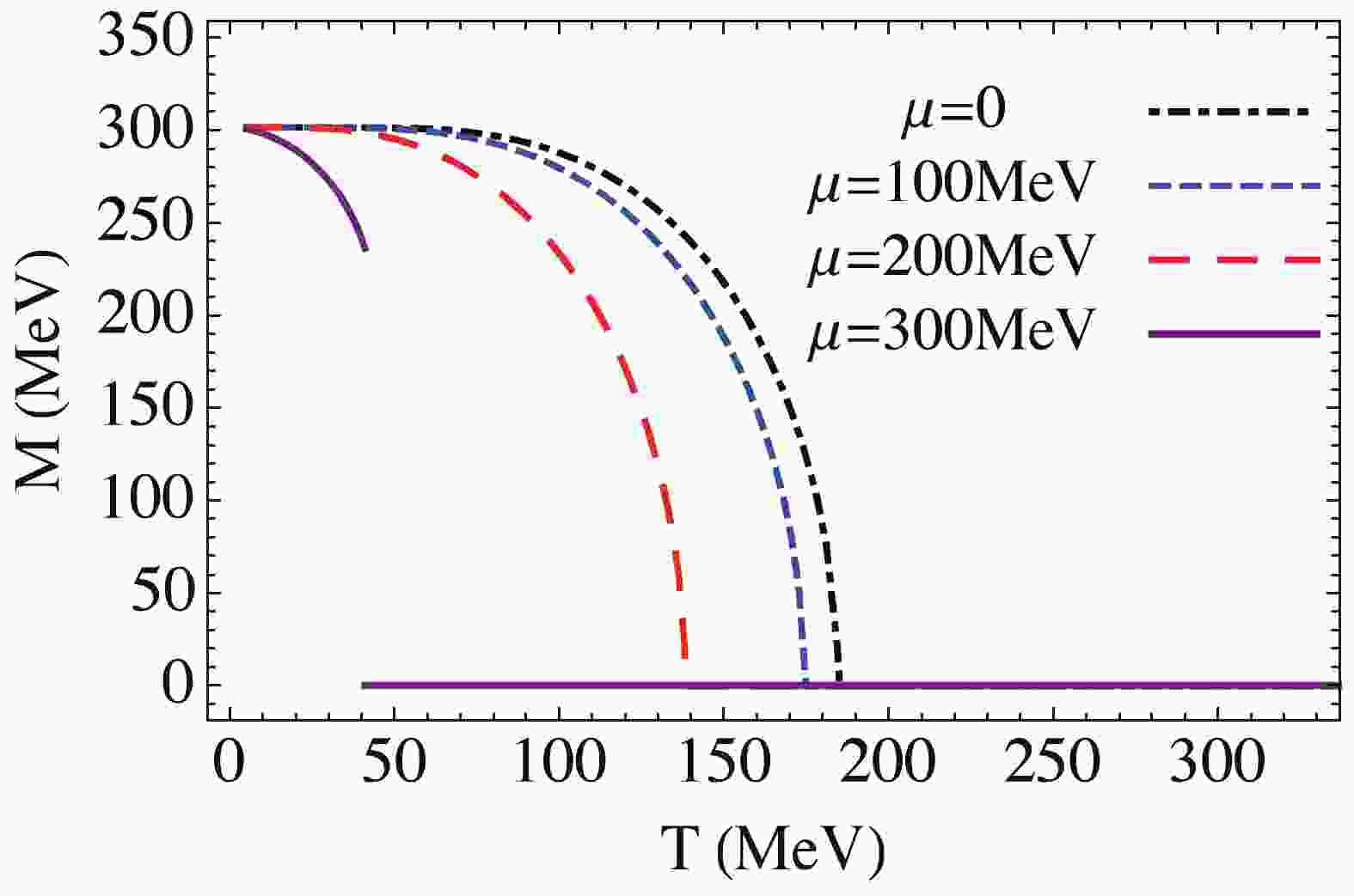
$ f(E) = 1/(1+e^{\beta E}) $ is the Fermi-Dirac distribution. If the phase transition is of first order, the gap equation has multiple solutions. In this case, we compare their grand potentials and find the physical solution of$ \upsilon $ .Figure 1 shows the effective quark mass M as a function of T for various values of the chemical potential
$ \mu $ in the chiral limit ($ m_0 = 0 $ ). Figure 2 shows the well-known phase diagram of the NJL model in the T-$ \mu $ plane. At small chemical potential, the chiral phase transition is of second order. It becomes of first order at large$ \mu $ . Hence, a tricritical point appears. For physical current quark mass, the second-order phase transition turns into a crossover, and the tricritical point becomes a critical endpoint.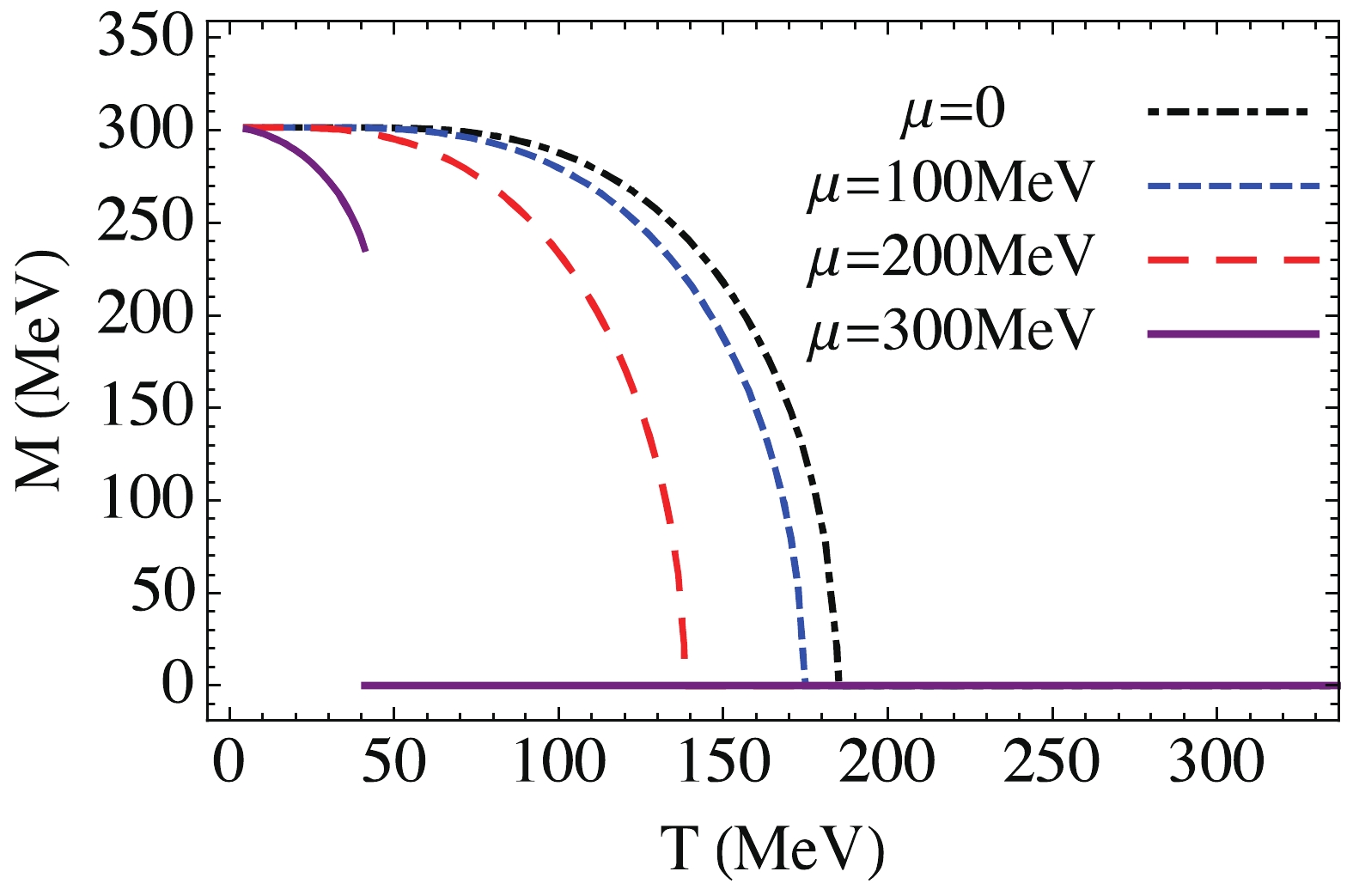
Figure 1. (color online) Effective quark mass M as a function of T for various values of chemical potential
$ \mu $ in chiral limit ($ m_0 = 0 $ ).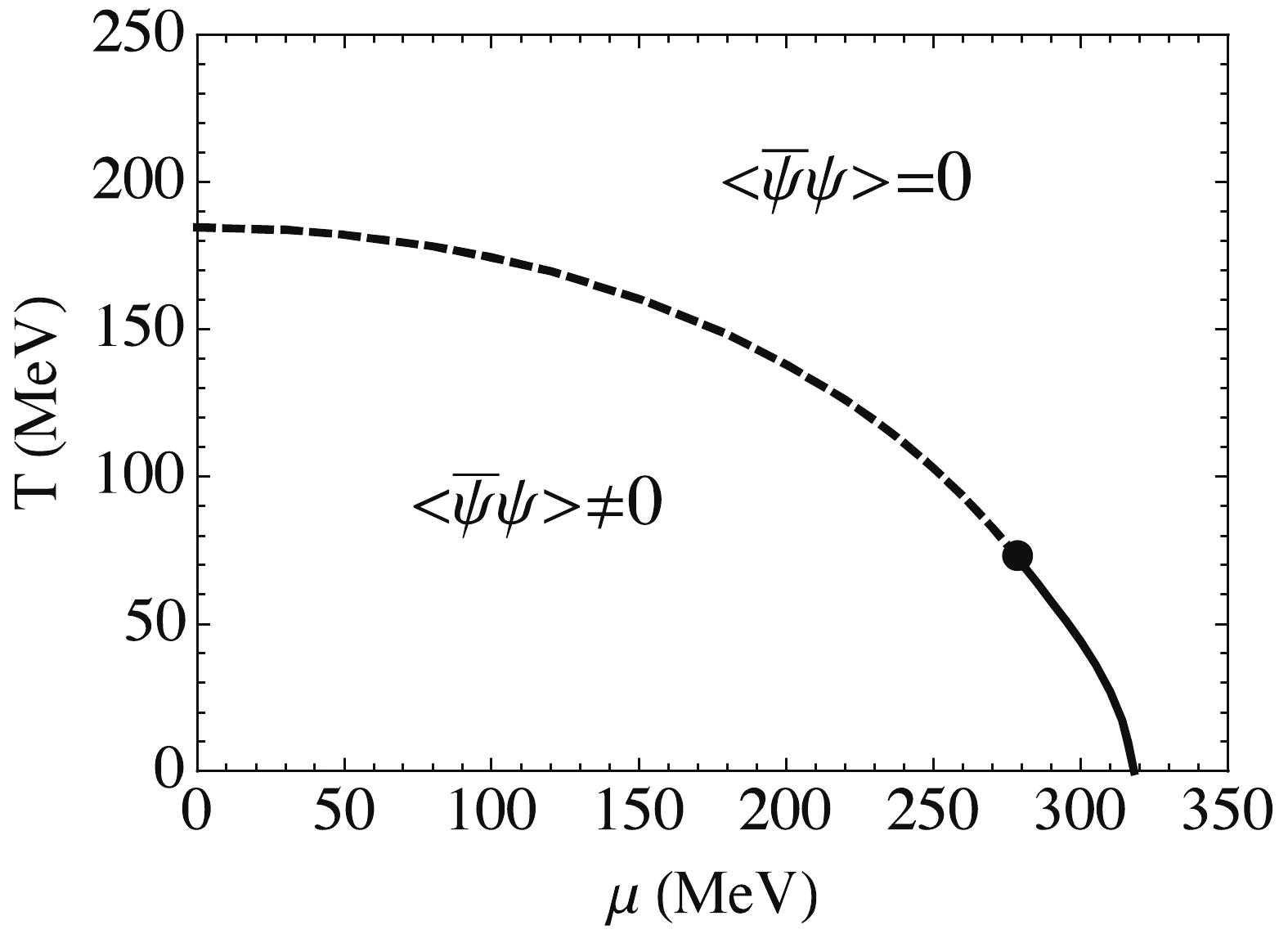
Figure 2. Phase diagram of NJL model in T-
$ \mu $ plane for chiral limit ($ m_0 = 0 $ ). Chiral symmetry broken and restored phases are denoted by$ \langle\bar{\psi}\psi\rangle\neq0 $ and$ \langle\bar{\psi}\psi\rangle = 0 $ , respectively. The dashed and solid lines represent second-order and first-order phase transitions, respectively. -
Here, we include the mesonic degrees of freedom. To this end, we consider the excitations corresponding to the fluctuation fields
$ \sigma(x) $ and$ {{ \pi }}(x) $ . It is convenient to work in the momentum space by defining the Fourier transformation$ \begin{aligned} \phi_{m}(x) = \sum_Q \phi_{m}(Q){\rm e}^{-{\rm i}q_l\tau+{\rm i}{ q}\cdot{ r}},\ \ \ \ \ {m} = 0,1,2,3, \end{aligned} $

(36) where
$ \phi_0 = \sigma $ and$ \phi_{i} = \pi_{i} $ ($ {i} = 1,2,3 $ ). Here$ Q\equiv(iq_l, { q}) $ with$ q_l = 2l\pi T $ ($ l\in\mathbb{Z} $ ) as the boson Matsubara frequency. The notation$ \displaystyle\sum_Q = \displaystyle\sum_l\int\displaystyle\frac{{\rm d}^3{ q}}{(2\pi)^3} $ is used throughout. In the momentum space, the inverse of the quark Green's function$ { G}^{-1} $ reads$ \begin{array}{l} { G}^{-1}(K,K^\prime) = {\cal G}^{-1}(K)\delta_{K,K^\prime}-\Sigma_{\rm FL}(K,K^\prime), \end{array} $

(37) where
$ K = (ik_n, { k}) $ and$ \begin{array}{l} \Sigma_{\rm FL}(K,K^\prime) = \displaystyle\sum_{m = 0}^3\Gamma_{m}\phi_{m}(K-K^\prime). \end{array} $

(38) Here we have defined
$ \Gamma_0 = 1 $ and$ \Gamma_{i} = i\gamma_5\tau_{\rm i} $ ($ {i} = 1,2,3 $ ). Applying the derivative expansion, we obtain$ \begin{split} {\cal S}_{\rm{eff}}^{(2)}[\sigma,{{\pi}}] = \frac{\beta V}{2}\sum_{{m,n} = 0}^3\sum_Q\phi_{m}(-Q)[{ D}^{-1}(Q)]_{mn}\phi_{n}(Q), \end{split} $

(39) where
$ \begin{split} [{ D}^{-1}(Q)]_{mn} = \frac{\delta_{mn}}{2G}+\Pi_{mn}(Q) \end{split} $

(40) is the inverse of the meson Green's function. The polarization function
$ \Pi_{mn}(Q) $ is defined as$ \begin{split} \Pi_{mn}(Q) = \frac{1}{\beta V}\sum_{K}{\rm Tr}\left[{\cal G}(K)\Gamma_{m}{\cal G}(K+Q)\Gamma_{n}\right]. \end{split} $

(41) The notation
$ \sum_K = \displaystyle\sum_n\int\frac{{\rm d}^3{ k}}{(2\pi)^3} $ will be used throughout. Since we consider the case$ \mu_{I} = 0 $ , the off-diagonal components vanishes, i.e.,$ \Pi_{mn}(Q) = \delta_{mn}\Pi_{m}(Q) $ . It is also evident that$ \Pi_{m}(-Q) = \Pi_{m}(Q) $ .The meson polarization functions
$ \Pi_{m}(Q) $ can be evaluated as$ \begin{split} \Pi_{\rm 0}(iq_l,{ q}) =& N_cN_f \int{{\rm d}^3{ k}\over (2\pi)^3}\Bigg[\left(\frac{1-f(E_{ k}^+)-f(E_{{ k}+{ q}}^-)}{iq_l-E_{ k}-E_{{ k}+{ q}}}\right.\\&\left.-\frac{1-f(E_{ k}^-)-f(E_{{ k}+{ q}}^+)}{iq_l+E_{ k}+E_{{ k}+{ q}}}\right) \left(1+\frac{{ k}\cdot ({ k+ q})-M^2}{E_{ k} E_{{ k}+{ q}}}\right)\\ &+\left(\frac{f(E_{ k}^-)-f(E_{{ k}+{ q}}^-)}{iq_l+E_{ k}-E_{{ k}+{ q}}}-\frac{f(E_{ k}^+)-f(E_{{ k}+{ q}}^+)}{iq_l-E_{ k}+E_{{ k}+{ q}}}\right) \\&\times\left(1-\frac{{ k}\cdot ({ k+ q})-M^2}{E_{ k} E_{{ k}+{ q}}}\right)\Bigg] \end{split} $

(42) for
$ {m} = 0 $ , and$ \begin{split} \Pi_{m}(iq_l,{ q}) =& N_cN_f \int{{\rm d}^3{ k}\over (2\pi)^3}\Bigg[\left(\frac{1-f(E_{ k}^+)-f(E_{{ k}+{ q}}^-)}{iq_l-E_{ k}-E_{{ k}+{ q}}}\right.\\&\left.-\frac{1-f(E_{ k}^-)-f(E_{{ k}+{ q}}^+)}{iq_l+E_{ k}+E_{{ k}+{ q}}}\right) \left(1+\frac{{ k}\cdot ({ k+ q})+M^2}{E_{ k} E_{{ k}+{ q}}}\right)\\& +\left(\frac{f(E_{ k}^-)-f(E_{{ k}+{ q}}^-)}{iq_l+E_{ k}-E_{{ k}+{ q}}}-\frac{f(E_{ k}^+)-f(E_{{ k}+{ q}}^+)}{iq_l-E_{ k}+E_{{ k}+{ q}}}\right)\\&\times \left(1-\frac{{ k}\cdot ({ k+ q})+M^2}{E_{ k} E_{{ k}+{ q}}}\right)\Bigg] \end{split} $

(43) for
$ {m} = 1,2,3 $ . Here, we defined$ E_{ k}^\pm = E_{ k}\pm\mu $ for convenience. In the chiral limit, we can show that from the gap equation,$ 1/(2G)+\Pi_{m}(0,0) = 0 $ ($ {m} = 1,2,3 $ ) in the chiral symmetry broken phase$ M\neq0 $ , which manifests the fact that the pions are Goldstone bosons in this phase. In the chiral symmetry restored phase,$ M = 0 $ , we obtain$ \Pi_{\rm 0}(Q) = \Pi_{\rm 1}(Q) = \Pi_{\rm 2}(Q) = \Pi_{\rm 3}(Q) $ , which indicates that the sigma meson and the pions become degenerate.In the Gaussian approximation, the path integral over
$ \phi_{m} $ can be completed. The mesonic contribution to the thermodynamic potential can be evaluated as$ \begin{split} \Omega_{\rm FL} =& \frac{1}{2\beta V}\sum_{Q}\ln\det\left[{ D}^{-1}(Q)\right] \\=& \frac{1}{2}\sum_{{m} = 0}^3\frac{1}{\beta}\sum_l\int\frac{{\rm d}^3{ q}}{(2\pi)^3}\ln\left[\frac{1}{2G}+\Pi_{m}(iq_l,{ q})\right]{\rm e}^{{\rm i}q_l0^+}. \end{split} $

(44) We can convert the summation over the boson Matsubara frequency to an contour integration and obtain [74]
$ \begin{split} \Omega_{\rm FL} = &-\sum_{{m} = 0}^3\int\frac{{\rm d}^3{ q}}{(2\pi)^3}\int_0^\infty\frac{{\rm d}\omega}{2\pi i} \left[\frac{\omega}{2}+\frac{1}{\beta}\ln\left(1-e^{-\beta\omega}\right)\right]\\&\times \frac{{\rm d}}{{\rm d}\omega}\ln\left[\frac{1+2G\Pi_{m}(\omega+i0^+,{ q})}{1+2G\Pi_{m}(\omega-i0^+,{ q})}\right]. \end{split} $

(45) This result could be related to the Bethe-Uhlenbeck expression, i.e., the second virial contribution in terms of the two-body scattering phase shift [74]. We note that
$ 1+2G\Pi_{m}(\omega+i0^+,{ q}) $ is proportional to the T-matrix for the quark-antiquark scattering in the$ {m} $ -channel, with total energy$ \omega $ and momentum$ { q} $ . The scattering matrix element can be written in the Jost representation as$ \begin{split} {\cal S}_{m}(\omega,{ q}) = \frac{1+2G\Pi_{m}(\omega-i0^+,{ q})}{1+2G\Pi_{m}(\omega+i0^+,{ q})}. \end{split} $

(46) The S-matrix element may has poles corresponding to mesonic bound states. Above the threshold for elastic scattering, it can be represented by a scattering phase shift as
$ \begin{array}{l} {\cal S}_{m}(\omega,{ q}) = {\rm e}^{2{\rm i}\phi_{m}(\omega,{ q})}. \end{array} $

(47) Combining a possible pole term and the scattering contribution, we have [74]
$ \begin{split} \Omega_{\rm FL} =& \sum_{{m} = 0}^3\int\frac{{\rm d}^3{ q}}{(2\pi)^3}\int_0^\infty {\rm d}\omega\left[\frac{\omega}{2}+\frac{1}{\beta}\ln\left(1-e^{-\beta\omega}\right)\right] \\&\times\left[\delta(\omega-\varepsilon_{m}({ q}))+\frac{1}{\pi}\frac{\partial \phi_{m}(\omega,{ q})}{\partial \omega}\right], \end{split} $

(48) where the mesonic pole energy can be given by
$ \varepsilon_{m}({ q}) = \sqrt{{ q}^2+m_{m}^2} $ , with the in-medium meson mass$ m_{m} $ . At low temperature, the above expression explicitly recovers the fact that thermodynamic quantities are dominated by the lightest mesonic excitations, i.e., the pions [75]. In the chiral limit, the pressure of the system at low temperature can be well given by the pressure of a gas of noninteracting massless pions,$ p = \pi^2T^4/30 $ . -
We now start to study the linear response of the hot and dense matter in the NJL model, based on the description of the equilibrium thermodynamics in the last section. In this section, we introduce a generic theoretical framework to compute the following imaginary-time-ordered current-current correlation function
$ \begin{array}{l} \Pi^{\mu\nu}(\tau-\tau^\prime,{ r}-{ r}^\prime) = -\left\langle {T}_\tau \left[{J}^\mu(\tau,{ r}){J}^\nu(\tau^\prime,{ r}^\prime)\right]\right\rangle_{c}, \end{array} $

(49) where
$ {J}^\mu(\tau,{ r}) $ can be any current operator. The notation$ \langle \cdots\rangle_{c} $ denotes the connected piece of the correlation function. For a pure fermionic field theory with a Lagrangian density$ \begin{array}{l} {\cal L}[\psi,\bar{\psi}] = \bar\psi(i\gamma^\mu\partial_\mu-m_0)\psi+{\cal L}_{\rm int}[\psi,\bar{\psi}], \end{array} $

(50) the current operator is given by
$ \begin{array}{l} {J}^{\mu} = \bar\psi\Gamma^\mu\psi, \end{array} $

(51) where
$ \Gamma^\mu = \gamma^\mu\hat{X} $ with$ \hat{X} $ depicting any Hermitian matrix in the spin, flavor, and color spaces. For instance, the electromagnetic current is defined by$ \hat{X} = {\rm diag}(2e/3,-e/3) $ in the flavor space with e being the elementary electric charge and$ \hat{X} = \gamma_5 $ in the spin space gives the axial vector current.Parallel to the path integral approach to the equilibrium thermodynamics, we introduce a path integral formalism for the linear response. In this formalism, we introduce an external source term to compute the correlation function
$ \Pi^{\mu\nu}(\tau,{ r}) $ . The external source physically represents an external perturbation applied to the system. The external source here is actually an external gauge field$ A_\mu(\tau,{ r}) $ which couples to the current$ {J}^\mu(\tau,{ r}) $ . We still use$ x = (\tau, { r}) $ for convenience. The partition function with the external source is given by$ \begin{array}{l} {\cal Z}[A] = \displaystyle\int [{\rm d}\psi][{\rm d}\bar{\psi}]\exp\left\{-{\cal S}[\psi,\bar{\psi};A]\right\}, \end{array} $

(52) where the action reads
$ \begin{array}{l} {\cal S}[\psi,\bar{\psi};A] = \displaystyle\int {\rm d}x\ \bigg\{-{\cal L}[\psi,\bar{\psi}]-\mu\bar\psi\gamma^0\psi+A_\mu(x)\bar\psi\Gamma^\mu\psi\bigg\}. \end{array} $

(53) It is convenient to use the generating functional
$ {\cal W}[A] $ defined as$ \begin{array}{l} {\cal Z}[A] = \exp{\Big\{-{\cal W}[A]\Big\}}. \end{array} $

(54) If the the generating functional can be computed exactly, the correlation function is given by
$ \begin{split} \Pi^{\mu\nu}(\tau-\tau^\prime,{ r}-{ r}^\prime) = \frac{\delta^2{\cal W}[A]} {\delta A_\mu(\tau,{ r})\delta A_\nu(\tau^\prime,{ r}^\prime)}\Bigg|_{A = 0}. \end{split} $

(55) In practice, we need to evaluate the generating functional in some approximations. It is convenient to work in the momentum space by making the Fourier transform
$ \begin{array}{l} A_\mu(x) = \sum_Q A_\mu(Q){\rm e}^{-{\rm i}q_l\tau+{\rm i}{ q}\cdot{ r}}. \end{array} $

(56) To evaluate the correlation function, we expand the generating functional
$ {\cal W}[A] $ in powers of$ A_\mu(Q) $ . The expansion can be formally given by$ \begin{array}{l} {\cal W}[A] = {\cal W}^{(0)}+{\cal W}^{(1)}[A]+{\cal W}^{(2)}[A]+\cdots, \end{array} $

(57) where
$ {\cal W}^{(n)} $ is the nth-order expansion in$ A_\mu(Q) $ . The zeroth-order contribution$ {\cal W}^{(0)} $ recovers the equilibrium grand potential$ \Omega $ with a vanishing external source,$ \begin{array}{l} {\cal W}^{(0)} = \beta V\Omega. \end{array} $

(58) The first-order contribution
$ {\cal W}^{(1)}[A] $ provides nothing but the thermodynamic relation for the charge density$ n_{X} = \langle {\rm J}^0\rangle $ . We have$ n_{X} = -\partial\Omega/\partial\mu_{X} $ , where the chemical potential is defined as$ \mu_{X} = A_0(Q = 0) $ . Hence, we have$ \begin{split} \frac{{\cal W}^{(1)}[A]}{\beta V} = -n_{X}A_0(Q = 0). \end{split} $

(59) The second-order contribution
$ {\cal W}^{(2)}[A] $ characterizes the linear response. It can be formally given by$ \begin{split} \frac{{\cal W}^{(2)}[A]}{\beta V} = \frac{1}{2}\sum_Q \Pi^{\mu\nu}(Q)A_\mu(-Q)A_\nu(Q). \end{split} $

(60) Here
$ \Pi^{\mu\nu}(Q) $ is just the correlation function in the momentum space. The static and long-wavelength limit of its$ 00 $ -component,$ \Pi^{00}(Q = 0) $ , is related to to the number susceptibility, i.e.,$ \begin{split} \lim_{{ q}\rightarrow0}\Pi^{00}(iq_l = 0,{ q}) = \frac{\partial^2\Omega(T,\mu_{X})}{\partial \mu_{X}^2}. \end{split} $

(61) For instance, for the vector current with
$ \hat{X} = 1 $ ,$ \Pi^{00}(Q = 0) $ is proportional to the baryon number susceptibility. The above discussions are precise if the generating functional$ {\cal W}[A] $ or its second-order expansion$ {\cal W}^{(2)}[A] $ can be computed exactly.Followingly, we turn to the NJL model. The partition function of the NJL model with the external source is given by
$ \begin{array}{l} {\cal Z}_{\rm NJL}[A] = \displaystyle\int [{\rm d}\psi][{\rm d}\bar{\psi}]\exp\left\{-{\cal S}[\psi,\bar{\psi};A]\right\}, \end{array} $

(62) with the action
$ \begin{array}{l} {\cal S}[\psi,\bar{\psi};A] = \displaystyle\int {\rm d}x\ \bigg\{-{\cal L}_{\rm NJL}[\psi,\bar{\psi}]-\mu\bar\psi\gamma^0\psi+A_\mu(x)\bar\psi\Gamma^\mu\psi\bigg\}. \end{array} $

(63) Again, introducing two auxiliary fields
$ \sigma $ and$ {{ \pi }} $ , which satisfy equations of motion$ \sigma = -2G\bar{\psi}\psi,\;{{ \pi}} = $ $ -2G\bar{\psi}i\gamma_5{{ \tau }}\psi $ , and applying the Hubbard-Strotonovich transformation, we obtain$ \begin{array}{l} {\cal Z}_{\rm NJL}[A] = \displaystyle\int [{\rm d}\psi] [{\rm d}\bar{\psi}] [{\rm d}\sigma] [{\rm d}{{\pi}}]\exp\left\{-{\cal S}[\psi,\bar{\psi},\sigma,{{\pi}};A]\right\}, \end{array} $

(64) where the action now reads
$ \begin{split} {\cal S}[\psi,\bar{\psi},\sigma,{{\pi}};A] =& \int {\rm d}x \frac{\sigma^2(x)+{{\pi}}^2(x)}{4G}\\&-\int {\rm d}x\int {\rm d}x^\prime\bar{\psi}(x){ G}_{A}^{-1}(x,x^\prime)\psi(x^\prime), \end{split} $

(65) with the inverse of the fermion Green's function
$ \begin{split} { G}_{A}^{-1}(x,x^\prime) =& \Big\{\gamma^0(-\partial_\tau+\mu)+i{{\gamma}}\cdot{{\nabla}}-m_0 -\left[\sigma(x)+i\gamma_5{{\tau}}\cdot{{\pi}}(x)\right]\\&-\Gamma^\mu A_\mu(x)\Big\}\delta(x-x^\prime). \end{split} $

(66) Integrating out the quark field yields
$ \begin{split} {\cal Z}_{\rm NJL}[A] =& \int [{\rm d}\sigma][{\rm d}{{\pi}}] \exp\left\{-{\cal S}_{\rm{eff}}[\sigma,{{\pi}};A]\right\},\\ {\cal S}_{\rm{eff}}[\sigma,{{\pi}};A] =& \int {\rm d}x\frac{\sigma^2(x)+{{\pi}}^2(x)}{4G}-{\rm Tr}\ln{ G}_{A}^{-1}(x,x^\prime). \end{split} $

(67) The treatment of the the expectation values of the meson fields
$ \sigma(x) $ and$ {{ \pi }}(x) $ , or their classical fields$ \sigma_{cl}(x) $ and$ {{ \pi }}_{cl}(x) $ , becomes nontrivial. In the absence of the external source, we choose$ \sigma_{cl}(x) = \upsilon $ and$ {{\pi }}_{cl}(x) = 0 $ , which are static and homogeneous. However, in the absence of the external source, they are generally no longer static and homogeneous. Again, we apply the field shifts,$\sigma(x)\rightarrow $ $ \sigma_{cl}(x)+\sigma(x) $ and$ {{ \pi }}(x)\rightarrow{{ \pi }}_{cl}(x)+{{ \pi }}(x) $ , and expand the effective action$ {\cal S}_{\rm{eff}}[\sigma,{{ \pi }}] $ in powers of the fluctuations$ \sigma(x) $ and$ {{ \pi }}(x) $ . We obtain$ \begin{array}{l} {\cal S}_{\rm{eff}}[\sigma,{{\pi}};A] = {\cal S}_{\rm{eff}}^{(0)}[A]+{\cal S}_{\rm{eff}}^{(1)}[\sigma,{{\pi}};A] +{\cal S}_{\rm{eff}}^{(2)}[\sigma,{{\pi}};A]+\cdots. \end{array} $

(68) Parallel to the case without external source, we neglect the mesonic fluctuations of order higher than the Gaussian. The linear term
$ {\cal S}_{\rm{eff}}^{(1)}[\sigma,{{ \pi }};A] $ can be shown to vanish once the classical fields$ \sigma_{cl}(x) $ and$ {{ \pi }}_{cl}(x) $ are determined by minimizing$ {\cal S}_{\rm{eff}}^{(0)}[A] $ . The partition function in the Gaussian approximation is given by$ \begin{array}{l} {\cal Z}_{\rm NJL}\approx\exp\left\{-{\cal S}_{\rm{eff}}^{(0)}[A]\right\}\displaystyle\int [{\rm d}\sigma][{\rm d}{{\pi}}] \exp\left\{-{\cal S}_{\rm{eff}}^{(2)}[\sigma,{{\pi}};A]\right\}. \end{array} $

(69) Therefore, in this Gaussian approximation, the generating functional
$ {\cal W}_{\rm NJL}[A] $ includes both the mean-field (MF) and the meson-fluctuation (FL) contributions. We have$ \begin{array}{l} {\cal W}_{\rm NJL}[A] = {\cal W}_{\rm MF}[A]+{\cal W}_{\rm FL}[A], \end{array} $

(70) where
$ \begin{split} {\cal W}_{\rm MF}[A] =& {\cal S}_{\rm{eff}}^{(0)}[A],\\ {\cal W}_{\rm FL}[A] =& -\ln\left[\int [{\rm d}\sigma][{\rm d}{{\pi}}] \exp\left\{-{\cal S}_{\rm{eff}}^{(2)}[\sigma,{{\pi}};A]\right\}\right]. \end{split} $

(71) In the path integral, we can treat the equilibrium thermodynamics and the linear response at the same footing. The mean-field and the meson-fluctuation contributions to the generating functional can be expanded in powers of the external source as
$ \begin{split} {\cal W}_{\rm MF}[A] =& {\cal W}_{\rm MF}^{(0)}+{\cal W}_{\rm MF}^{(1)}[A]+{\cal W}_{\rm MF}^{(2)}[A]+\cdots,\\ {\cal W}_{\rm FL}[A] =& {\cal W}_{\rm FL}^{(0)}+{\cal W}_{\rm FL}^{(1)}[A]+{\cal W}_{\rm FL}^{(2)}[A]+\cdots. \end{split} $

(72) The zeroth-order contributions recover the equilibrium thermodynamic potentials, i.e.,
$ {\cal W}_{\rm MF}^{(0)} = \beta V \Omega_{\rm MF} $ and$ {\cal W}_{\rm FL}^{(0)} = \beta V \Omega_{\rm FL} $ .So far, the dependence on the classical fields
$ \sigma_{cl}(x) $ and$ {{ \pi }}_{cl}(x) $ is not explicitly shown. They are not independent quantities and should be determined as functionals of the external source via some gap equations. We write$ \begin{array}{l} {\cal W}_{\rm NJL}[A] = {\cal W}_{\rm MF}[A;\sigma_{cl}, {{\pi}}_{cl}]+{\cal W}_{\rm FL}[A;\sigma_{cl}, {{\pi}}_{cl}]. \end{array} $

(73) Parallel to the theory of the equilibrium thermodynamics, we require that the classical fields are determined by minimizing the mean-field part of the generating functional, i.e.,
$ \begin{split} \frac{\delta{\cal W}_{\rm MF}[A;\sigma_{cl}, {{\pi}}_{cl}]}{\delta\sigma_{cl}(x)} =& 0,\\ \frac{\delta{\cal W}_{\rm MF}[A;\sigma_{cl}, {{\pi}}_{cl}]}{\delta{{\pi}}_{cl}(x)} =& 0. \end{split} $

(74) Once this extreme condition is imposed, we can show that the linear term
$ {\cal S}_{\rm{eff}}^{(1)}[\sigma,{{ \pi }};A] $ vanishes exactly. Moreover, it is also necessary to maintain the Goldstone's theorem. Solving the extreme condition formally, we have$ \begin{array}{l} \sigma_{cl}(x) = F_\sigma[A],\ \ \ \ \ \ {{\pi}}_{cl}(x) = { F}_\pi[A]. \end{array} $

(75) Substituting these solutions into the generating functional, we finally eliminate the dependence on the classical fields.
In the following sections, we will study the response functions in the mean-field approximation (
${\cal S}_{\rm{eff}}\simeq{\cal S}_{\rm{eff}}^{(0)}, $ $ {\cal W}_{\rm NJL}\simeq{\cal W}_{\rm MF} $ ) and in the Gaussian-fluctuation approximation ($ {\cal S}_{\rm{eff}}\simeq{\cal S}_{\rm{eff}}^{(0)}+{\cal S}_{\rm{eff}}^{(2)},{\cal W}_{\rm NJL}\simeq{\cal W}_{\rm MF}+{\cal W}_{\rm FL} $ ). Here, we have truncated the mesonic fluctuations up to the quadratic order, since higher-order contributions cannot be analytically treated. The mean-field truncation, corresponding to the random phase approximation of the linear response, is obviously self-consistent, as has been verified in numerous studies of the many-body theory. The Gaussian-fluctuation truncation takes into account the contribution from the collective modes (mesons). The contributions higher than the Gaussian may correspond to the interaction between mesons, which are assumed to be weak and therefore can be neglected. However, one can show that the Gaussian-fluctuation approximation also preserves the Ward-Takahashi identity and hence the conservation laws [97-99]. In the context of the electromagnetic response of superconductors, such a Gaussian-fluctuation approximation leads to a gauge invariant linear response theory [97-99]. -
We first present the linear response in the mean-field approximation, i.e.,
$ {\cal W}_{\rm NJL}[A] \simeq {\cal W}_{\rm MF}[A] $ . We will see that the response functions in this approximation recovers the famous random phase approximation (RPA) developed in early condensed matter theory. Since we are interested in the response to an infinitesimal external source, we expect that the induced perturbations to the classical fields are also infinitesimal. Therefore, we have$ \begin{array}{l} \sigma_{cl}(x) = \upsilon+\eta_0(x),\ \ \ \ \ {{\pi}}_{cl}(x) = 0+{{\eta}}(x), \end{array} $

(76) where the static and uniform part
$ \upsilon $ is the chiral condensate with vanishing external source. The generating functional in the mean-field approximation is given by$ \begin{split} {\cal W}_{\rm MF}[A;\sigma_{cl}, {{\pi}}_{cl}] =& \int {\rm d}x \frac{\sigma_{cl}^2(x)+{{\pi}}^2_{cl}(x)}{4G} \\&- {\rm Tr\, ln}\left[{\cal G}_{A}^{-1}(x,x^\prime)\right]. \end{split} $

(77) Here
$ {\cal G}_{A}^{-1} $ is the inverse of the fermion Green's function in the mean-field approximation with external source. It can be expressed as$ \begin{array}{l} {\cal G}_{A}^{-1}(x,x^\prime) = {\cal G}^{-1}(x,x^\prime)-\Sigma_{\rm A}(x,x^\prime), \end{array} $

(78) where the two terms are defined as
$ \begin{split} {\cal G}^{-1}(x,x^\prime) = \left[\gamma^0(-\partial_\tau+\mu)+i{{\gamma}}\cdot{{\nabla}}-M\right]\delta(x-x^\prime), \end{split} $

$ \begin{split} \Sigma_{A}(x,x^\prime) = \left[\sum_{m = 0}^3\Gamma_{m}\eta_{m}(x)+\Gamma^\mu A_\mu(x)\right]\delta(x-x^\prime). \end{split} $

(79) Here
$ M = m_0+\upsilon $ is the effective quark mass as we have defined in the absence of the external source.Now we turn to the momentum space via the Fourier transform
$ \begin{split} \eta_{m}(x) = \sum_Q \eta_{m}(Q){\rm e}^{-{\rm i}q_l\tau+{\rm i}{ q}\cdot{ r}}. \end{split} $

(80) In the momentum space, the inverse of the fermion Green's function is given by
$ \begin{array}{l} {\cal G}_{A}^{-1}(K,K^\prime) = {\cal G}^{-1}(K)\delta_{K,K^\prime}-\Sigma_{A}(K,K^\prime), \end{array} $

(81) where
$ {\cal G}^{-1}(K) $ is given by (33) and$ \begin{split} \Sigma_{A}(K,K^\prime) = \sum_{m = 0}^3\Gamma_{m}\eta_{m}(K-K^\prime)+\Gamma^\mu A_\mu(K-K^\prime). \end{split} $

(82) Using the derivative expansion, we can expand the generating functional in powers of the external source as well as the induced perturbations
$ \eta_{m} $ . We have$ \begin{array}{l} {\cal W}_{\rm MF}[A;\eta] = {\cal W}_{\rm MF}^{(0)}+{\cal W}_{\rm MF}^{(1)}[A;\eta]+{\cal W}_{\rm MF}^{(2)}[A;\eta]+\cdots, \end{array} $

(83) where it is obvious that
$ {\cal W}_{\rm MF}^{(0)} = \beta V\Omega_{\rm MF} $ . Note that the induced perturbation should be finally eliminated via the gap equation (74).The linear term
$ {\cal W}_{\rm MF}^{(1)}[A;\eta] $ can be evaluated as$ \begin{split} \frac{{\cal W}_{\rm MF}^{(1)}[A;\eta]}{\beta V} =& \left[\frac{\upsilon}{2G}+\frac{1}{\beta V}\sum_K{\rm Tr}{\cal G}(K)\right]\eta_0(0) \\&+\frac{1}{\beta V}\sum_K{\rm Tr}\left[{\cal G}(K)i\gamma^5{{\tau}}\right]\cdot{{\eta}}(0) \\&+\frac{1}{\beta V}\sum_K{\rm Tr}\left[{\cal G}(K)\Gamma^\mu\right] A_\mu(0). \end{split} $

(84) It is related only to the
$ Q = 0 $ component of the external source and the induced perturbations. The explicit form of$ {\cal G}(K) $ can be evaluated as$ \begin{split} {\cal G}(K) = \frac{1}{ik_n-E_{ k}} \Lambda_{+}({ k})\gamma_0 + \frac{1}{ik_n+E_{ k}} \Lambda_{-}({ k})\gamma_0, \end{split} $

(85) where the the energy projectors
$ \Lambda_\pm({ k}) $ are given by$ \begin{split} \Lambda_{\pm}({ k}) = \frac{1}{2}\left[1\pm{\gamma_0\left({{\gamma}}\cdot{ k}+M\right)\over E_{ k}} \right]. \end{split} $

(86) Using the gap equation (35), we can show that the only nonvanishing part is related to the number density, i.e.,
$ \begin{split} \frac{{\cal W}_{\rm MF}^{(1)}[A;\eta]}{\beta V} = -(n_{X})_{\rm MF}A_0(0), \end{split} $

(87) where the number density is given by
$ \begin{split} (n_{X})_{\rm MF} = \frac{1}{\beta V}\sum_K{\rm Tr}\left[{\cal G}(K)\Gamma^0\right]. \end{split} $

(88) It is evident that
$ (n_{X})_{\rm MF} = -\partial\Omega_{\rm MF}/\partial\mu_{X} $ with the chemical potential$ \mu_{X} = A_0(0) $ .The linear response is characterized by the quadratic term
$ {\cal W}_{\rm MF}^{(2)}[A;\eta] $ . By making use of the derivative expansion and completing the trace in the momentum space, we obtain$ \begin{split} {\cal W}_{\rm MF}^{(2)}[A;\eta] =& \frac{\beta V}{4G}\sum_{m = 0}^3\sum_Q\eta_{m}(-Q)\eta_{m}(Q)\\&+\frac{1}{2}\sum_{K}\sum_{K^\prime}{\rm Tr} \left[{\cal G}(K)\Sigma_{\rm A}(K,K^\prime){\cal G}(K^\prime)\Sigma_{\rm A}(K^\prime,K)\right]. \end{split} $

(89) Defining
$ Q = K^\prime-K $ , we obtain$ \begin{split} \frac{{\cal W}_{\rm MF}^{(2)}[A;\eta]}{\beta V} =& \frac{1}{2}\sum_{Q}\Pi_{\rm b}^{\mu\nu}(Q)A_\mu(-Q)A_\nu(Q) \\&+\frac{1}{2}\sum_{m = 0}^3\sum_{Q}\left[\frac{1}{2G}+\Pi_{m}(Q)\right]\eta_{m}(-Q)\eta_{m}(Q)\\ &+\sum_{m = 0}^3\sum_{Q}C^{\mu}_{m}(Q)A_\mu(-Q)\eta_{m}(Q). \end{split} $

(90) Here the the bare response function
$ \Pi_{\rm b}^{\mu\nu}(Q) $ is defined as$ \begin{split} \Pi_{b}^{\mu\nu}(Q) = \frac{1}{\beta V}\sum_{K}{\rm Tr}\left[{\cal G}(K)\Gamma^\mu{\cal G}(K+Q)\Gamma^\nu\right] \end{split} $

(91) and the coupling function
$ C^\mu_{m}(Q) $ is given by$ \begin{split} C^\mu_{m}(Q) = \frac{1}{\beta V}\sum_{K}{\rm Tr}\left[{\cal G}(K)\Gamma^\mu{\cal G}(K+Q)\Gamma_{m}\right]. \end{split} $

(92) The meson polarization functions
$ \Pi_{m}(Q) $ are given in Sec. 3.The final task is to eliminate the induced perturbations. For the purpose of linear response, the induced perturbations
$ \eta_{m}(Q) $ can be determined by$ \begin{split} \frac{\delta{\cal W}_{\rm MF}^{(2)}[A;\eta]}{\delta \eta_{m}(Q)} = 0. \end{split} $

(93) Using the explicit form of
$ {\cal W}_{\rm MF}^{(2)}[A;\eta] $ , we obtain$ \begin{split} \eta_{m}(Q) =& -\frac{C^\mu_{m}(-Q)A_\mu(Q)}{\displaystyle\frac{1}{2G}+\Pi_{m}(Q)}+O(A^2),\\ \eta_{m}(-Q) =& -\frac{C^\mu_{m}(Q)A_\mu(-Q)}{\displaystyle\frac{1}{2G}+\Pi_{m}(Q)}+O(A^2), \end{split} $

(94) where we have applied the fact that
$ \Pi_{m}(-Q) = \Pi_{m}(Q) $ . Using the above results to eliminate the induced perturbations, we finally obtain$ \begin{split} \frac{{\cal W}_{\rm MF}^{(2)}[A]}{\beta V} = \frac{1}{2}\sum_{Q}\Pi_{\rm MF}^{\mu\nu}(Q)A_\mu(-Q)A_\nu(Q), \end{split} $

(95) where the full response function in the mean-field theory reads
$ \begin{split} \Pi_{\rm MF}^{\mu\nu}(Q) = \Pi_{b}^{\mu\nu}(Q)-\sum_{m = 0}^3\frac{C^\mu_{m}(Q)C^\nu_{m}(-Q)}{\displaystyle\frac{1}{2G}+\Pi_{m}(Q)}. \end{split} $

(96) This result recovers nothing but the quasi-particle random phase approximation widely used in condensed matter theory [81]. We note that in addition to the pure quasi-particle contribution
$ \Pi_{b}^{\mu\nu}(Q) $ , the linear response can couple to the collective mesonic modes once$ C^\mu_{m}(Q)\neq0 $ . Hence, the response function reveals meson properties and also possibly phase transitions.In the chiral limit (
$ m_0 = 0 $ ), we can show that$ C^\mu_{m}(Q) = 0 $ in the chiral symmetry restored phase ($ T>T_c $ ). In this case, the quasi-particle random phase approximation just describes the linear response of a hot and dense gas of non-interacting quarks. This is obviously inadequate. We will discuss the linear response theory beyond the quasi-particle random phase approximation in Sec. 7. -
As an application of the mean-field theory or the random phase approximation, we study the linear responses to some density perturbations. To be specific, we consider the following
$ \hat{X} $ operators: (1)$ \hat{X} = 1 $ , corresponding to the vector current; (2)$ \hat{X} = \tau_3 $ , corresponding to the isospin vector current; (3)$ \hat{X} = \gamma_5 $ , corresponding to the axial vector current; (4)$ \hat{X} = \tau_3\gamma_5 $ , corresponding to the isospin axial vector current. The$ 0 $ -component of the current$ {J}^\mu $ is related to the baryon density, isospin density, axial baryon density, and axial isospin density, respectively. The density response function$ \chi(iq_l,{ q}) $ is given by the$ 00 $ -component of the response function$ \Pi^{\mu\nu}(Q) $ . In the mean-field theory, it is given by$ \begin{split} \chi(iq_l,{ q}) = \Pi_{\rm MF}^{00}(Q) = \Pi_{\rm b}^{00}(Q)-\sum_{m = 0}^3\frac{C^0_{m}(Q)C^0_{m}(-Q)}{\displaystyle\frac{1}{2G}+\Pi_{m}(Q)}. \end{split} $

(97) In practice, we define the dynamic structure factor
$ S(\omega,{ q}) $ , which is related to the density response function$ \chi(iq_l,{ q}) $ via the fluctuation-dissipation theorem. It is defined as$ \begin{split} S(\omega,{ q}) = -\frac{1}{\pi}\frac{1}{1-e^{-\beta\omega}}{\rm Im}\chi(\omega+i\epsilon,{ q}). \end{split} $

(98) In the following, we are interested in the long-wavelength limit
$ { q} = 0 $ and focus on the pure dynamical effect. -
For the vector current
$ \hat{X} = 1 $ , the bare response function is given by$ \begin{split} \Pi_{b}^{00}(Q) = \frac{1}{\beta V}\sum_{K}{\rm Tr}\left[{\cal G}(K)\gamma^0{\cal G}(K+Q)\gamma^0 \right]. \end{split} $

(99) At
$ { q} = 0 $ , we can show that$ \Pi_{b}^{00}(iq_l, { q} = 0) $ vanishes. The coupling function is given by$ \begin{split} C^0_{m}(Q) = \frac{1}{\beta V}\sum_{K}{\rm Tr}\left[{\cal G}(K)\gamma^0{\cal G}(K+Q)\Gamma_{m}\right]. \end{split} $

(100) At
$ { q} = 0 $ , we can show that$ C^0_{m}(iq_l, { q} = 0) $ vanish for all$ {m} = 0,1,2,3 $ . Therefore, for the baryon density response, the dynamic structure factor vanishes at$ { q} = 0 $ , i.e.,$ \begin{array}{l} S(\omega,{ q} = 0) = 0. \end{array} $

(101) -
For the isospin vector current
$ \hat{X} = \tau_3 $ , the bare response function is given by$ \begin{split} \Pi_{b}^{00}(Q) = \frac{1}{\beta V}\sum_{K}{\rm Tr}\left[{\cal G}(K)\gamma^0\tau_3{\cal G}(K+Q)\gamma^0 \tau_3\right]. \end{split} $

(102) At
$ { q} = 0 $ , we can show that$ \Pi_{\rm b}^{00}(iq_l, { q} = 0) $ vanishes. The coupling function is given by$ \begin{split} C^0_{m}(Q) = \frac{1}{\beta V}\sum_{K}{\rm Tr}\left[{\cal G}(K)\gamma^0\tau_3{\cal G}(K+Q)\Gamma_{m}\right]. \end{split} $

(103) At
$ { q} = 0 $ , we can show that$ C^0_{m}(iq_l, { q} = 0) $ vanish for all$ {\rm m} = 0,1,2,3 $ . Therefore, for the isospin density response, the dynamic structure factor also vanishes at$ { q} = 0 $ , i.e.,$ \begin{array}{l} S(\omega,{ q} = 0) = 0. \end{array} $

(104) -
For the axial vector current
$ \hat{X} = \gamma_5 $ , the bare response function is given by$ \begin{split} \Pi_{b}^{00}(Q) = \frac{1}{\beta V}\sum_{K}{\rm Tr}\left[{\cal G}(K)\gamma^0\gamma_5{\cal G}(K+Q)\gamma^0 \gamma_5\right]. \end{split} $

(105) Completing the trace and the Matsubara sum, we obtain
$ \begin{split} \Pi_{b}^{00}(iq_l, { q} = 0) =& 2N_c N_f\int{{\rm d}^3{ k}\over (2\pi)^3} \frac{M^2}{E_{ k}^2}\left(\frac{1}{iq_l-2E_{ k}}-\frac{1}{iq_l+2E_{ k}}\right)\\&\times\left[1-f(E_{ k}-\mu)-f(E_{ k}+\mu)\right]. \end{split} $

(106) The coupling function is given by
$ \begin{split} C^0_{m}(Q) = \frac{1}{\beta V}\sum_{K}{\rm Tr}\left[{\cal G}(K)\gamma^0 \gamma^5{\cal G}(K+Q)\Gamma_{m}\right]. \end{split} $

(107) At
$ { q} = 0 $ , we can show that$ C^0_{m}(iq_l, { q} = 0) $ vanish for all$ {\rm m} = 0,1,2,3 $ . Therefore, the axial baryon density response has a nonzero dynamical structure factor at$ { q} = 0 $ . It does not couple to the mesonic modes and is given by$ \chi(iq_l,{ q} = 0) = \Pi_{\rm b}^{00}(iq_l,{ q} = 0) $ . The dynamical structure factor reads$ \begin{split} S(\omega,{ q} = 0) =& N_cN_f \frac{M^2}{2\pi^2} \frac{ \sqrt{\omega^2-4M^2}}{\omega}\frac{\Theta(|\omega|-2M)}{1-e^{-\beta\omega}}\\&\times \left[1-\frac{1}{e^{\beta(\frac{1}{2}\omega-\mu)}+1}-\frac{1}{e^{\beta(\frac{1}{2}\omega+\mu)}+1}\right]. \end{split} $

(108) We note that a similar result was also obtained in Ref. [100]. It is evident that the dynamical structure factor for the axial baryon density response is a direct reflection of the quark mass gap.
$ S(\omega,{ q} = 0) $ is nonzero only for$ |\omega| $ larger than two times the quark mass gap. Figure 3 shows the dynamical structure factor$ S(\omega,{ q} = 0) $ for various values of the temperature. With increasing temperature, the threshold$ \omega_{\rm th} = 2M $ becomes smaller, and finally$ \omega_{\rm th}\rightarrow 0 $ in the high T limit.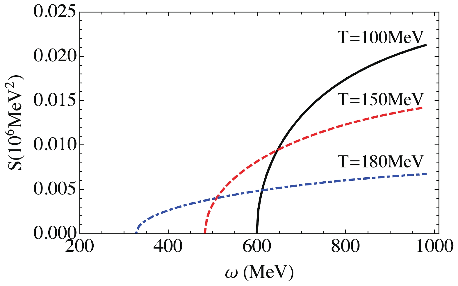
Figure 3. (color online) Dynamical structure factor
$ S(\omega,{ q}) $ at$ { q} = 0 $ for axial baryon density response ($ \hat{X} = \gamma_5 $ ) at various values of T and at$ \mu = 0 $ . We consider the physical current quark mass$ m_0 = 5 $ MeV. -
For the isospin axial vector current
$ \hat{X} = \tau_3\gamma^5 $ , the bare response function is given by$ \begin{split} \Pi_{b}^{00}(Q) = \frac{1}{\beta V}\sum_{K}{\rm Tr}\left[{\cal G}(K)\gamma^0\tau_3\gamma^5{\cal G}(K+Q)\gamma^0 \tau_3\gamma^5\right]. \end{split} $

(109) Completing the trace and the Matsubara sum, we obtain
$ \begin{split} \Pi_{\rm b}^{00}(iq_l, { q} = 0) =& 2N_c N_f\int{{\rm d}^3{ k}\over (2\pi)^3} \frac{M^2}{E_{ k}^2}\left(\frac{1}{iq_l-2E_{ k}}-\frac{1}{iq_l+2E_{ k}}\right)\\&\times\left[1-f(E_{ k}-\mu)-f(E_{ k}+\mu)\right]. \end{split} $

(110) The coupling function is given by
$ \begin{split} C^0_{m}(Q) = \frac{1}{\beta V}\sum_{K}{\rm Tr}\left[{\cal G}(K)\gamma^0 \tau_3\gamma^5{\cal G}(K+Q)\Gamma_{m}\right]. \end{split} $

(111) At
$ { q} = 0 $ , we can show that$ C^0_{m}(iq_l, { q} = 0) $ vanish for$ {m} = 0,1,2 $ . The nonzero coupling$ C^0_{\rm 3}(iq_l, { q} = 0) $ is given by$ \begin{split} C^0_{\rm 3}(iq_l, { q} = 0) =& 2iN_c N_f\int{{\rm d}^3{ k}\over (2\pi)^3} \frac{M}{E_{ k}} \left(\frac{1}{iq_l-2E_{ k}}+\frac{1}{iq_l+2E_{ k}}\right)\\&\times\left[1-f(E_{ k}-\mu)-f(E_{ k}+\mu)\right]. \end{split} $

(112) Thus, the axial isospin density response couples to the neutral pion mode
$ \pi_0 $ .The full response function reads
$ \begin{split} \chi(iq_l,{ q} = 0) =& \Pi_{b}^{00}(iq_l,{ q} = 0)\\&-\frac{C^0_{\rm 3}(iq_l,{ q} = 0)C^0_{\rm 3}(-iq_l,{ q} = 0)}{\displaystyle\frac{1}{2G}+\Pi_{\rm 3}(iq_l,{ q} = 0)}. \end{split} $

(113) Here
$ \Pi_{\rm 3}(iq_l,{ q} = 0) $ is given by$ \begin{split} \Pi_{\rm 3}(iq_l,{ q} = 0) =& 2N_c N_f\int{{\rm d}^3{ k}\over (2\pi)^3}\left(\frac{1}{iq_l-2E_{ k}}-\frac{1}{iq_l+2E_{ k}}\right)\\&\times\left[1-f(E_{ k}-\mu)-f(E_{ k}+\mu)\right]. \end{split} $

(114) To evaluate the dynamical structure factor, we make use of the following results,
$ \begin{split} {\rm Im}\Pi_{\rm b}^{00}(\omega+i\epsilon,{ q} = 0) =& -N_c N_f \frac{M^2}{2\pi}\frac{\sqrt{\omega^2-4M^2}}{\omega}\Theta(|\omega|-2M) \left[1-\frac{1}{e^{\beta(\frac{1}{2}\omega-\mu)}+1}-\frac{1}{e^{\beta(\frac{1}{2}\omega+\mu)}+1}\right],\\ {\rm Re}\Pi_{\rm 3}(\omega+i\epsilon,{ q} = 0) =& 2N_c N_f {\cal P}\int{{\rm d}^3{ k}\over (2\pi)^3}\left(\frac{1}{\omega-2E_{ k}}-\frac{1}{\omega+2E_{ k}}\right)\left[1-f(E_{ k}-\mu)-f(E_{ k}+\mu)\right],\\ {\rm Im}\Pi_{\rm 3}(\omega+i\epsilon,{ q} = 0) =& -N_c N_f \frac{\omega\sqrt{\omega^2-4M^2}}{8\pi} \Theta(|\omega|-2M) \left[1-\frac{1}{e^{\beta(\frac{1}{2}\omega-\mu)}+1}-\frac{1}{e^{\beta(\frac{1}{2}\omega+\mu)}+1}\right],\\ {\rm Re}C^0_{\rm 3}(\omega+i\epsilon,{ q} = 0) =& N_c N_f \frac{M\sqrt{\omega^2-4M^2}}{4 \pi} \Theta(|\omega|-2M){\rm sgn}(\omega) \left[1-\frac{1}{e^{\beta(\frac{1}{2}\omega-\mu)}+1}-\frac{1}{e^{\beta(\frac{1}{2}\omega+\mu)}+1}\right],\\ {\rm Im}C^0_{\rm 3}(\omega+i\epsilon, { q} = 0) =& 2N_c N_f{\cal P}\int{{\rm d}^3{ k}\over (2\pi)^3} \frac{M}{E_{ k}} \left(\frac{1}{\omega-2E_{ k}}+\frac{1}{\omega+2E_{ k}}\right)\left[1-f(E_{ k}-\mu)-f(E_{ k}+\mu)\right]. \end{split} $

(115) Here
$ {\cal P} $ denotes the principal value. The imaginary part of$ \chi(\omega+i\epsilon,{ q} = 0) $ can be expressed as$ \begin{split} {\rm Im}\chi(\omega+i\epsilon) =& \frac{{\rm Im}\Pi_{\rm 3}(\omega+i\epsilon)}{\left[\dfrac{1}{2G}+{\rm Re}\Pi_{\rm 3}(\omega+i\epsilon)\right]^2+\left[{\rm Im}\Pi_{\rm 3}(\omega+i\epsilon)\right]^2}\\&\times \left[{\rm Im}C^0_{\rm 3}(\omega+i\epsilon)-\frac{2M}{\omega}\left(\frac{1}{2G}+{\rm Re}\Pi_{\rm 3}(\omega+i\epsilon)\right)\right]^2. \end{split} $

(116) Here, we have suppressed the condition
$ { q} = 0 $ for convenience. Therefore, we expect that at low temperature, the dynamical structure factor for the axial isospin density response reveals a pole plus continuum structure. For$ |\omega|>2M $ ,$ {\rm Im}\Pi_{\rm 3}(\omega+i\epsilon) $ is nonzero, and hence the dynamical structure factor shows a continuum. For$ |\omega|<2M $ ,$ {\rm Im}\Pi_{\rm 3}(\omega+i\epsilon) $ vanishes and thus the dynamical structure factor is simply proportional to a delta function. We have$ \begin{array}{l} {\rm Im}\chi(\omega+i\epsilon) = \pi\left[{\rm Im}C^0_{\rm 3}(\omega+i\epsilon)\right]^2 \delta{\left(\displaystyle\frac{1}{2G}+{\rm Re}\Pi_{\rm 3}(\omega+i\epsilon)\right)}. \end{array} $

(117) It is evident that the pole is located at the pion mass. In the chiral limit, this pole is located exactly at
$ \omega = 0 $ for$ T<T_c $ , and it disappears for$ T>T_c $ . For physical current quark mass, there is a Mott transition temperature$ T = T_{m} $ determined by the equation$ m_\pi (T) = 2M(T) $ . Figure 4 shows the dynamical structure factor$ S(\omega,{ q} = 0) $ for temperatures below and above$ T_{m} $ . For$ T<T_{m} $ , the pion is a bound state and hence$ S(\omega,{ q} = 0) $ shows a pole plus continuum structure. Above the Mott transition temperature, the pole disappears and$ S(\omega,{ q} = 0) $ shows only a continuum. The threshold of the continuum is also located at$ \omega_{\rm th} = 2M $ .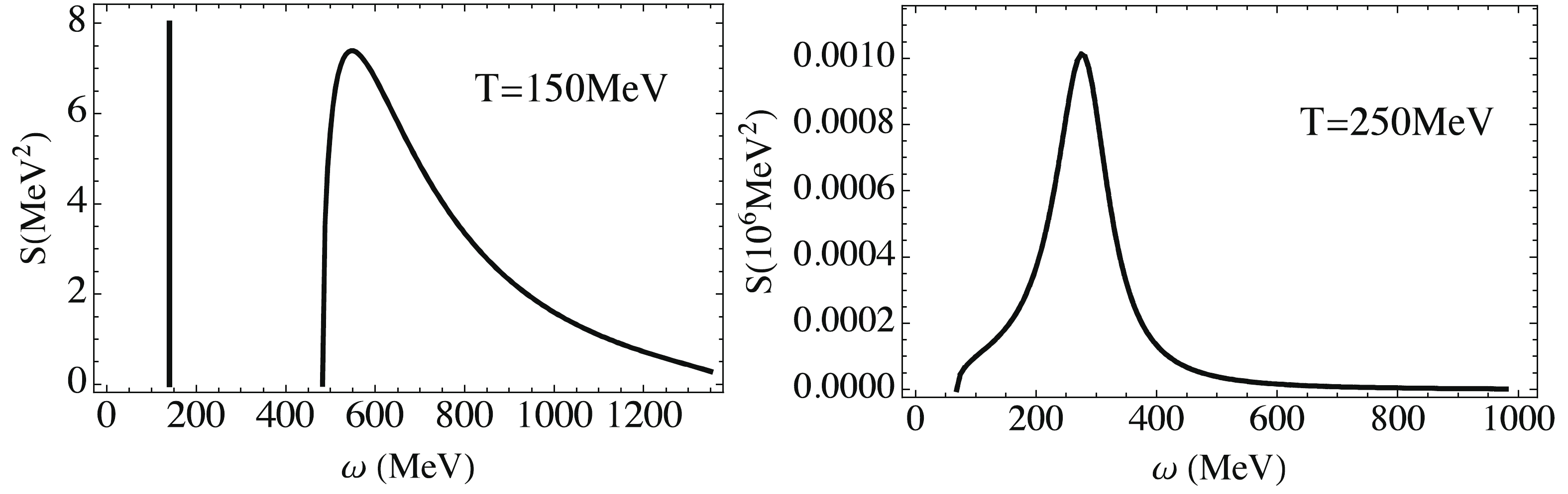
Figure 4. Dynamical structure factor
$ S(\omega,{ q}) $ at$ { q} = 0 $ for axial isospin density response ($ \hat{X} = \tau_3\gamma_5 $ ) below and above pion Mott transition temperature$ T_{\rm M} $ . We consider physical current quark mass$ m_0 = 5 $ MeV and$ \mu = 0 $ . The pion Mott transition temperature in this case is$ T_{\rm M} = 193 $ MeV. -
In the chiral limit (
$ m_0 = 0 $ ), the quarks become massless ($ M = 0 $ ) above the chiral phase transition temperature. In this case, we can show that$ C^\mu_{m}(Q) = 0 $ in the chiral symmetry restored phase. Therefore, the quasi-particle random phase approximation simply describes the linear response of a system of non-interacting massless quarks. However, it is generally expected that mesonic fluctuations play an important role above and near the chiral phase transition, indicating that the random phase approximation is inadequate for such a strongly interacting system. In this part, we consider a linear response theory beyond the random phase approximation. To this end, we recall that the generating functional in the Gaussian approximation can be expressed as$ \begin{array}{l} {\cal W}_{\rm NJL}[A] = {\cal W}_{\rm MF}[A]+{\cal W}_{\rm FL}[A]. \end{array} $

(118) In the previous random phase approximation, the meson-fluctuation contribution
$ {\cal W}_{\rm FL}[A] $ is neglected. We expect that this part becomes rather important near and above the chiral phase transition, where the quarks become massless and the mesonic degrees of freedom are still important. This is a general feature of a strongly interacting fermionic system. In strong-coupling superconductors, the pair fluctuation has an important contribution to the transport properties above and near the superconducting transition temperature [84,85].We consider the contribution from mesonic fluctuations. To derive the generating functional
$ {\cal W}_{\rm FL}[A] $ , we first note that$ \begin{array}{l} { G}_{\rm A}^{-1}(x,x^\prime) = {\cal G}_{A}^{-1}(x,x^\prime)-\Sigma_{\rm FL}(x,x^\prime), \end{array} $

(119) where
$ \Sigma_{\rm FL} $ includes mesonic fluctuation fields,$ \begin{array}{l} \Sigma_{\rm FL}(x,x^\prime) = \sum_{m = 0}^3\Gamma_{m}\phi_{m}(x)\delta(x-x^\prime), \end{array} $

(120) and
$ {\cal G}_{A}^{-1}(x,x^\prime) $ is the mean-field quark Green's function with the external source,$ \begin{array}{l} {\cal G}_{A}^{-1}(x,x^\prime) = {\cal G}^{-1}(x,x^\prime)-\Sigma_{\rm A}(x,x^\prime), \end{array} $

(121) with
$ {\cal G}^{-1}(x,x^\prime) $ and$ \Sigma_{A}(x,x^\prime) $ given in Eq. (79). Converting to the momentum space, we have$ \begin{split} { G}_{A}^{-1}(K,K^\prime) =& {\cal G}_{A}^{-1}(K,K^\prime)-\Sigma_{\rm FL}(K,K^\prime)\\ \Sigma_{\rm FL}(K,K^\prime) =& \sum_{m = 0}^3\Gamma_{m}\phi_{m}(K-K^\prime). \end{split} $

(122) Starting from Eqs. (67) and (68) and applying the derivative expansion, we obtain
$ \begin{split} {\cal S}_{\rm{eff}}^{(2)}[\sigma,{{\pi}}] = \frac{\beta V}{2}\sum\limits_{m,n = 0}^3\sum_{Q,Q^\prime}\phi_{m}(-Q)\left[{ D}_{\rm A}^{-1}(Q,Q^\prime)\right]\phi_{n}(Q^\prime), \end{split} $

(123) where
$ \begin{split} & \left[{ D}_{A}^{-1}(Q,Q^\prime)\right]_{mn} = \frac{\delta_{mn}}{2G}\delta_{Q,Q^\prime} \\&\quad +\frac{1}{\beta V}\sum\limits_{K,K^\prime}{\rm Tr}\left[{\cal G}_{A}(K,K^\prime-Q)\Gamma_{m}{\cal G}_{A}(K^\prime,K+Q^\prime)\Gamma_{n}\right]. \end{split} $

(124) Again, the path integral over the fluctuation fields
$ \phi_{m} $ can be calculated, and we obtain$ \begin{array}{l} {\cal W}_{\rm FL}[A] = \displaystyle\frac{1}{2}{\rm Tr}\ln[{ D}_{A}^{-1}(Q,Q^\prime)]. \end{array} $

(125) The trace here is also taken in the momentum space.
The next step is to expand
$ {\cal W}_{\rm FL}[A] $ in powers of the external source and induced perturbations. To this end, we first expand the inverse meson propagator$ { D}_{A}^{-1}(Q,Q^\prime) $ in powers of$ A_\mu $ and$ \eta_{m} $ . The expansion takes the form$ \begin{array}{l} { D}_{\rm A}^{-1}(Q,Q^\prime) = { D}^{-1}(Q)\delta_{Q,Q^\prime}+\Sigma^{(1)}(Q,Q^\prime)+\Sigma^{(2)}(Q,Q^\prime)+\cdots. \end{array} $

(126) Here,
$ { D}(Q) $ is the meson propagator evaluated in Sec. 3, and$ \Sigma^{(n)} $ denotes the nth-order expansion in$ A_\mu $ and$ \eta_{m} $ . In practice, we only need to evaluate the expansion up to the second order, since the higher order contributions are irrelevant to the linear response. Like$ { D}^{-1} $ ,$ \Sigma^{(1)} $ and$ \Sigma^{(2)} $ are$ 4\times4 $ matrices in the space spanned by$ {m} = 0,1,2,3 $ .To obtain
$ \Sigma^{(1)} $ and$ \Sigma^{(2)} $ , we note that in the momentum space, the inverse of the mean-field quark Green's function with external source,$ {\cal G}_{A}^{-1} $ , is given by$ \begin{array}{l} {\cal G}_{A}^{-1}(K,K^\prime) = {\cal G}^{-1}(K)\delta_{K,K^\prime}-\Sigma_{A}(K,K^\prime), \end{array} $

(127) where
$ \begin{split} \Sigma_{A}(K,K^\prime) = \sum\limits_{m = 0}^3\Gamma_{m}\eta_{m}(K-K^\prime)+\Gamma^\mu A_\mu(K-K^\prime). \end{split} $

(128) For convenience, here we express
$ \Sigma_{A} $ in a more compact form$ \begin{split} \Sigma_{A}(K,K^\prime) = \sum\limits_{i = 0}^7\tilde{\Gamma}^{i}\Phi_{i}(K-K^\prime), \end{split} $

(129) where
$ \tilde{\Gamma} $ is a compact notation of$ (\Gamma_{m},\Gamma^\mu) $ and$ \Phi $ is a compact form of$ (\eta_{m},A_\mu) $ . Here$ {i} = 0,1,2,3 $ still stands for$ \eta_{m} $ with$ {m} = 0,1,2,3 $ , and$ {i} = 4,5,6,7 $ stands for$ A_\mu $ with$ \mu = 0,1,2,3 $ . Applying the Taylor expansion for matrix functions, we obtain$ \begin{array}{l} {\cal G}_{A} = {\cal G}+{\cal G}\Sigma_{A}{\cal G}+{\cal G}\Sigma_{A}{\cal G}\Sigma_{A}{\cal G}+\cdots. \end{array} $

(130) This compact form of the Taylor expansion should be understood in all spaces. In the momentum space, we have explicitly
$ \begin{split} {\cal G}_{A}(K,K^\prime) =& {\cal G}(K,K^\prime)+\sum\limits_{K_1,K_2}{\cal G}(K,K_1)\Sigma_{A}(K_1,K_2){\cal G}(K_2,K^\prime)\\ &+\sum\limits_{K_1,K_2,K_3,K_4}{\cal G}(K,K_1)\Sigma_{A}(K_1,K_2){\cal G}(K_2,K_3)\\&\times\Sigma_{A}(K_3,K_4){\cal G}(K_4,K^\prime)+\cdots. \end{split} $

(131) According to the fact that
$ {\cal G}(K,K^\prime) = {\cal G}(K)\delta_{K,K^\prime} $ and$ \Sigma_{A}(K,K^\prime) = \Sigma_{A}(K-K^\prime) $ , this can be simplified to$ \begin{split} {\cal G}_{A}(K,K^\prime) =& {\cal G}(K)\delta_{K,K^\prime}+{\cal G}(K)\Sigma_{A}(K-K^\prime){\cal G}(K^\prime)\\ &+\sum\limits_{K^{\prime\prime}}{\cal G}(K)\Sigma_{A}(K-K^{\prime\prime}){\cal G}(K^{\prime\prime})\Sigma_{A}(K^{\prime\prime}-K^\prime)\\&\times{\cal G}(K^{\prime})+\cdots. \end{split} $

(132) The explicit form of
$ \Sigma^{(1)} $ and$ \Sigma^{(2)} $ can be derived by using the above expansion for$ {\cal G}_{A} $ .$ \Sigma^{(1)} $ is composed of one zeroth-order and one first-order contributions of$ {\cal G}_{A} $ . It is explicitly given by$ \begin{split} \Sigma^{(1)}_{mn}(Q,Q^\prime) = \sum\limits_{i = 0}^7{[X^{(1)}]}^{i}_{mn}(Q,Q^\prime)\Phi_{i}(Q-Q^\prime), \end{split} $

(133) where the coefficients are given by
$ \begin{split} {[X^{(1)}]}^{i}_{mn}(Q,Q^\prime) =& \frac{1}{\beta V}\sum\limits_K{\rm Tr}\left[{\cal G}(K)\Gamma_{m}{\cal G}(K\!+\!Q)\tilde{\Gamma}^{i} {\cal G}(K\!+\!Q^\prime)\Gamma_{n}\right]\\ &+\frac{1}{\beta V}\sum\limits_K{\rm Tr}\left[{\cal G}(K)\tilde{\Gamma}^{i}{\cal G}(K+Q^\prime-Q)\right.\\&\left.\times\Gamma_{m}{\cal G}(K+Q^\prime)\Gamma_{n}\right]. \end{split} $

(134) $ \Sigma^{(2)} $ includes two types of contributions. We have$ \begin{array}{l} \Sigma^{(2)} = \Sigma^{(2a)}+\Sigma^{(2b)}. \end{array} $

(135) $ \Sigma^{(2a)} $ is composed of one zeroth-order and one second-order contributions of$ {\cal G}_{A} $ . It is given by$ \begin{split} \Sigma^{(2a)}_{mn}(Q,Q^\prime) \!=\!& \frac{1}{\beta V}\sum\limits_{{i,j} = 0}^7\sum_{K,K^\prime}{[X^{(2a)}]}^{ij}_{mn}(Q,Q^\prime;K,K^\prime)\Phi_{i}(Q_1)\Phi_{j}(Q_2)\\& +\frac{1}{\beta V}\sum\limits_{{i,j} = 0}^7\sum_{K,K^\prime}{[Y^{(2a)}]}^{ij}_{mn}(Q,Q^\prime;K,K^\prime)\\&\times\Phi_{i}(Q_3)\Phi_{j}(Q_4). \end{split} $

(136) Here the momenta
$ Q_1,Q_2,Q_3 $ , and$ Q_4 $ are defined as$ \begin{array}{l} Q_1 = K-K^\prime+Q,\ \ \ \ \ \ Q_2 = K^\prime-K-Q^\prime,\\ Q_3 = K-K^\prime,\ \ \ \ \ \ Q_4 = K^\prime-K+Q-Q^\prime. \end{array} $

(137) The expansion coefficients are given by
$ \begin{split} {[X^{(2a)}]}^{ij}_{mn}(Q,Q^\prime;K,K^\prime) =& {\rm Tr}\left[{\cal G}(K)\Gamma_{m}{\cal G}(K+Q)\tilde{\Gamma}^{i}{\cal G}(K^\prime)\right.\\&\left.\times\tilde{\Gamma}^{j}{\cal G}(K+Q^\prime)\Gamma_{n}\right], \\ {[Y^{(2a)}]}^{ij}_{mn}(Q,Q^\prime;K,K^\prime) = &{\rm Tr}\left[{\cal G}(K)\tilde{\Gamma}^{i}{\cal G}(K^\prime)\tilde{\Gamma}^{j}{\cal G}(K+Q^\prime-Q)\right.\\&\left.\times \Gamma_{m}{\cal G}(K+Q^\prime)\Gamma_{n}\right]. \end{split} $

(138) $ \Sigma^{(2b)} $ is composed of two second-order contributions of$ {\cal G}_{A} $ . It reads$ \begin{split} \Sigma^{(2b)}_{mn}(Q,Q^\prime) =& \frac{1}{\beta V}\sum\limits_{{i,j} = 0}^7\sum_{K,K^\prime}{[X^{(2b)}]}^{ij}_{mn}\\&\times(Q,Q^\prime;K,K^\prime)\Phi_{i}(Q_1)\Phi_{j}(Q_2), \end{split} $

(139) where the expansion coefficient is given by
$ \begin{split} {[X^{(2b)}]}^{ij}_{mn}(Q,Q^\prime;K,K^\prime) =& {\rm Tr}\left[{\cal G}(K)\tilde{\Gamma}^{i}{\cal G}(K^\prime-Q)\right.\\&\times\left.\Gamma_{m}{\cal G}(K^\prime)\tilde{\Gamma}^{j}{\cal G}(K+Q^\prime)\Gamma_{n}\right]. \end{split} $

(140) -
Now we express the meson-fluctuation contribution to the generating functional as
$ \begin{split} {\cal W}_{\rm FL}[A;\eta] =& \frac{1}{2}{\rm Tr}\ln\left[{ D}^{-1}(Q)\delta_{Q,Q^\prime}+\Sigma^{(1)}(Q,Q^\prime)\right.\\&\left.+\Sigma^{(2a)}(Q,Q^\prime) +\Sigma^{(2b)}(Q,Q^\prime)+\cdots\right]. \end{split} $

(141) Here we start to demonstrate the explicit dependence on induced perturbations. Applying the trick of derivative expansion, we can expand
$ {\cal W}_{\rm FL} $ in powers of the external source as well as the induced perturbations. We have$ \begin{array}{l} {\cal W}_{\rm FL}[A;\eta] = {\cal W}_{\rm FL}^{(0)}+{\cal W}_{\rm FL}^{(1)}[A;\eta]+{\cal W}_{\rm FL}^{(2)}[A;\eta]+\cdots. \end{array} $

(142) It is evident that
$ {\cal W}_{\rm FL}^{(0)} = \beta V\Omega_{\rm FL} $ and hence the present linear response theory including the meson-fluctuation contribution is parallel to the meson-fluctuation theory of the equilibrium thermodynamics. The first-order expansion is given by$ \begin{split} {\cal W}_{\rm FL}^{(1)}[A;\eta] = \frac{1}{2}\sum\limits_{Q}{\rm Tr}_{4\rm D}\left[{ D}(Q)\Sigma^{(1)}(Q,Q)\right]. \end{split} $

(143) Here, the trace
$ {\rm Tr}_{4\rm D} $ is now taken only in the four-dimensional space spanned by$ {m},{n} = 0,1,2,3 $ . The second-order expansion can be expressed as$ \begin{array}{l} {\cal W}_{\rm FL}^{(2)}[A;\eta] = {\cal W}_{\rm FL}^{({\rm AL})}+{\cal W}_{\rm FL}^{({\rm SE})}+{\cal W}_{\rm FL}^{({\rm MT})}, \end{array} $

(144) where the three kinds of contributions are given by
$ \begin{split} {\cal W}_{\rm FL}^{({\rm AL})}[A;\eta] =& -\frac{1}{4}\sum\limits_{Q}\sum_{Q^\prime} {\rm Tr}_{4\rm D}\left[{ D}(Q)\Sigma^{(1)}(Q,Q^\prime)\right.\\&\times\left.{ D}(Q^\prime)\Sigma^{(1)}(Q^\prime,Q)\right],\\ {\cal W}_{\rm FL}^{({\rm SE})}[A;\eta] =& \frac{1}{2}\sum\limits_{Q}{\rm Tr}_{4\rm D}\left[{ D}(Q)\Sigma^{(2a)}(Q,Q)\right],\\ {\cal W}_{\rm FL}^{({\rm MT})}[A;\eta] =& \frac{1}{2}\sum\limits_{Q}{\rm Tr}_{4\rm D}\left[{ D}(Q)\Sigma^{(2b)}(Q,Q)\right], \end{split} $

(145) which correspond diagrammatically to the Aslamazov-Lakin (AL), self-energy (SE) or density-of-state, and Maki-Thompson (MT) contributions.
To obtain the response functions, we need to eliminate the induced perturbations
$ \eta_{m}(Q) $ . Noting that the present theory of linear response is a natural generalization of the meson-fluctuation theory of the equilibrium thermodynamics, where the order parameter is determined at the mean-field level, we determine the induced perturbations$ \eta_{m}(Q) $ still by minimizing the mean-field generation functional, i.e.,$ \begin{split} \frac{\delta{\cal W}_{\rm MF}^{(2)}[A;\eta]}{\delta \eta_{m}(Q)} = 0, \end{split} $

(146) which leads to
$ \begin{split} \eta_{m}(Q) =& -\frac{C^\mu_{m}(-Q)}{\displaystyle\frac{1}{2G}+\Pi_{m}(Q)}A_\mu(Q)+O(A^2),\\ \eta_{m}(-Q) =& -\frac{C^\mu_{m}(Q)}{\displaystyle\frac{1}{2G}+\Pi_{m}(Q)}A_\mu(-Q)+O(A^2). \end{split} $

(147) Later, we will show that the use of the above relations is also crucial to recover the correct number susceptibility in the static and long-wavelength limit.
-
Unlike the mean-field theory or random phase approximation, the first-order contribution, Eq. (143), becomes highly nontrivial. It can be expressed as
$ \begin{split} {\cal W}_{\rm FL}^{(1)}[A;\eta] = \beta V\sum\limits_{{i} = 1}^7{\cal C}_{i}\Phi_{i}(0), \end{split} $

(148) where the coefficients read
$ \begin{split} {\cal C}_{i} = \frac{1}{2\beta V}\sum_{Q}{\rm Tr}_{4\rm D}\left\{{ D}(Q)[X^{(1)}]^{i}(Q,Q)\right\}. \end{split} $

(149) Using the explicit expression of
$ X^{(1)} $ , we can show that possible nonvanishing coefficients are$ \begin{split} {\cal C}_0 = \frac{\partial \Omega_{\rm FL}(M,\mu_{X})}{\partial M}, \ \ \ \ \ \ \ {\cal C}_4 = \frac{\partial \Omega_{\rm FL}(M,\mu_{X})}{\partial\mu_{X}}. \end{split} $

(150) Since we consider only nonzero baryon chemical potential, here the effective chemical potential
$ \mu_{X} = A_0(0) $ is nonvanishing only for the vector current case$ (\hat{X} = 1) $ . Thus,$ {\cal C}_4 $ is nonvanishing only for the case$ \hat{X} = 1 $ , where$ \mu_{X} $ corresponds to the quark chemical potential$ \mu $ . The fact that$ {\cal C}_0\neq0 $ indicates that the first-order contribution$ {\cal W}_{\rm FL}^{(1)}[A;\eta] $ cannot be simply neglected, since it does contribute to the linear response. To understand this, we note that when eliminating the induced perturbation$ \eta_0(0) $ , Eq. (147) is not adequate. Actually, the contributions of the order$ O(A^2) $ in Eq. (147) become important. To obtain these contributions, we should expand the mean-field generating functional$ {\cal W}_{\rm MF}[A;\eta] $ up to the third order in A and$ \eta $ . We have$ \begin{split} {\cal W}_{\rm MF}^{(3)}[A;\eta] =& \frac{1}{3}\sum\limits_{K}\sum_{K^\prime}\sum_{K^{\prime\prime}}{\rm Tr}\left[{\cal G}(K)\Sigma_{A}(K,K^\prime){\cal G}(K^\prime)\right. \\&\times\left.\Sigma_{A}(K^\prime,K^{\prime\prime}) {\cal G}(K^{\prime\prime})\Sigma_{A}(K^{\prime\prime},K)\right]. \end{split} $

(151) By defining
$ K^\prime = K+Q $ and$ K^{\prime\prime} = K+Q^\prime $ , we obtain$ \begin{split} \frac{{\cal W}_{\rm MF}^{(3)}[A;\eta]}{\beta V} =& \frac{1}{3}\sum\limits_{{i,j,k} = 0}^7\sum_{Q}\sum_{Q^\prime}F_{ijk}(Q,Q^\prime)\\&\times \Phi_{i}(-Q)\Phi_{j}(Q-Q^\prime)\Phi_{k}(Q^\prime), \end{split} $

(152) where the function
$ F_{ijk}(Q,Q^\prime) $ is defined as$ \begin{split} F_{ijk}(Q,Q^\prime) = \frac{1}{\beta V}\sum\limits_{K}{\rm Tr}\left[{\cal G}(K)\tilde{\Gamma}^{i}{\cal G}(K+Q)\tilde{\Gamma}^{j}{\cal G}(K+Q^\prime)\tilde{\Gamma}^{k}\right]. \end{split} $

(153) Using the extreme condition
$ \begin{split} \frac{\delta{\cal W}_{\rm MF}[A;\eta]}{\delta\eta_{0}(Q)} = 0 \end{split} $

(154) with
$ {\cal W}_{\rm MF} = {\cal W}_{\rm MF}^{(0)}+{\cal W}_{\rm MF}^{(1)}+{\cal W}_{\rm MF}^{(2)}+{\cal W}_{\rm MF}^{(3)}+\cdots $ , we obtain$ \begin{split} \eta_0(0) = {\cal R}_1A_0(0)+\frac{1}{2}\sum\limits_{{i,j} = 0}^7 \sum_Q{\cal U}_{ij}(Q)\Phi_{i}(-Q)\Phi_{j}(Q)+\cdots, \end{split} $

(155) where the coefficients
$ {\cal R}_1 $ and$ {\cal U}_{ij}(Q) $ are given by$ \begin{split} {\cal R}_1 =& -\lim_{Q\rightarrow0}\frac{C^0_0(-Q)}{\displaystyle\frac{1}{2G}+\Pi_0(Q)},\\ {\cal U}_{ij}(Q) = &\frac{2}{3}\lim_{Q^\prime\rightarrow0}\frac{F_{0{ij}}(-Q^\prime,Q)+F_{{i}0{j}}(Q+Q^\prime,Q)+F_{{ij}0}(Q,Q^\prime)}{\displaystyle\frac{1}{2G}+\Pi_0(Q)}. \end{split} $

(156) Here the the static and long-wavelength limit of an arbitrary function
$ {\cal A}(Q) $ should be understood as$\lim_{Q\rightarrow0} $ $ {\cal A}(Q) = \lim_{{ q}\rightarrow0}{\cal A}(iq_l = 0,{ q}) $ . For the purpose of linear response, we apply Eq. (147) and obtain$ \begin{array}{l} \eta_0(0) = {\cal R}_1A_0(0)+\displaystyle\frac{1}{2} \sum\limits_Q{\cal R}_2^{\mu\nu}(Q)A_{\mu}(-Q)A_{\nu}(Q)+O(A^3). \end{array} $

(157) Here, the explicit form of the function
$ {\cal R}_2^{\mu\nu}(Q) $ is not shown. It is evident that$ \begin{split} {\cal R}_1 = \frac{\partial M(\mu_{X})}{\partial \mu_{X}}, \ \ \ \ \ \ \lim_{Q\rightarrow0}{\cal R}_2^{00}(Q) = \frac{\partial^2 M(\mu_{X})}{\partial \mu_{X}^2}. \end{split} $

(158) Substituting the expansion (155) into Eq. (148), we eliminate the induced perturbations and obtain
$ \begin{split} \frac{{\cal W}_{\rm FL}^{(1)}[A]}{\beta V} =& - (n_{X})_{\rm FL}A_0(0)\\&+\frac{1}{2} \sum\limits_Q\Pi_{\rm OP}^{\mu\nu}(Q)A_{\mu}(-Q)A_{\nu}(Q)+\cdots, \end{split} $

(159) where
$ (n_{X})_{\rm FL} $ is the fluctuation contribution to the charge density,$ \begin{split} (n_{X})_{\rm FL} = -\frac{\partial \Omega_{\rm FL}(M,\mu_{X})}{\partial\mu_{X}}-\frac{\partial \Omega_{\rm FL}(M,\mu_{X})}{\partial M}\frac{\partial M(\mu_{X})}{\partial \mu_{X}}. \end{split} $

(160) The first-order term
$ {\cal W}_{\rm FL}^{(1)} $ thus yields a nontrivial contribution to the response function, which is given by$ \begin{array}{l} \Pi_{\rm OP}^{\mu\nu}(Q) = {\cal C}_0{\cal R}_2^{\mu\nu}(Q). \end{array} $

(161) It is evident that this contribution is due to the non-vanishing chiral condensate. In the chiral limit, this contribution vanishes above the phase transition temperature, where
$ {\cal C}_0 = 0 $ . Therefore, we denote it as the order parameter induced (OP) contribution, which can be expressed as$ \begin{split} {\cal W}_{\rm FL}^{({\rm OP})}[A] = \frac{\beta V}{2}\sum\limits_Q\Pi_{\rm OP}^{\mu\nu}(Q)A_{\mu}(-Q)A_{\nu}(Q). \end{split} $

(162) -
The Aslamazov-Lakin contribution is given by
$ \begin{split} {\cal W}_{\rm FL}^{({\rm AL})}[A;\eta] =& -\frac{1}{4}\sum\limits_{Q} \sum_{Q^\prime}{\rm Tr}_{\rm 4D} \left[{ D}(Q)\Sigma^{(1)}(Q,Q^\prime)\right.\\&\left.\times{ D}(Q^\prime)\Sigma^{(1)}(Q^\prime,Q)\right]. \end{split} $

(163) After some manipulation, it can be expressed as
$ \begin{split} {\cal W}_{\rm FL}^{({\rm AL})}[A;\eta] = \frac{\beta V}{2}\sum\limits_{{i,j} = 0}^7\sum_{Q} \Xi_{ij}^{\rm AL}(Q)\Phi_{i}(-Q)\Phi_{j}(Q), \end{split} $

(164) where the function
$ \Xi_{ij}^{\rm AL}(Q) $ is given by$ \begin{split} \Xi_{ij}^{\rm AL}(Q) =& -\frac{1}{2}\frac{1}{\beta V}\sum_{P}{\rm Tr}_{\rm 4D} \left\{{ D}(P)[X^{(1)}]^{i}(P,P+Q)\right.\\&\left.\times{ D}(P+Q)[X^{(1)}]^{j}(P+Q,P)\right\}. \end{split} $

(165) Here the matrices
$ [X^{(1)}]^{i}(P,P+Q) $ and$ [X^{(1)}]^{j}(P+Q,P) $ are defined as$ \begin{split} [X^{(1)}]^{i}_{mn}(P,P+Q) =& \frac{1}{\beta V}\sum\limits_K{\rm Tr} \left[{\cal G}(K)\Gamma_{m}{\cal G}(K+P)\right.\\&\times\left.\tilde{\Gamma}^{i} {\cal G}(K+P+Q)\Gamma_{n}\right]\\ &+\frac{1}{\beta V}\sum\limits_K{\rm Tr}\left[{\cal G}(K)\tilde{\Gamma}^{i}{\cal G}(K+Q)\right.\\ &\left.\times\Gamma_{m}{\cal G}(K+P+Q)\Gamma_{n}\right],\\ {[X^{(1)}]}^{j}_{mn}(P+Q,P) =& \frac{1}{\beta V}\sum\limits_K{\rm Tr}\left[{\cal G}(K)\Gamma_{m}{\cal G}(K+P+Q)\right.\\&\left.\times\tilde{\Gamma}^{j} {\cal G}(K+P)\Gamma_{n}\right]\\ &+\frac{1}{\beta V}\sum\limits_K{\rm Tr}\left[{\cal G}(K)\tilde{\Gamma}^{j}{\cal G}(K-Q)\right.\\&\left.\times\Gamma_{m}{\cal G}(K+P)\Gamma_{n}\right]. \end{split} $

(166) We finally use Eq. (147) to eliminate the induced perturbations and obtain the AL contribution
$ \begin{split} {\cal W}_{\rm FL}^{({\rm AL})}[A] = \frac{\beta V}{2}\sum\limits_{Q} \Pi_{\rm AL}^{\mu\nu}(Q)A_{\mu}(-Q)A_{\nu}(Q), \end{split} $

(167) where
$ \Pi_{\rm AL}^{\mu\nu}(Q) $ is the AL contribution to the response function. -
The self-energy or density-of-state contribution is given by
$ \begin{split} {\cal W}_{\rm FL}^{({\rm SE})}[A;\eta] = \frac{1}{2}\sum\limits_{Q}{\rm Tr}_{\rm 4D}\left[{ D}(Q)\Sigma^{(2a)}(Q,Q)\right], \end{split} $

(168) After some manipulations, it can be expressed as
$ \begin{split} {\cal W}_{\rm FL}^{({\rm SE})}[A;\eta] = \frac{\beta V}{2}\sum\limits_{{i,j} = 1}^8\sum_{Q}\Xi_{ij}^{\rm SE}(Q)\Phi_{i}(-Q)\Phi_{j}(Q), \end{split} $

(169) where the function
$ \Xi_{ij}^{\rm SE}(Q) $ is given by$ \begin{split} \Xi_{ij}^{\rm SE}(Q) =& \frac{1}{\beta V}\sum\limits_{P}{\rm Tr}_{4\rm D}\left[{ D}(P){ Y}^{ij}(P,Q)\right] \\&+\frac{1}{\beta V}\sum\limits_{P}{\rm Tr}_{\rm 4D}\left[{ D}(P){ Z}^{ij}(P,Q)\right]. \end{split} $

(170) Here the matrices
$ { Y}^{ij}(P,Q) $ and$ { Z}^{ij}(P,Q) $ are defined as$ \begin{split} { Y}^{ij}_{mn}(P,Q) =& \frac{1}{\beta V}\sum\limits_{K}{\rm Tr}\left[{\cal G}(K-P)\Gamma_{m}{\cal G}(K)\right.\\&\times\left.\tilde{\Gamma}^{i}{\cal G}(K+Q)\tilde{\Gamma}^{j}{\cal G}(K)\Gamma_{n}\right],\\ { Z}^{ij}_{mn}(P,Q) =& \frac{1}{\beta V}\sum_{K}{\rm Tr}\left[{\cal G}(K)\tilde{\Gamma}^{i}{\cal G}(K+Q)\right.\\&\left.\times\tilde{\Gamma}^{j}{\cal G}(K) \Gamma_{m}{\cal G}(K+P)\Gamma_{n}\right]. \end{split} $

(171) We finally use Eq. (147) to eliminate the induced perturbations and obtain the SE contribution
$ \begin{split} {\cal W}_{\rm FL}^{({\rm SE})}[A] = \frac{\beta V}{2}\sum\limits_{Q} \Pi_{\rm SE}^{\mu\nu}(Q)A_{\mu}(-Q)A_{\nu}(Q), \end{split} $

(172) where
$ \Pi_{\rm SE}^{\mu\nu}(Q) $ is the SE contribution to the response function. -
The Maki-Thompson contribution is given by
$ \begin{split} {\cal W}_{\rm FL}^{({\rm MT})}[A;\eta] = \frac{1}{2}\sum\limits_{Q}{\rm Tr}_{4\rm D}\left[{ D}(Q)\Sigma^{(2b)}(Q,Q)\right]. \end{split} $

(173) After some manipulation, it can be expressed as
$ \begin{split} {\cal W}_{\rm FL}^{({\rm MT})}[A;\eta] = \frac{1}{2}\sum\limits_{{i,j} = 1}^8\sum_{Q}\Xi_{ij}^{\rm MT}(Q)\Phi_{i}(-Q)\Phi_{j}(Q), \end{split} $

(174) where the function
$ \Xi_{ij}^{\rm MT}(Q) $ is given by$ \begin{split} \Xi_{ij}^{\rm MT}(Q) = \frac{1}{\beta V}\sum\limits_{P}{\rm Tr}_{4\rm D}\left[{ D}(P){ W}^{ij}(P,Q)\right]. \end{split} $

(175) Here the matrix
$ { W}^{ij}(P,Q) $ is defined as$ \begin{split} { W}^{ij}(P,Q) =& \frac{1}{\beta V}\sum\limits_{K}{\rm Tr} \left[{\cal G}(K)\tilde{\Gamma}^{i}{\cal G}(K+Q)\right.\\&\left.\times\Gamma_{m}{\cal G}(K+P+Q)\tilde{\Gamma}^{j}{\cal G}(K+P)\Gamma_{n}\right]. \end{split} $

(176) We finally use Eq. (147) to eliminate the induced perturbations and obtain the MT contribution
$ \begin{split} {\cal W}_{\rm FL}^{({\rm MT})}[A] = \frac{\beta V}{2}\sum\limits_{Q} \Pi_{\rm MT}^{\mu\nu}(Q)A_{\mu}(-Q)A_{\nu}(Q), \end{split} $

(177) where
$ \Pi_{\rm MT}^{\mu\nu}(Q) $ is the MT contribution to the response function.Combining all contributions, the meson-fluctuation contribution to the linear response is given by
$ \begin{split} {\cal W}_{\rm FL}^{(2)}[A] = \frac{1}{2}\sum\limits_{Q}\Pi_{\rm FL}^{\mu\nu}(Q)A_{\mu}(-Q)A_{\nu}(Q), \end{split} $

(178) where
$ \Pi_{\rm FL}^{\mu\nu}(Q) $ is a summation of all the above contributions,$ \begin{array}{l} \Pi_{\rm FL}^{\mu\nu}(Q) = \Pi_{\rm OP}^{\mu\nu}(Q)+\Pi_{\rm AL}^{\mu\nu}(Q)+\Pi_{\rm SE}^{\mu\nu}(Q)+\Pi_{\rm MT}^{\mu\nu}(Q). \end{array} $

(179) Summarizing the mean-field and the meson-fluctuation contributions, we have
$ \begin{split} {\cal W}_{\rm NJL}^{(2)}[A] = \frac{1}{2}\sum\limits_{Q}\Pi^{\mu\nu}(Q)A_{\mu}(-Q)A_{\nu}(Q), \end{split} $

(180) where the full response function within the present theory is given by
$ \begin{array}{l} \Pi^{\mu\nu}(Q) = \Pi_{\rm MF}^{\mu\nu}(Q)+\Pi_{\rm FL}^{\mu\nu}(Q). \end{array} $

(181) -
Now, we verify the static and long-wavelength limit of the above linear response theory. In this limit, it is obvious that the density response function
$ \Pi^{00}(Q\rightarrow0) $ should recover the charge susceptibility$ \kappa_{X} $ associated with the channel X, i.e.,$ \begin{split} \Pi^{00}(Q\rightarrow0) = -\kappa_{X} = \frac{\partial^2\Omega(T,\mu_{X})}{\partial \mu_{X}^2}. \end{split} $

(182) In condensed matter theory, this is the so-called compressibility sum rule [75]. Here, we emphasize that the correct static and long-wavelength limit of an arbitrary function
$ {\cal A}(Q) $ should be understood as$ \begin{array}{l} {\cal A}(Q\rightarrow0) = \lim_{{ q}\rightarrow0}{\cal A}(iq_l = 0,{ q}). \end{array} $

(183) In the mean-field theory, the thermodynamic potential is given by
$ \Omega_{\rm MF}(\mu_{X},M) $ , where the dependence on the temperature is not explicitly shown. Note that the effective quark mass M is also an implicit function of$ \mu_{X} $ ,$ M = M(\mu_{X}) $ , which should be determined by the mean-field gap equation$ \begin{split} \frac{\partial \Omega_{\rm MF}(\mu_{X},M)}{\partial M} = 0. \end{split} $

(184) The charge susceptibility can be evaluated as
$ \begin{split} (\kappa_{X})_{\rm MF} =& -\frac{\partial^2\Omega_{\rm MF}(\mu_{X},M)}{\partial \mu_{X}^2}\\&-\frac{\partial^2\Omega_{\rm MF}(\mu_{X},M)}{\partial \mu_{X}\partial M} \frac{\partial M(\mu_{X})}{\partial\mu_{X}}. \end{split} $

(185) The quantity
$ \partial M/\partial\mu_{X} $ can be deduced from the gap equation. We have$ \begin{split} \frac{\partial^2\Omega_{\rm MF}(\mu_{X},M)}{\partial \mu_{X} \partial M }+\frac{\partial^2\Omega_{\rm MF}(\mu_{X},M)}{\partial M^2} \frac{\partial M(\mu_{X})}{\partial\mu_{X}} = 0, \end{split} $

(186) which leads to
$ \begin{split} \frac{\partial M(\mu_{X})}{\partial\mu_{X}} = -\frac{\partial^2\Omega_{\rm MF}(\mu_{X},M)}{\partial \mu_{X} \partial M }\left[\frac{\partial^2\Omega_{\rm MF}(\mu_{X},M)}{\partial M^2}\right]^{-1}. \end{split} $

(187) Hence we obtain
$ \begin{split} (\kappa_{X})_{\rm MF} =& -\frac{\partial^2\Omega_{\rm MF}(\mu_{X},M)}{\partial \mu_{X}^2}\\&+\left[\frac{\partial^2\Omega_{\rm MF}(\mu_{X},M)}{\partial \mu_{X}\partial M}\right]^2 \left[\frac{\partial^2\Omega_{\rm MF}(\mu_{X},M)}{\partial M^2}\right]^{-1}. \end{split} $

(188) In contrast, from the linear response theory, we have
$ \begin{split} \Pi_{\rm MF}^{00}(Q) = \Pi_{ b}^{00}(Q)-\sum\limits_{m = 0}^3\frac{C^0_{m}(Q)C^0_{m}(-Q)}{\dfrac{1}{2G}+\Pi_{m}(Q)}. \end{split} $

(189) In the static and long-wavelength limit
$ Q\rightarrow0 $ , we have$ C^0_{m}(Q)\rightarrow0 $ for$ {m} = 1,2,3 $ . Thus, we obtain$ \begin{split} \Pi_{\rm MF}^{00}(Q\rightarrow 0) =& \Pi_{b}^{00}(Q\rightarrow 0)\\&-\frac{\left[C^0_0(Q\rightarrow 0)\right]^2}{\dfrac{1}{2G}+\Pi_{0}(Q\rightarrow0)}. \end{split} $

(190) Using the explicit form of the above functions, we can show that
$ \begin{split} \Pi_{b}^{00}(Q\rightarrow0) =& \frac{\partial^2\Omega_{\rm MF}(\mu_{X},M)}{\partial \mu_{X}^2},\\ C^0_0(Q\rightarrow0) =& \frac{\partial^2\Omega_{\rm MF}(\mu_{X},M)}{\partial \mu_{X} \partial M },\\ \frac{1}{2G}+\Pi_{0}(Q\rightarrow0) =& \frac{\partial^2\Omega_{\rm MF}(\mu_{X},M)}{\partial M^2}. \end{split} $

(191) Thus, the compressibility sum rule is satisfied in the mean-field theory, i.e.,
$ \begin{array}{l} \Pi_{\rm MF}^{00}(Q\rightarrow0) = -(\kappa_{X})_{\rm MF}. \end{array} $

(192) When the meson fluctuations are taken into account, we have
$ \begin{array}{l} \kappa_{X} = (\kappa_{X})_{\rm MF}+(\kappa_{X})_{\rm FL}, \end{array} $

(193) where the meson-fluctuation contribution can be evaluated as
$ \begin{split} (\kappa_{X})_{\rm FL} =& -\frac{\partial^2\Omega_{\rm FL}(\mu_{X},M)}{\partial \mu_{X}^2}-2\frac{\partial^2\Omega_{\rm FL}(\mu_{X},M)}{\partial \mu_{X}\partial M} \frac{\partial M(\mu_{X})}{\partial\mu_{X}}\\&-\!\frac{\partial^2\Omega_{\rm FL}(\mu_{X},M)}{\partial M^2}\!\left[\!\frac{\partial M(\mu_{X})}{\partial\mu_{X}}\!\right]^2\!-\!\frac{\partial\Omega_{\rm FL}(\mu_{X},M)}{\partial M}\frac{\partial^2\! M(\mu_{X})}{\partial\mu_{X}^2}. \end{split} $

(194) We note that the effective quark mass
$ M(\mu_{X}) $ is still determined by the mean-field gap equation. On the other hand, the meson-fluctuation contribution to the density response function can be decomposed as$ \begin{array}{l} \Pi_{\rm FL}^{00}(Q) = \Pi_{\rm OP}^{00}(Q)+\Pi_{\rm AL}^{00}(Q)+\Pi_{\rm SE}^{00}(Q)+\Pi_{\rm MT}^{00}(Q). \end{array} $

(195) We can show that the first three terms in
$ (\kappa_{X})_{\rm FL} $ are related to the sum of AL, SE, and MT contributions in the$ Q\rightarrow0 $ limit,$ \begin{split} \lim_{Q\rightarrow0}&\left[\Pi_{\rm AL}^{00}(Q)+\Pi_{\rm SE}^{00}(Q)+\Pi_{\rm MT}^{00}(Q)\right]\\ =& \frac{\partial^2\Omega_{\rm FL}(\mu_{X},M)}{\partial \mu_{X}^2}+2\frac{\partial^2\Omega_{\rm FL}(\mu_{X},M)}{\partial \mu_{X}\partial M} \frac{\partial M(\mu_{X})}{\partial\mu_{X}}\\&+\frac{\partial^2\Omega_{\rm FL}(\mu_{X},M)}{\partial M^2}\left[\frac{\partial M(\mu_{X})}{\partial\mu_{X}}\right]^2. \end{split} $

(196) To prove this, we recall that in the presence of only
$ A_0(Q) $ , the induced perturbations are given by$ \begin{split} \eta_{m}(Q) =& -\frac{C^0_{m}(-Q)A_0(Q)}{\displaystyle\frac{1}{2G}+\Pi_{m}(Q)}+O(A^2),\\ \eta_{m}(-Q) =& -\frac{C^0_{m}(Q)A_0(-Q)}{\displaystyle\frac{1}{2G}+\Pi_{m}(Q)}+O(A^2). \end{split} $

(197) In the limit
$ Q\rightarrow0 $ , only$ \eta_{0} $ survives and hence$ \begin{split} \lim_{Q\rightarrow0}\frac{\eta_0(Q)}{A_0(Q)} = -\lim_{Q\rightarrow0}\frac{C^0_0(-Q)}{\displaystyle\frac{1}{2G}+\Pi_0(Q)} = \frac{\partial M(\mu_{X})}{\partial\mu_{X}}. \end{split} $

(198) The order parameter induced contribution,
$ \Pi_{\rm OP}^{00}(Q) $ , is related to the last term in$ (\kappa_{X})_{\rm FL} $ . We have$ \begin{array}{l} \Pi_{\rm OP}^{00}(Q\rightarrow0) = {\cal C}_0{\cal R}_2^{00}(Q\rightarrow 0). \end{array} $

(199) Using the fact that
$ \begin{split} {\cal C}_0 = \frac{\partial\Omega_{\rm FL}(\mu_{X},M)}{\partial M}, \ \ \ \ \ \ \lim_{Q\rightarrow0}{\cal R}_2^{00}(Q) = \frac{\partial^2 M(\mu_{X})}{\partial \mu_{X}^2}, \end{split} $

(200) we find that the the last term in
$ (\kappa_{X})_{\rm FL} $ is exactly given by the OP contribution. We can further understand this result by working out the explicit form$ \begin{split} \frac{\partial^2 M(\mu_{X})}{\partial \mu_{X}^2} =& - \left\{\frac{\partial^3\Omega_{\rm MF}(\mu_{X},M)}{\partial \mu_{X}^2\partial M}+2\frac{\partial^3\Omega_{\rm MF}(\mu_{X},M)}{\partial \mu_{X}\partial M^2} \frac{\partial M(\mu_{X})}{\partial\mu_{X}}\right.\\&\left.+\frac{\partial^3\Omega_{\rm MF}(\mu_{X},M)}{\partial M^3}\left[\frac{\partial M(\mu_{X})}{\partial\mu_{X}}\right]^2\right\}\\& \times\left[\frac{\partial^2\Omega_{\rm MF}(\mu_{X},M)}{\partial M^2}\right]^{-1}. \end{split} $

(201) In summary, we have shown that the compressibility sum rule is exactly satisfied in the linear response theory including the meson fluctuations. The order parameter induced contribution is rather crucial to recover the correct static and long-wavelength limit.
-
One special case we are interested in is the chiral symmetry restored phase (
$ T>T_c $ ) in the chiral limit ($ m_0 = 0 $ ). In this case, we have$ {\cal C}_0 = 0 $ , and hence the order parameter induced contribution vanishes. Also, we have$ C_{m}^\mu(Q) = 0 $ , indicating that we do not need to consider the induced perturbations$ \eta_{m}(Q) $ . In this case, the formalism becomes rather simple and we can identify various contributions diagrammatically.In the chiral symmetry restored phase, the sigma meson and pions become degenerate. We have
$ \begin{array}{l} [{ D}(Q)]_{mn} = {\cal D}(Q)\delta_{mn} , \end{array} $

(202) where the propagator of the mesonic modes above
$ T_c $ is given by$ \begin{split} {\cal D}^{-1}(Q) =& \frac{1}{2G}+N_cN_f \int{{\rm d}^3{ k}\over (2\pi)^3}\Bigg[\left(\frac{1-f(E_{ k}^+)-f(E_{{ k}+{ q}}^-)}{iq_l-E_{ k}-E_{{ k}+{ q}}}\right.\\&\left.-\frac{1-f(E_{ k}^-)-f(E_{{ k}+{ q}}^+)}{iq_l+E_{ k}+E_{{ k}+{ q}}}\right) \left(1+\frac{{ k}\cdot ({ k+ q})}{E_{ k} E_{{ k}+{ q}}}\right)\\ &+\left(\frac{f(E_{ k}^-)-f(E_{{ k}+{ q}}^-)}{iq_l+E_{ k}-E_{{ k}+{ q}}}-\frac{f(E_{ k}^+)-f(E_{{ k}+{ q}}^+)}{iq_l-E_{ k}+E_{{ k}+{ q}}}\right)\\&\times \left(1-\frac{{ k}\cdot ({ k+ q})}{E_{ k} E_{{ k}+{ q}}}\right)\Bigg]. \end{split} $

(203) Here
$ E_{ k} = |{ k}| $ for$ T>T_c $ . Due to the degeneracy of the sigma meson and pions, various contributions to the linear response above$ T_c $ become simple. -
Above
$ T_c $ , the Aslamazov-Lakin contribution is given by$ \begin{split} {\cal W}_{\rm FL}^{({\rm AL})} = \frac{\beta V}{2}\sum\limits_{Q} \Pi_{\rm AL}^{\mu\nu}(Q)A_{\mu}(-Q)A_{\nu}(Q), \end{split} $

(204) where the AL response function
$ \Pi_{\rm AL}^{\mu\nu}(Q) $ is given by$ \begin{split} \Pi_{\rm AL}^{\mu\nu}(Q) = -\frac{2}{\beta V}\sum\limits_{P}\left[{\cal D}(P){\cal D}(P+Q){\cal X}^\mu(P,Q){\cal X}^\nu(-P,-Q)\right]. \end{split} $

(205) The function
$ {\cal X}^\mu(P,Q) $ here is defined as$ \begin{split} {\cal X}^\mu(P,Q) =& \frac{1}{\beta V}\sum\limits_K{\rm Tr} \left[{\cal G}(K)\Gamma^{\mu}{\cal G}(K+Q){\cal G}(K-P)\right]\\ &+\frac{1}{\beta V}\sum_K{\rm Tr}\left[{\cal G}(K-Q)\Gamma^{\mu}{\cal G}(K){\cal G}(K+P)\right]. \end{split} $

(206) Here, the quark propagator
$ {\cal G}(K) $ is given in Eq. (85) with$ M = 0 $ . The AL contribution can be diagrammatically demonstrated in Fig. 5.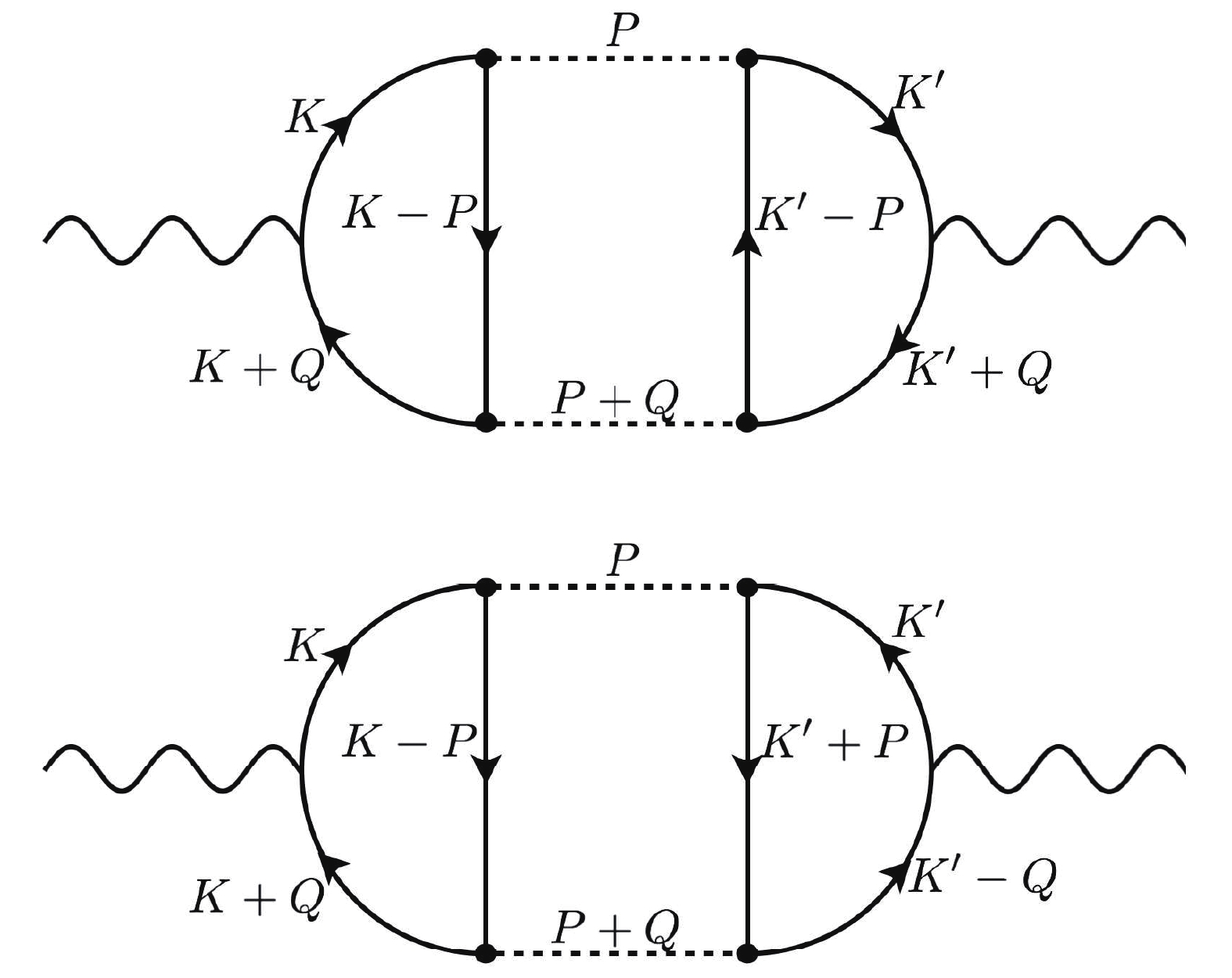
Figure 5. Diagrammatic representation of Aslamazov-Lakin contribution. Note that there are two kinds of AL-type diagrams. The solid lines with arrows denote the quark propagator, the dashed lines depict the meson propagator, and wavy lines represent the external source.
-
Above
$ T_c $ , the self-energy or density-of-state contribution is given by$ \begin{split} {\cal W}_{\rm FL}^{({\rm SE})} = \frac{\beta V}{2}\sum\limits_{Q} \Pi_{\rm SE}^{\mu\nu}(Q)A_{\mu}(-Q)A_{\nu}(Q), \end{split} $

(207) where the SE response function
$ \Pi_{\rm SE}^{\mu\nu}(Q) $ is given by$ \begin{split} \Pi_{\rm SE}^{\mu\nu}(Q) = \frac{8}{\beta V}\sum\limits_{P}\left[{\cal D}(P){\cal Y}^{\mu\nu}(P,Q)\right]. \end{split} $

(208) Here, the function
$ {\cal Y}^{\mu\nu}(P,Q) $ is explicitly given by$ \begin{split} {\cal Y}^{\mu\nu}(P,Q) = \frac{1}{\beta V}\sum\limits_{K}{\rm Tr}\left[{\cal G}(K)\Gamma^{\mu}{\cal G}(K+Q)\Gamma^{\nu}{\cal G}(K){\cal G}(K+P)\right]. \end{split} $

(209) Note that
$ \Pi_{\rm SE}^{\mu\nu}(Q) $ can also be written as$ \begin{split} \Pi_{\rm SE}^{\mu\nu}(Q) = \frac{2}{\beta V}\sum\limits_{K}{\rm Tr}\left[\Gamma^{\mu}{\cal G}(K+Q)\Gamma^{\nu}{\cal G}(K)\Sigma_{q}(K){\cal G}(K)\right], \end{split} $

(210) where
$ \Sigma_{q} $ is the quark self-energy,$ \begin{split} \Sigma_{q}(K) = \frac{4}{\beta V}\sum\limits_{P}\left[{\cal D}(P){\cal G}(K+P)\right]. \end{split} $

(211) The SE contribution is diagrammatically illustrated in Fig. 6.
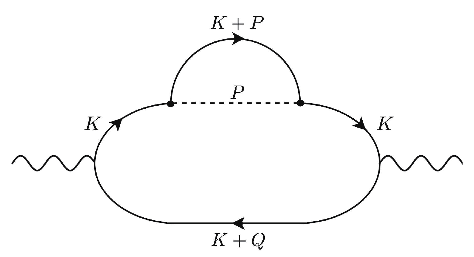
Figure 6. Diagrammatic representation of the self-energy contribution. Notations are the same as in Fig. 5.
-
Above
$ T_c $ , the Maki-Thompson contribution is given by$ \begin{split} {\cal W}_{\rm FL}^{({\rm MT})} = \frac{\beta V}{2}\sum\limits_{Q} \Pi_{\rm MT}^{\mu\nu}(Q)A_{\mu}(-Q)A_{\nu}(Q), \end{split} $

(212) where the MT response function
$ \Pi_{\rm MT}^{\mu\nu}(Q) $ is given by$ \begin{split} \Pi_{\rm MT}^{\mu\nu}(Q) = \frac{4}{\beta V}\sum\limits_{P}\left[{\cal D}(P){\cal W}^{\mu\nu}(P,Q)\right]. \end{split} $

(213) Here, the function
$ {\cal W}^{\mu\nu}(P,Q) $ is explicitly given by$ \begin{split} {\cal W}^{\mu\nu}(P,Q) =& \frac{1}{\beta V}\sum\limits_{K}{\rm Tr} \left[{\cal G}(K)\Gamma^{\mu}{\cal G}(K+Q)\right.\\&\times\left.{\cal G}(K+P+Q)\Gamma^{\nu}{\cal G}(K+P)\right]. \end{split} $

(214) The MT contribution is diagrammatically illustrated in Fig. 7.
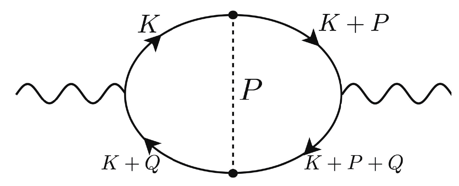
Figure 7. Diagrammatic representation of the Maki-Thompson contribution. Notations are the same as in Fig. 5.
In summary, the AL, SE, and MT contributions can be diagrammatically identified in the chiral symmetry restored phase. These contributions include the propagator of the degenerate mesonic modes,
$ {\cal {D}}(Q) $ . Near the chiral phase transition temperature, these mesonic modes are soft modes and are nearly massless. Therefore, we expect that these mesonic modes have a significant effect on the transport properties near the transition. -
In this work, we studied the linear response of hot and dense matter in the two-flavor Nambu-Jona-Lasino model. The linear response theory is formulated within the path integral approach. In this elegant formalism, the current-current correlation functions or response functions are conveniently calculated by introducing the conjugated external gauge field as an external source and expanding the generating functional in powers of the external source. Parallel to the well-established approximations for the equilibrium thermodynamics, we studied the linear response within the mean-field theory and beyond-mean-field theory, taking into account mesonic contributions.
In the mean-field approximation, the response function recovers the quasiparticle random phase approximation. The dynamical structure factors for various density responses have been studied using this approximation. In the long-wavelength limit, the dynamical structure factors are nonzero only for the axial baryon density and the axial isospin density channels. For the axial isospin density channel, the dynamical structure factor can be used to reveal the Mott dissociation of pions at finite temperature. Below the Mott transition temperature, the dynamical structure factor reveals a pole plus continuum structure. Above the Mott transition temperature, it only has a continuum part.
It is generally expected that the mesonic degrees of freedom are important both in the chiral symmetry broken and restored phases. However, in the chiral symmetry restored phase, the random phase approximation describes the linear response of a hot and dense gas of non-interacting massless quarks. Therefore, the mesonic degrees of freedom are not taken into account above and near the chiral phase transition temperature. In this study, we have developed a linear response theory based on the meson-fluctuation theory, which properly includes the mesonic degrees of freedom. The mesonic fluctuations naturally give rise to three kinds of famous diagrammatic contributions: the Aslamazov-Lakin contribution, the self-energy or density-of-state contribution, and the Maki-Thompson contribution. In the chiral symmetry breaking phase, we also found an additional chiral order parameter induced contribution, which ensures that the temporal component of the response functions in the static and long-wavelength limit recovers the correct charge susceptibility defined using the equilibrium thermodynamic quantities. These contributions from the mesonic fluctuations are expected to have significant effects on the transport properties of hot and dense matter around the chiral phase transition or crossover, where mesonic degrees of freedom are still important.
Response functions of hot and dense matter in the Nambu-Jona-Lasino model
- Received Date: 2019-04-10
- Accepted Date: 2019-06-09
- Available Online: 2019-09-01
Abstract: We investigate current-current correlation functions, or the so-called response functions of a two-flavor Nambu-Jona-Lasino model at finite temperature and density. The linear response is investigated introducing the conjugated gauge fields as external sources within the functional path integral approach. The response functions can be obtained by expanding the generational functional in powers of the external sources. We derive the response functions parallel to two well-established approximations for equilibrium thermodynamics, namely mean-field theory and a beyond-mean-field theory, taking into account mesonic contributions. Response functions based on the mean-field theory recover the so-called quasiparticle random phase approximation. We calculate the dynamical structure factors for the density responses in various channels within the random phase approximation, showing that the dynamical structure factors in the baryon axial vector and isospin axial vector channels can be used to reveal the quark mass gap and the Mott dissociation of mesons, respectively. Noting that the mesonic contributions are not taken into account in the random phase approximation, we also derive the response functions parallel to the beyond-mean-field theory. We show that the mesonic fluctuations naturally give rise to three kinds of famous diagrammatic contributions: the Aslamazov-Lakin contribution, the self-energy or density-of-state contribution, and the Maki-Thompson contribution. Unlike the equilibrium case, in evaluating the fluctuation contributions, we need to carefully treat the linear terms in external sources and the induced perturbations. In the chiral symmetry breaking phase, we find an additional chiral order parameter induced contribution, which ensures that the temporal component of the response functions in the static and long-wavelength limit recovers the correct charge susceptibility defined using the equilibrium thermodynamic quantities. These contributions from mesonic fluctuations are expected to have significant effects on the transport properties of hot and dense matter around the chiral phase transition or crossover, where the mesonic degrees of freedom are still important.


 DownLoad: