A close look at the competition of isovector and isoscalar pairing in A=18 and 20 even-even N≈Z nuclei

It is generally recognized that, like the well studied isovector ($ T = 1 $, $ J = 0 $) pairing, the isoscalar ($ T = 0 $, $ J = 1 $) pairing should also be of importance for the ground state of ${N} \approx { Z} $ nuclei. There are a number of investigations of this problem with the Bardeen-Cooper-Schrieffer and Hartree-Fock-Bogolyubov approximations [1]. Shell model calculations with effective interactions focusing on the neutron-proton pairing correlations have also been carried out [2]. For example, the pair correlation was investigated by means of the Shell Model Monte Carlo (SMMC) method performed with the modified Kuo-Brown interaction (KB3) and the pairing plus quadrupole-quadrupole (PQQ) interaction in the fp-shell [3-6]. Direct diagonalization of the KB3 interaction in the fp-shell showed that the strength of the isovector pairing interaction seems 2-3 times stronger than the isoscalar strength when the total isospin is small [7,8]. Shell model calculations based on effective interactions with respect to the isovector and isoscalar pairing were also performed in fp, sdfp, and $ f_{5}pg_{9} $ subspaces [9-11]. Systematic analysis of $ { N} \approx { Z} $ nuclei in various model spaces with the extended pairing plus the quadrupole-quadrupole (EPQQ) Hamiltonian has been carried out extensively [12-29]. Very recently, a distinct quartet structure has also been proposed and applied to the isovector ($ T = 1 $, $ J = 0 $) and isoscalar ($ T = 0 $, $ J = 1 $) pairing correlations [30-32], which showed that the $ J = 0 $ quartet plays a leading role in the structure of the ground state of $ ds $-shell nuclei. The isovector and isoscalar pairing in $ N = Z $ nuclei was also systematically studied by analyzing the shell model wave functions with effective interactions [33,34]. Although the agreement of the shell model results with the experiments suggests that the isovector and isoscalar pairing interactions are realistic, the actual interaction strengths are subject to considerable uncertainty due to the fact that the competition of isovector and isoscalar pairing, deformation, and other correlations leads to a very complex picture.

In this work, inspired by the afore mentioned investigations, we examine the competition of isovector and isoscalar pairing in A=18 and 20 even-even ${ N} \approx { Z} $ nuclei described by the mean-field plus quadrupole-quadrupole (QQ), pairing and particle-hole interactions, which is diagonalized in the basis ${ U}(24) \supset ({ U}(6)\supset {{SU}}(3)\supset {{SO}}(3)) \otimes $$ ({ U}(4)\supset{ {SU}}_S(2)\otimes {{SU}}_T(2)) $ in the $ L = 0 $ configuration subspace. Due to its simplicity and explicitness, we are able to take a close look at the competition of isovector and isoscalar pairing in the presence of deformation and particle-hole interactions, the latter of which has not been considered directly in the estimates of the pairing interactions.

The Hamiltonian of the spherical mean-field plus dynamic QQ, pairing, and particle-hole model is given by

where $ \hat{n}_{j} = \sum_{m_{j}\,m_{t}}a^{†}_{jm_{j};tm_{t}}a_{jm_{j};tm_{t}} $ is the number operator of valence nucleons in the $ j $-orbit, $ m_{j} $ is the quantum number of the projection of the total angular momentum of valence nucleons in the orbit, $ \epsilon_{j} $ is the corresponding single-particle energy given by the spherical shell model, $ t = 1/2 $ and $ m_{t} $ are the quantum numbers of the isospin and of its projection, respectively, $ \chi>0 $ is the dynamic QQ interaction strength, $ \hat{Q}_{\mu} $ is the Elliott dynamic quadrupole operator [35,36], with which the quadrupole-quadrupole interaction, $ -\chi\,\hat{Q}\cdot\hat{Q} $, is spin and isospin independent. The pairing interaction term $ \hat{H}_{\rm {P}} $ in (1) is given as

where $ G_{\rm {V}} $ and $ G_{\rm {S}} $ are the strengths of the isovector and isoscalar pairing interactions,

with the orbital angular momentum $ L = 0 $, spin $ S = 0 $, and isospin $ T = 1 $, and

with $ L = 0 $, $ S = 1 $, and $ T = 0 $. The particle-hole interaction $ \hat{H}_{\rm {ph}} $ in (1) is given by

where $ \hat{n} = \sum_{j}\hat{n}_{j} $ is the total number operator of valence nucleons, $ {\cal F}^{011}_{0\,\mu\nu} $ are the particle-hole (Gamow-Teller) operators, which are generators of the U(4) group with $ L = 0 $ and $ S = T = 1 $, and $ \mu $ and $ \nu $ stand for the quantum numbers of the spin and isospin projections, respectively. The Hamiltonian (1) with only the pairing part was studied in the O(8) basis previously [37-40]. The first term in the particle-hole interaction (5) was introduced in [41,42] and also adopted in [43]. Here, the second term of (5) is introduced to ensure that the matrix elements of (5) are only related to the second order invariant (Casimir operator) of U(4), spin and isospin in the ${ U}(24) \supset { U}(6) \otimes { U}(4)$ basis, the expression for which will be shown later. Moreover, the shell model Hamiltonian with the QQ interaction and the spin and isospin independent $ L = 0 $ pairing interaction in the $ ds $-shell was studied in [44,45].

For simplicity, the analysis is restricted to the $ ds $-shell, and the spin-orbit splitting in the shell model mean-field is neglected. Hence, the first term in (1) becomes a constant for a given nucleus. It is obvious that the Hamiltonian (1), neglecting the spin-orbit splitting in the shell model mean-field, commutes with the total particle number, spin, isospin, and the total angular momentum operators. For this case, it is convenient to use the valance nucleon creation operators in the LST-coupling scheme with $ \{a^{\text †}_{lm_{l};\; sm_{s};\; tm_{t}}\} $, where $ l = 0,\,2 $, $ s = 1/2 $ and $ t = 1/2 $ are the orbital angular momentum, spin, and isospin of the valence nucleon, respectively. It is well known that the particle-number preserving bilinear operators $ \{a^{\text †}_{lm_{l};\; sm_{s}\,tm_{t}}a_{l'm'_{l};\; sm'_{s}\,tm'_{t}}\} $ generate the unitary group U($ {\cal N} $4), where $ {\cal N} = \sum_{l}(2l+1) $. Thus, $ {\cal N} = 6 $ for the $ ds $-shell, and $ {\cal N} = 10 $ for the fp-shell, and so on. Since a $ k $-particle state must be totally anti-symmetric with respect to any permutation among the $ k $ particles, only totally anti-symmetric irreducible representation (irrep) $ [1^{k}] $ of U($ {\cal N} $4) is allowed, where $ [1^{k}] $ may be represented by the corresponding Young diagram with $ k $ boxes. For our purpose, we adopt a complete set of basis vectors for irrep $ [1^{k}] $ of U(24) in the U(24)$\supset \left({ U}(6)\supset { SU}(3)\supset { SO(3)}\right)\otimes $$ \left( { U}(4)\supset { SU}_{S}(2)\otimes { SU}_{T}(2)\right) $, which is denoted as $ \vert k\,\alpha (LS) $$JM_{J};\,T M_{T}\rangle\equiv \vert [1^{k}][\tilde{f}][f]\,\beta(\lambda\mu)\kappa L;\rho\, S TM_{T}\,JM_{J}\rangle $, where $ k $ is the total number of particles, $ \alpha $ stands for the set of quantum numbers $ [f] $, $ (\lambda\mu) $, $ \beta $, $ \rho $, and $ \kappa $ involved, $ f_{1} $, $ f_{2} $, $ f_{3} $, $ f_{4} $ in the four-rowed irrep $ [f] $ of U(4) satisfy $ \sum_{i}f_{i} = k $, $ \rho $ and $ \beta $ are the branching multiplicity labels needed in the reductions U(24) $ \downarrow $ U(6)$ \otimes $U$ _{ST} $(4) and U(6) $ \downarrow $ SU(3), respectively, $ (\lambda\mu) $ is an allowed irrep of SU(3), $ L $, $ S $, $ J $, $ M_{J} $, and T, $ M_{T} $ are quantum numbers of the orbital angular momentum, spin, total angular momentum, its projection, and of the isospin and its projection, respectively. The branching rule of $ [1^{k}] $ in the reduction $ { U}({\cal N}4)\downarrow $${ U}({\cal N}) \otimes { U}(4) $ is branching multiplicity-free and given by [40, 44-46]

where $ [\tilde{f}] $ is the irrep of U(6), which is the conjugated Young diagram of $ [f_{1},f_{2},f_{3},f_{4}] $. In the calculation, the elementary isoscalar factors (Wigner coefficients), also called one-particle coefficients of fractional parentage (CFPs) of $ { U}({\cal N}4)\supset { U}({\cal N})\otimes { U}(4) $ , are needed. As shown in [46], the $ { U}({\cal NM})\supset { U}({\cal N})\otimes { U}({\cal M}) $ Isoscalar Factors (ISFs) are related to the relevant CG coefficients of the symmetric groups. For a totally antisymmetric irrep of $ { U}({\cal N}{\cal M}) $, the elementary ISF can be expressed as [46]

where $ [\sigma] $ or $ [\sigma'] $ labels the irrep of $ { U}({\cal N}) $, $ [\nu] $ or $ [\nu'] $ labels that of $ U({\cal M}) $, $ [\tilde{\nu}] $ stands for the conjugated Young diagram of $ [\nu] $, and $ h_{[\sigma']} $ or $ h_{[\sigma]} $ is the dimension of the irrep $ [\sigma'] $ or $ [\sigma] $ of the symmetric group $ S_{k} $ or $ S_{k+1} $. It is obvious that ISF shown in (7) is independent of $ {\cal N} $ and $ {\cal M} $, and only depends on the irreps of $ {\rm U}({\cal N}) $ or $ {\rm U}({\cal M}) $ involved. Using the Robinson dimension formula of the symmetric groups [47], we have

with which the elementary ISFs of $ { U}({\cal N} 4)\supset { U}({\cal N})\otimes { U}(4) $ are explicitly known. The elementary ISFs $ \left\langle\begin{array}{l} \; \; \; \; \; \; {[\tilde{f^{\prime}}]}\cr \beta^{\prime}(\lambda^{\prime},\mu^{\prime})\\ \end{array} \begin{array}{l} \; \; [1]\cr (20)\\ \end{array}\right. \left| \begin{array}{l} \; \; \; \; {[\tilde{f}]}\cr {\beta (\lambda ,\mu )}\\ \end{array}\right\rangle $ of $ { U}(6)\supset { SU}(3) $ needed for the $ ds $-shell were given by Akiyama [48]. In the calculation, we use the Draayer-Akiyama code for the Wigner coefficients $ \left\langle\begin{array}{l} \; (\lambda\mu)\; (20)\cr \; \; \kappa\, L\; \; \; \; \; \; l\cr \end{array}\right. \left\vert\begin{array}{l} (\lambda^{\prime}\mu^{\prime})\cr \; \kappa^{\prime}\, L^{\prime}\cr \end{array}\right\rangle $ of $ { SU}(3)\supset{ SO}(3) $ described in [49,50]. Finally, ISFs of $ { U}(4)\supset { SU}_{S}(2)\otimes $$ { SU}_{T}(2) $ $ \left\langle\begin{array}{l} \; \; [f]\; \; \; [1]\cr \rho\,S\,T\; \; s\,t\cr \end{array}\right. \left\vert\begin{array}{l} \; \; [f^{\prime}]\cr \rho^{\prime}\, S^{\prime}\, T^{\prime}\cr \end{array}\right\rangle $ given in [46,51] are adopted.

Thus, the matrix elements of $ \hat{H}_{\rm P,V} $ and those of $ \hat{H}_{\rm P,S} $ in the U(24) basis are given by

in which

where the curly braces denote the related 6j-symbol. In these matrix elements, the one-particle reduced matrix elements $ \langle k'\,\alpha' LST||a^{\text †}_{lst}||k\,{\alpha}{L}{S}{T}\rangle $ in the basis $ {\rm U}(24)\supset \left({\rm U}(6)\supset\right.$$\left. { SU}(3)\supset { SO}(3)\right)\otimes\left( { U}(4)_{ST}\supset { SU}_{S}(2)\otimes { SU}_{T}(2)\right) $ are the most important, which can be expressed, according to the Racah factorization lemma, as

where $ \langle [1^{k^{\prime}}]||a^{\text †}||[1^{k}]\rangle = \sqrt{k+1}\,\delta_{k^{\prime}\, k+1} $ is the U(24) reduced matrix element. Moreover, the QQ and particle-hole interaction terms in (1) only contribute to the diagonal matrix elements of the Hamiltonian (1) in the U(24) basis with

for the corresponding SU(3) irrep $ (\lambda\,\mu) $ and

for the corresponding U(4) irrep $ [f_{1},f_2, f_3, f_4] $, where the first term in the parentheses on the right-hand-side of (13) is the eigenvalue of the second order Casimir operator of U(4). Once the matrix elements of (1) are thus obtained, the eigenstates of (1) can be expressed as

where $ C^{(\zeta)}_{\alpha} $ is the $ \alpha $-component of the $ \zeta $-th eigenvector of (1) after diagonalization in the U(24) basis.

In order to analyze the competition of isovector and isoscalar pairing in the presence of other interactions, we take $ k = 2 $ and $ k = 4 $ cases corresponding to A = 18 and A = 20 even-even systems. In the analysis, only the $ L = 0 $ basis vectors are taken in the diagonalization, which should be a good approximation to a few lowest $ J = 0 $, $ J = 1 $ and $ T\leqslant 2 $ levels with the number of U(24) basis vectors greatly reduced. We set $ \chi = 1-y $, $ G_{\rm {V}} = y(1+x) $, and $ G_{\rm {S}} = y(1-x) $ in (1) with $ 0\leqslant y\leqslant 1 $ MeV and $ -1\leqslant x\leqslant 1 $, where the units of $ \chi $ and $ y $ are MeV, which is reasonable for the A = 18 and 20 systems.

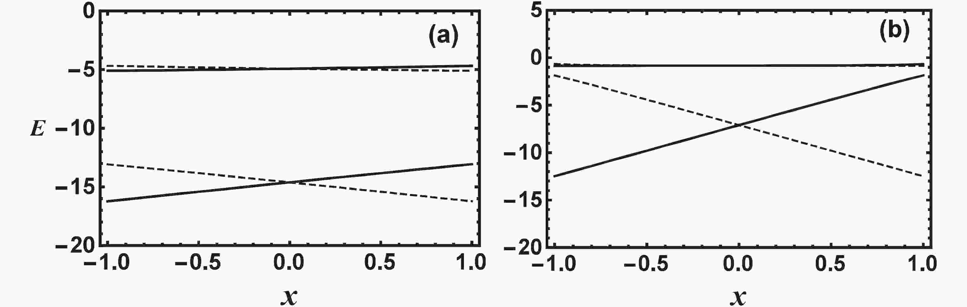
For the $ k = 2 $ case, only ($ T = 0 $, $ S = 1 $) or ($ T = 1 $, $ S = 0 $) states in $ [2,0]\otimes [1,1] $ irrep of U(6)$ \otimes $U(4) are allowed with $ L = 0 $, which is consistent with the fact that these are indeed the only possible states in the low energy region in A = 18 even-even nuclei, especially in $ ^{18}{\rm{F}} $. In this case, the particle-hole interaction term becomes a constant with no influence on the competition of isovector and isoscalar pairing. Since there are only two SU(3) irreps with $ (\lambda\mu) = (0\,2) $ and $ (4\,0) $ involved, there are four ($ T = 0 $, $ S = 1 $) and ($ T = 1 $, $ S = 0 $) states in total. Figure 1 shows the ($ T = 0 $, $ S = 1 $) levels (solid line) and the ($ T = 1 $, $ S = 0 $) levels (dashed line) with $ y = 0.3 $ and $ y = 0.9 $ MeV, respectively. It can be seen that there is a crossing of the ($ T = 0 $, $ S = 1 $) level with ($ T = 1 $, $ S = 0 $) . The crossing point with $ x = 0 $ corresponds to the U(4) symmetry point. Therefore, whether the ground state is ($ T = 0 $, $ S = 1 $) or ($ T = 1 $, $ S = 0 $), it is driven mainly by the competition of isovector and isoscalar pairing. Since the ground state of $ ^{18}{\rm{F}} $ is in this case $ T = 0 $ and $ S = 1 $ , the isoscalar pairing strength $ G_{\rm {S}} $ should always be a little larger $ G_{\rm {V}} $. On the other hand, the system deformation represented by the QQ interaction greatly alters the energy gaps between ($ T = 0 $, $ S = 1 $) and ($ T = 1 $, $ S = 0 $) and the other excited levels. Comparing panels (a) and (b) in Fig. 1, it is clearly seen that for stronger QQ interaction, the energy gap between the lowest ($ T = 0 $, $ S = 1 $) and ($ T = 1 $, $ S = 0 $) levels becomes smaller, while the energy gaps between the lowest two levels and the other two excited levels become larger.

Figure 1.  ($ T = 0 $, $ S = 1 $) level (solid lines) and ($ T = 1 $, $ S = 0 $) level (dashed lines) as function of $ x $ for two different QQ strengths in the $ k = 2 $ system, where the excitation energy $ E $ is in MeV The contribution of the constant mean-field and the particle-hole interaction to the total energy of the system is not included. The particle-hole interaction is in this case irrelevant for the excitation energy. Panel (a) is for $ \chi = 0.7 $ MeV, and panel (b) is for $ \chi = 0.1 $ MeV.

For the $ k = 4 $ case, the low-lying spectrum, even for the $ S = 0 $ and $ S = 1 $ levels, becomes complicated. In particular, the particle-hole interaction is now effective in the spectrum. In this case, the low-lying $ S = 0 $ or $ S = 1 $ levels are associated with $ T = 0,\,1,\,2 $, which is only possible for $ ^{20}{\rm{Ne}} $. Since $ T\geqslant 1 $ should be satisfied in $ ^{20}{\rm{F}} $ and $ ^{20}{\rm{Na}} $, $ T = 0 $ levels, shown in Fig. 2 , are removed for these two cases. Similarly, there are only $ T = 2 $ levels in $ ^{20}{\rm{O}} $ and $ ^{20}{\rm{Mg}} $, for which the isoscalar pairing interaction is ineffective for the ($ T = 2 $, $ S = 0 $) levels with $ L = 0 $. The isoscalar pairing interaction is effective only for $ S = 1 $ levels when $ T = 2 $, which have $ L\neq 0 $ , and is not considered here. Specifically, when only the $ L = 0 $ configuration is considered, the ($ T = 0 $, $ S = 0 $) states are in $ [4]\otimes[1,1,1,1] $ and $ [2,2]\otimes [2,2] $ irreps, ($ T = 1 $, $ S = 0 $) or ($ T = 0 $, $ S = 1 $) states are in $ [2,0]\otimes[1,1] $ and $ [3,1]\otimes [2,1,1] $ irreps, and ($ T = 2 $, $ S = 0 $) states are in $ [2,2]\otimes[2,2] $ irrep of U(6)$ \otimes $U(4), respectively.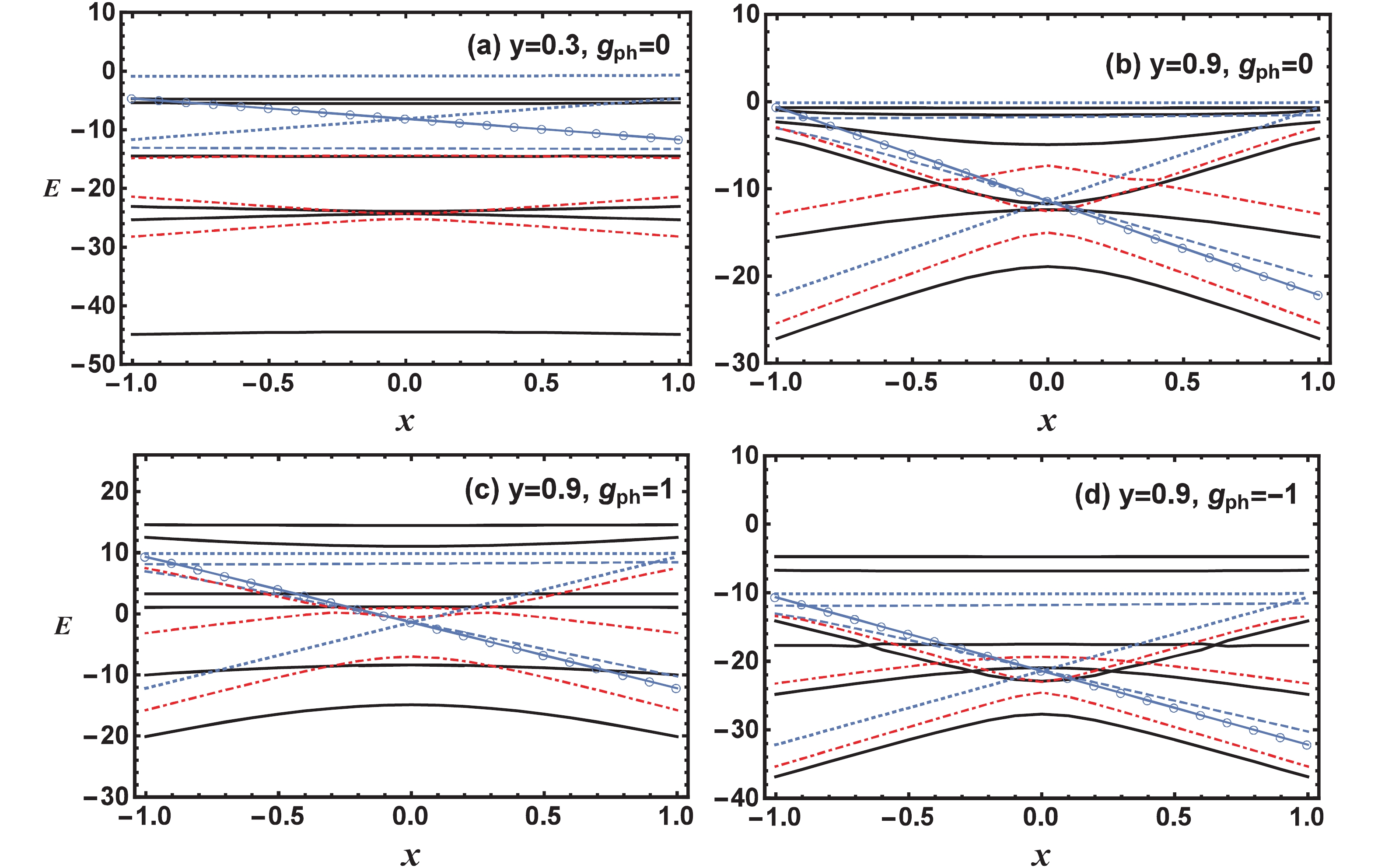

Figure 2.  (color online) ($ T = 0 $, $ S = 0 $) levels (solid lines), ($ T = 1 $, $ S = 1 $) levels (red dot-dashed lines), the lowest ($ T = 1 $, $ S = 0 $) levels (line-connected open circles), ($ T = 0 $, $ S = 1 $) levels (dotted lines), and ($ T = 2 $, $ S = 0 $) levels (dashed lines) as function of x for two different QQ and particle-hole interaction strengths in the $ k = 4 $ sysem. The excitation energy E and the parameters y and $ g_{\rm {ph}} $ are in MeV. The contribution of the constant mean-field energy to the total energy of the system is not included.

As shown in Fig. 2, if the QQ interaction strength is strong enough, as shown in panel (a), the ground state always has $ T = 0 $ and $ S = 0 $, and there is a large energy gap between the lowest ($ T = 0 $, $ S = 0 $) and the other excited levels. If the QQ interaction strength is weak, as shown in panel (b) of Fig. 2, the ground state is still the lowest ($ T = 0 $, $ S = 0 $) state among the relatively high density of levels, where the U(4) point with $ x = 0 $ corresponds to the highest density. Furthermore, when the particle-hole interaction is switched on, the energy gap between the ground state and the excited levels becomes larger if the particle-hole interaction is repulsive, while the gap becomes smaller if the particle-hole interaction is attractive.

Since the matrix elements of the particle-hole interaction shown in (13) are linear in $ T(T+1) $, it may be related to the Wigner term in the binding energy [52]. However, whether the particle-hole interaction contributes to the binding energy is mainly determined by the sign of $ g_{\rm {ph}} $. When $ g_{\rm {ph}}>0 $, the particle-hole interaction is always repulsive, which reduces the binding energy, but the contribution decreases with increasing T. When $ g_{\rm {ph}}<0 $, the particle-hole interaction increases the binding energy, but again the contribution decreases with increasing T. Nevertheless, it is observed that a larger value of $ g_{\rm {ph}} $ is needed to fit the excitation energies of a nucleus if its ground state isospin T is small. With increasing ground state isospin T of the neighboring nucleus, the value of $ g_{\rm {ph}} $ of the neighboring nucleus decreases, where $ g_{\rm {ph}}<0 $ for the ground state of a nucleus with the largest T, as is indeed shown for the A = 18 and 20 nuclei. Therefore, although the mechanism of the particle-hole contribution to the binding energy is different, and not always proportional to $ T(T+1) $ like in the Wigner energy term in the binding energy formula [52], it is indeed indirectly related to the Wigner term.

To estimate the strengths of the the isovector and isoscalar pairing interactions in A = 18 and 20 even-even N$ \approx $Z nuclei, not only the excited levels but also the total contribution to the binding energy should be properly considered in order to reduce the arbitrariness in choosing the model parameters. Since the valence particles are confined to the $ ds $-shell, $ ^{16}{\rm{O}} $ is taken as the inert core. Thus, the binding energy of a nucleus is defined as

where

with $ I = \vert N-Z\vert/A $, are the surface, Coulomb, and symmetry energy [53], respectively, $ N_{\pi} $ and $ N_{\nu} $ are the number of valence protons and neutrons, respectively, $ E_{0} $ is the average binding energy per valence nucleon in the ds-shell, which is almost a constant contribution of the shell model mean-field, and $ E^{(1)}_{k} $ with $ k = N_{\pi}+N_{\nu} $ is the $ k $-particle ground state energy determined by the model Hamiltonian (1). The I correction term, introduced in the symmetry energy in (16), approximately describes the Wigner effect [53], which is checked against the symmetry energy with the Wigner effect given in [52]. Therefore, if the parameters of the model Hamiltonian are properly adjusted, the $ k $-particle ground state energy with fixed $ k = N_{\pi}+N_{\nu} $ for $ N_{\pi}\geq0 $ and $ N_{\nu}\geq0 $ should satisfy

where $ \Delta B(N_{\pi},N_{\nu}) $ is determined by (15). This provides a reasonable constraint for fitting the $ k $-particle ground state energy $ E^{(1)}_{k} $ of the model Hamiltonian (1), and is used in the fit. However, if $ g_{\rm {ph}} $ is used as a free parameter, which is required for fitting the low-lying levels of A = 20 nuclei, there is still arbitrariness in choosing $ g_{\rm {ph}} $ for the A = 18 nuclei, because the excited energy levels concerned are independent of $ g_{\rm {ph}} $. Therefore, the isovector and isoscalar pairing strengths for A = 18 nuclei are estimated from the related excited levels only, so that the parameter $ g_{\rm {ph}} $ for each nucleus is estimated according to (17). For A = 20 nuclei, both the excited levels and the total contribution to the binding energy are considered in the estimate of the isovector and isoscalar pairing strengths.

Since the model is restricted to the $ L = 0 $ configuration subspace, only a few lowest $ J = 0 $ and $ J = 1 $ levels can be roughly fitted by using (1) to estimate the isovector and isoscalar pairing strengths in each nucleus. We only focus on a best fit to the experimental data for each nucleus, for which the systematics of the model parameters is not applied. The total ground state energy of a nucleus (17) may be expressed as $ E_{k}^{(1)} = E_{\rm QQ}+E_{\rm {P}}+E_{\rm {ph}} $, where $ E_{\rm QQ} $, $ E_{\rm {P}} $, and $ E_{\rm {ph}} $ are the mean values of the ground state energy contribution from the QQ interaction, pairing interaction, and particle-hole interaction, respectively. The QQ interaction strength may be estimated by $ \chi_{\rm {rot}}\sim (E_{2^{+}_{1}}-E_{0^{+}_{\rm{1}}})/6 $ related to the moment of inertia of the ground band, where $ E_{2^{+}_{1}} $ and $ E_{0^{+}_{\rm{1}}} = E_{k}^{(1)} $ are the excitation energy of the first $ 2^+ $ state and the ground state energy of a nucleus, respectively, for which the energy levels in the ground band are assumed to be rotational. Since the level spectra of these nuclei are not typically rotational, it is found that the actual QQ interaction strength $ \chi $ should be taken smaller than that determined from the moment of inertia of the ground band with $ \chi<\chi_{\rm {rot}} $. Otherwise, due to the fact that $ E_{k}^{(1)} $ is a constant, the pairing contribution $ E_{\rm {P}} $ would be too small to generate appropriate energy gaps of the low-lying levels if $ \chi $ is too large when the total contribution to the binding with the constraint (17) is applied. In the fits, $ \chi = 0.245 $ MeV for $ ^{18}{\rm{O}} $ and $ ^{18}{\rm{Ne}} $, and $ \chi = 0.066 $ MeV for $ ^{18}{\rm{F}} $, which are $ 70 $% of the values determined by the moment of inertia of the ground band. Similarly, $ \chi = 0.095 $ MeV for $ ^{20}{\rm{O}} $ and $ ^{20}{\rm{Ne}} $, $ \chi = 0.070 $ MeV for $ ^{20}{\rm{F}} $, and $ \chi = 0.02 $ MeV for $ ^{20}{\rm{Na}} $, which are about $ 25 $%-$ 35 $% of the values determined by the moment of inertia of the ground band. Table 1 gives the fit results for the ground and a few $ J = 0 $ and $ J = 1 $ low-lying levels in A = 18 and A = 20 $ N\approx Z$ nuclei, where the fit parameters, $ G_{\rm {V}} $, $ G_{\rm {S}} $, and $ g_{\rm {ph}} $ for each nucleus are also shown. As the ($ T = 1 $, $ S = 1 $) states of $ ^{18}{\rm{O}} $ and $ ^{18}{\rm{Ne}} $, and ($ T = 2 $, $ S = 1 $) states of $ ^{20}{\rm{O}} $ are outside the $ L = 0 $ subspace, only the ($ T = 1 $, $ J = 0 $) levels in $ ^{18}{\rm{O}} $ and $ ^{18}{\rm{Ne}} $, and the ($ T = 2 $, $ J = 0 $) levels in $ ^{20}{\rm{O}} $ are shown in Table 1 . For these levels the isoscalar pairing is ineffective, so only the value of $ G_{\rm {V}} $ is shown for these nuclei. For $ ^{20}{\rm{F}} $ and $ ^{20}{\rm{Na}} $, the strengths of $ G_{\rm {V}} $ and $ G_{\rm {S}} $ are determined based on the lowest $ 1^{+}_{1} $ level, with the energy of the level fixed by the fit. Although the $ L = 0 $ components are dominant in the ground state and a few low-lying levels, the $ L\neq0 $ components, the spin-orbit splitting of the mean-field, which results in L and S coupling, and the multi-particle-hole configuration mixing are inevitable. Therefore, for a given T, at most two consecutive levels with the same J are considered in the fit. The corresponding results of the shell model obtained by using the KSHELL code [56] with the USD (W) interaction [57] are also provided for comparison. As can be seen from Table 1 , the ratio $ G_{\rm {S}}/G_{\rm {V}} = 1.82 $ for $ ^{18}{\rm{F}} $, indicating that the isoscalar pairing prevails over the isovector pairing in this case, while $G_{\rm {S}}/G_{\rm {V}} = 0.82-0.96 $ for ²⁰F, ²⁰Ne, and ²⁰Na, indicating that the isovector and isoscalar pairing are comparable in A = 20 $N \approx Z$ nuclei. The fit results for A = 20 nuclei are restricted by the condition (17) with $ E_{0}\approx11.75 $ MeV, which is the same as that used for A = 18 nuclei. The parameter $ g_{\rm {ph}} $ for each A = 18 nuclus is thus determined as shown in Table 1. There is no theoretical result for $ ^{20}{\rm{Mg}} $ because the experimental level energies for $ ^{20}{\rm{Mg}} $ are unavailable.

$^{18}{\rm{O}} $	Exp.	Th.	SM	$^{18}{\rm{F}} $	Exp.	Th.	SM	$ ^{18}{\rm{Ne}}$	Exp.	Th.	SM
$ 0^+_g$(T=1)	0	0	0	$ 0^+_1$(T=1)	1.04	1.06	1.19	$0^+_g $(T=1)	0	0	0
$ 0^+_2$(T=1)	3.63	3.64	4.32	$ 0^+_2$(T=1)	4.75	2.99	5.51	$ 0^+_2$ (T=1)	3.58	3.64	4.32
				$ 1^+_g$(T=0)	0	0	0
				$1^+_2 $(T=0)	1.70	2.98	4.11
	$G_{\rm {V}}=0.160{\rm{MeV}} $				$ G_{\rm {V}}=0.220{\rm{MeV}}$				$G_{\rm {V}}=0.160{\rm{MeV}} $
					$G_{\rm {S}}=0.40{\rm{MeV}} $
	$g_{\rm {ph}}=0.447{\rm{MeV}} $				$ g_{\rm {ph}}=1.153{\rm{MeV}}$				$ g_{\rm {ph}}=0.400{\rm{MeV}}$

Table 1.  Energy (in MeV) of a few of the lowest $ J = 0 $ and $ J = 1 $ levels in A = 18 and 20 N$ \approx $Z nuclei fitted by (1) in the $ L = 0 $ configuration subspace (Th.). The experimental data (Exp.) for A = 18 nuclei are taken from [54] and for A = 20 from [55]. A “–” sign means that the corresponding level is not observed experimentally. The shell model results (SM) are obtained by using the KSHELL code [56] with the USD (W) interaction [57]

$ ^{20}{\rm{O}}$	Exp.	Th.	SM	$^{20}{\rm{F}} $	Exp.	Th.	SM	$ ^{20}{\rm{Ne}}$	Exp.	Th.	SM	$ ^{20}{\rm{Na}}$	Exp.	Th.	SM
$0^+_g $(T=2)	0	0	0	$0^+_1 $(T=1)	3.53	3.84	3.49	$ 0^+_g$(T=0)	0	0	0	$0^+_1 $(T=1)	3.09	2.80	3.49
$0^+_2$(T=2)	4.46	4.70	5.04	$0^+_2 $(T=2)	6.52	3.95	6.52	$0^+_2 $(T=0)	6.73	5.64	6.76	$0^+_2 $ (T=2)	6.53	3.66	6.52
$0^+_3 $(T=2)	5.39	5.33	9.13	$ 0^+_3$(T=1)	−	11.83	7.45	$0^+_9 $(T=1)	13.64	14.27	13.64	$ 0^+_3$(T=1)	−	10.11	7.45
				$1^+_1 $(T=1)	1.06	1.06	1.05	$ 0^+_{13}$(T=2)	16.73	14.26	16.66	$ 1^+_1$(T=1)	0.98	0.98	1.05
				$ 1^+_2$(T=1)	3.49	4.73	3.35	$ 1^+_1$(T=1)	11.26	9.629	11.20	$ 1^+_2$(T=1)	3.00	3.65	3.35
								$1^+ $(T=0)	9.94	15.47	12.23
								$ 1_2^ + $(T=1)	13.17	16.18	13.50
	$ G_{\rm {V}}=0.421{\rm{MeV}}$				$G_{\rm {V}}=0.638{\rm{MeV}} $				$ G_{\rm {V}}=0.800{\rm{MeV}}$				$G_{\rm {V}}=0.602{\rm{MeV}} $
					$ G_{\rm {S}}=0.522{\rm{MeV}}$				$ G_{\rm {S}}=0.700{\rm{MeV}}$				$G_{\rm {S}}=0.578{\rm{MeV}} $
	$g_{\rm {ph}}=-1.470{\rm{MeV}} $				$g_{\rm {ph}}=0.446{\rm{MeV}} $				$ g_{\rm {ph}}=1.350{\rm{MeV}}$				$g_{\rm {ph}}=0.274{\rm{MeV}} $

Most importantly, it is shown that the strength of the particle-hole interaction$ g_{\rm {ph}} $ for $ ^{18}{\rm{F}} $ or $ ^{20}{\rm{Ne}} $ with $ g_{\rm {ph}}>0 $ , is the largest when compared with the neighboring A = 18 or A = 20 nuclei with $ T>0 $. With increasing T, $ g_{\rm {ph}} $ drops from $ 1.153 $ MeV for $ ^{18}{\rm{F}} $ to $ 0.447 $ MeV and $ 0.400 $ MeV for $ ^{18}{\rm{O}} $ and $ ^{18}{\rm{Ne}} $, respectively, while $ g_{\rm {ph}} $ drops from $ 1.35 $ MeV for $ ^{20}{\rm{Ne}} $ to $ 0.446 $ MeV for $ ^{20}{\rm{F}} $ and $ 0.274 $ MeV for $ ^{20}{\rm{Na}} $, and to $ -1.470 $ MeV for $ ^{20}{\rm{O}} $, indicating that the contribution of the particle-hole interaction to the binding energy increases with T. Fig. 3 shows the contribution of the particle-hole interaction relative to that in $ ^{18}{\rm{F}} $ or $ ^{20}{\rm{Ne}} $, $ E_{\rm {ph}} $, calculated as the expectation value of $ \hat{H}_{\rm {ph}} $ for the lowest $ J = 0 $ and $ J = 1 $ states in these nuclei. It clearly shows that the relative contribution of the particle-hole interaction indeed increases approximately linearly with T , similarly to the smooth part of the Wigner energy term [58]. The odd-odd term contribution to the binding energy of $ ^{18}{\rm{F}} $ in the Wigner energy, with $ d(A) = 0.56\times 47/A $ MeV taken from [59], is subtracted from the particle-hole contribution to $ ^{18}{\rm{F}} $ shown in panel (a) of Fig. 3. It should be stressed that the second term in the particle-hole interaction (5), with $ \hat{H}^{(2)}_{\rm {ph}} = g_{\rm {ph}}\,\hat{n}^2/4 $ , seems indispensable to reproduce the Wigner effect in the binding energy. $ R = \langle \hat{H}^{(2)}_{\rm {ph}}\rangle/\langle \hat{H}_{\rm {ph}}\rangle $, where $ \langle \hat{O}\rangle $ stands for the mean value of $ \hat{O} $ in the ground state, is the ratio of the second term of (5) and the total contribution of the particle-hole interaction to the ground state energy. If the odd-odd term contribution in the Wigner energy is not included, $ R = 0.25 $ for all A = 18 nuclei considered, while $ R = 0.99 $ for $ ^{20}{\rm{Ne}} $, $ R = 0.49 $ for both $ ^{20}{\rm{F}} $ and $ ^{20}{\rm{Na}} $, and $ R = 0.67 $ for $ ^{20}{\rm{O}} $. It is obvious that there would be large deviations from the smooth part of the Wigner energy term $ E_{\rm {W}} $ if the particle-hole interaction is used without the second term.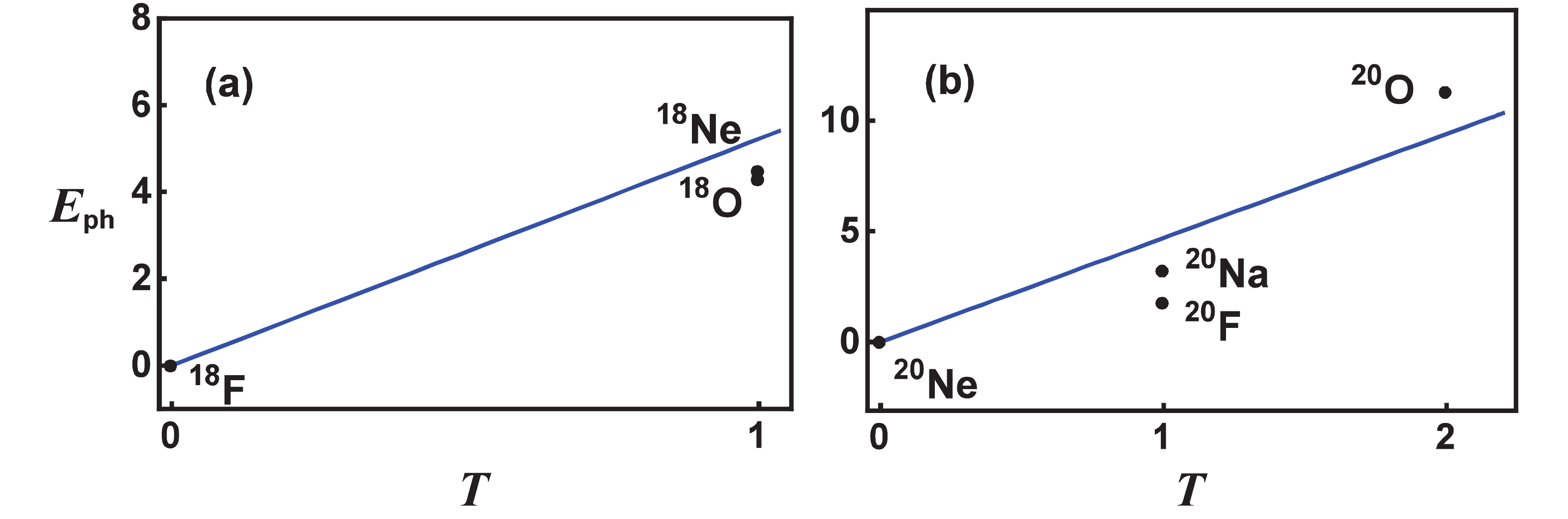

Figure 3.  (color online) The contribution of the particle-hole interaction in MeV (dots) in the binding energy relative to that of $ ^{18}{\rm{F}} $ [panel (a)] and $ ^{20}{\rm{Ne}} $ [panel (b)] versus the ground state isospin T in A = 18 and 20 nuclei. The straight line represents the smooth part of the Wigner energy term in the binding energy [58] with $ E_{\rm {W}} = {47}\vert N-Z\vert/A $ MeV = $ {94} T/A $ MeV.

In this work, the competition of isovector and isoscalar pairing in $ A=18 $ and 20 even-even $ N \approx Z$ nuclei was analyzed using the mean-field plus dynamic QQ, pairing and particle-hole interaction model, whose Hamiltonian is diagonalized in the basis U$(24) \supset(U(6)\supset SU(3) \supset SO(3))$$ \otimes (U(4)\supset SU _{S}(2) \otimes SU_{T}(2) )$ restricted to the $ L = 0 $ configuration subspace. This may be an approximation for a few lowest $ J = 0 $ and $ J = 1 $ levels, where multi-particle and multi-hole excitations are not considered. It was shown that the QQ and particle-hole interactions also play a significant role in determining the relative positions of low-lying excited $ 0^+ $ and $ 1^+ $ levels and their energy gaps, which can result in the ground state first-order quantum phase transition from $ J = 0 $ to $ J = 1 $. The strengths of the isovector and isoscalar pairing interactions in these even-even nuclei were estimated with respect to the energy gap and the total contribution to the binding energy. It was shown that the ratio of the strengths of the isoscalar and the isovector pairing interactions is about $ 1.8 $ in $ ^{18}{\rm{F}} $, and about 0.82−0.96 in A = 20 $ N \approx Z$ nuclei. Most importantly, it was shown that although the mechanism of particle-hole contribution to the binding energy is different, it is indirectly related to the Wigner term in the binding energy. This was clearly shown by the contribution of the particle-hole interaction to the binding energy relative to that of $ ^{18}{\rm{F}} $ and $ ^{20}{\rm{Ne}} $ in the A = 18 and A = 20 $ N \approx Z$ nuclei compared to the Wigner energy term. Since the analysis was restricted to the $ L = 0 $ configuration subspace, only a rough estimate of the isovector and isoscalar pairing could be made. Similar calculations using the same model in a larger subspace, for example in the entire ds and pf shells, and with multiple particle-hole excitations, could be carried out, from which more accurate information about the isovector and isoscalar pairing would be available. This approach will be considered in our future work.