


 Abstract
 HTML
HTML Reference
 Related
 PDF
PDF


-
The accumulated astrophysical evidence in favor of the cold dark matter hypothesis is currently one of the main reasons to study extensions of the Standard Model (SM). A very popular construction in this area is to consider a second scalar field transforming as a doublet of
$ SU(2)_{L} $ , supplemented by an unbroken$ Z_{2} $ symmetry. This is the so called “Inert Two Higgs Doublet Model” (i2HDM) [1-3]. Recently, motivated by the hypothesis that dark matter belongs to a complex sector with its own set of non-Abelian interactions, our group studied a modified version of i2HDM , where the standard sector and the inert scalar doublet transform under different local$ SU(2) $ groups [4]. This setup may arise, for instance, if the dark matter is a composite state. In this case, the new$ SU(2) $ corresponds to a local hidden symmetry that dynamically emerges from an underlying strong interacting sector (that is not specified in our effective model) . The gauge bosons of this effective$ SU(2) $ local group give rise to the dark vector resonances which are the next massive composite particles. This construction is a direct analogy of the description of pions and rho meson in the usual hadron physics.As we will see in the next section, the resulting model is at low energy just i2HDM with extra massive vector resonances, which couple weakly to the standard sector but strongly to the new scalars. Our previous study showed that the new resonances introduce important modifications of the observables, like the predicted relic density of the dark matter candidate [4]. Moreover, we also learned that the eventual detection of the vector resonances at the LHC is a very challenging task, even in the high luminosity regime. For this reason, it seems wise to study the possibility of detection of these resonances in future accelerators, specially in the clean environment of the planned lepton colliders. However, of the future electron-positron colliders, only CLIC is planned to run at an energy high enough (
$ \sqrt{s} = 3 $ TeV) to explore the mass range we expect for the vector resonance (overviews of CLIC and its possibility to search for new physics can be found in [5-10]). Additionally, the projected integrated luminosity (2 ab−1) promises an adequate scenario for discovering subtle effects like the existence of a dark resonance.In this work, we study the possibility of discovering the non-Abelian vector resonances at CLIC. The paper is organized in the following way. In Section 2, we briefly describe our model, emphasizing the new vector sector. Then, in Section 3, we describe our analysis and our results. Finally, in Section 4, we state our conclusions.
-
Our model is an extension of the Inert Two Higgs Doublet Model and is based on the gauge group
$ SU(2)_{1}\times SU(2)_{2}\times U(1)_{Y} $ . Our construction has been completely described in [4] and here we only recall its most important aspects.The standard sector (including a scalar doublet) is assumed to transform only under
$ SU(2)_{1} $ and$ U(1)_{Y} $ , while a second scalar doublet transforms under$ SU(2)_{2} $ (and$ U(1)_{Y} $ ). The breakdown of$ SU(2)_{1}\times SU(2)_{2} $ to the standard$ SU(2)_{L} $ is described by a non-linear link field$ \Sigma $ , which transforms as a bi-doublet under$ SU(2)_{1}\times SU(2)_{2} $ . The Lagrangian describing the bosonic sector of the model can be written as$ \begin{split} {\cal{L}} =& -\frac{1}{2}Tr\left[F_{1\mu\nu}F_{1}^{\mu\nu}\right]-\frac{1}{2}Tr\left[F_{2\mu\nu}F_{2}^{\mu\nu}\right]-\frac{1}{4}\left[B_{\mu\nu}B^{\mu\nu}\right] \\& +\frac{u^{2}}{2}Tr\left[\left(D_{\mu}\Sigma\right)^{\dagger}\left(D^{\mu}\Sigma\right)\right] + \left(D_{\mu}\phi_{1}\right)^{\dagger}\left(D^{\mu}\phi_{1}\right)\\&+\left(D_{\mu}\phi_{2}\right)^{\dagger}\left(D^{\mu}\phi_{2}\right)-m_{1}^{2}\left(\phi_{1}^{\dagger}\phi_{1}\right)-m_{2}^{2}\left(\phi_{2}^{\dagger}\phi_{2}\right) \\ &+ \lambda_{1}\left(\phi_{1}^{\dagger}\phi_{1}\right)^{2}+\lambda_{2}\left(\phi_{2}^{\dagger}\phi_{2}\right)^{2}+\lambda_{3}\left(\phi_{1}^{\dagger}\phi_{1}\right)\left(\phi_{2}^{\dagger}\phi_{2}\right) \\ & + \lambda_{4}\left(\phi_{1}^{\dagger}\Sigma\phi_{2}\right)\left(\phi_{2}^{\dagger}\Sigma^{\dagger}\phi_{1}\right)+\frac{\lambda_{5}}{2}\left[\left(\phi_{1}^{\dagger}\Sigma\phi_{2}\right)^{2}+\left(\phi_{2}^{\dagger}\Sigma^{\dagger}\phi_{1}\right)^{2}\right] \end{split}, $

(1) where
$ A_{1\mu} $ and$ A_{2\mu} $ are the gauge bosons of$ SU(2)_{1} $ and$ SU(2)_{2} $ , respectively, and$ B_{\mu\nu} = \partial_{\mu}B_{\nu}-\partial_{\nu}B_{\mu} $ is the field strength tensor of$ U(1)_{Y} $ . The scalar doublets are denoted by$ \phi_{1} $ and$ \phi_{2} $ , and their covariant derivatives are:$ D_{\mu}\phi_{j} = \partial_{\mu}\phi_{j}-ig_{j}A_{j\mu}\phi_{j}-i \displaystyle\frac{g_{Y}}{2}B_{\mu}\phi_{j}\;\;{\rm{ with }}\;\; j = 1,2 $

(2) and the derivative of the link field is:
$ D_{\mu}\Sigma = \partial_{\mu}\Sigma-ig_{1}A_{1\mu}\Sigma+ig_{2}\Sigma A_{2\mu}. $

(3) The standard fermions, on the other hand, couple to the gauge bosons of
$ SU(2)_{1} $ and$ U(1)_{Y} $ , and to$ \phi_{1} $ , as in SM.After the original symmetry breaking process, which we assume to happen at a scale
$ u $ larger than the electroweak scale$ v $ , the Lagrangian can be written in the unitary gauge ($ \Sigma = 1 $ ) as:$ \begin{split} {\cal{L}} =&-\frac{1}{2}Tr\left[F_{1\mu\nu}F_{1}^{\mu\nu}\right]-\frac{1}{2}Tr\left[F_{2\mu\nu}F_{2}^{\mu\nu}\right]-\frac{1}{4}\left[B_{\mu\nu}B^{\mu\nu}\right] \\ &+ \displaystyle\frac{u^{2}}{2}Tr\left[\left(g_{1}A_{1\mu}-g_{2}A_{2\mu}\right)\left(g_{1}A_{1}^{\mu}-g_{2}A_{2}^{\mu}\right)\right] \\ & + \left(D_{\mu}\phi_{1}\right)^{\dagger}\left(D^{\mu}\phi_{1}\right)+\left(D_{\mu}\phi_{2}\right)^{\dagger}\left(D^{\mu}\phi_{2}\right)+m_{1}^{2}\left(\phi_{1}^{\dagger}\phi_{1}\right)\\ &+m_{2}^{2}\left(\phi_{2}^{\dagger}\phi_{2}\right) - \lambda_{1}\left(\phi_{1}^{\dagger}\phi_{1}\right)^{2}-\lambda_{2}\left(\phi_{2}^{\dagger}\phi_{2}\right)^{2}-\lambda_{3}\left(\phi_{1}^{\dagger}\phi_{1}\right)\left(\phi_{2}^{\dagger}\phi_{2}\right) \\ & - \lambda_{4}\left(\phi_{1}^{\dagger}\phi\right)\left(\phi_{2}^{\dagger}\phi_{1}\right)-\frac{\lambda_{5}}{2}\left[\left(\phi_{1}^{\dagger}\phi_{2}\right)^{2}+\left(\phi_{2}^{\dagger}\phi_{1}\right)^{2}\right]. \end{split} $

(4) As usual, the electroweak symmetry is spontaneously broken when
$ \phi_{1} $ acquires a vacuum expectation value (vev)$ \left\langle \phi_{1}\right\rangle = (0,v/\sqrt{2})^{T} $ . We assume that$ \phi_{2} $ does not get a vev, and consequently, the Lagrangian remains invariant under the$ Z_{2} $ transformation$ \phi_{2}\rightarrow-\phi_{2} $ .In the limit where the coupling constant associated to
$ SU(2)_{2} $ ($ g_{2} $ ) is much larger than the one associated to$ SU(2)_{1} $ ($ g_{1} $ ), the physical vector fields can be written in terms of the gauge eigenstates as follows:$ \begin{aligned} A_{\mu} = \frac{g_{Y}}{\sqrt{g_{1}^{2}+g_{Y}^{2}}}A_{1\mu}^{3}+\frac{g_{1}g_{Y}}{g_{2}\sqrt{g_{1}^{2}+g_{Y}^{2}}}A_{2\mu}^{3}+\frac{g_{1}}{\sqrt{g_{1}^{2}+g_{Y}^{2}}}B_{\mu} \;\;\end{aligned}, $

(5) $ \begin{aligned} Z_{\mu} = -\frac{g_{1}}{\sqrt{g_{1}^{2}+g_{Y}^{2}}}A_{1\mu}^{3}-\frac{g_{1}^{2}}{g_{2}\sqrt{g_{1}^{2}+g_{Y}^{2}}}A_{2\mu}^{3}+\frac{g_{Y}}{\sqrt{g_{1}^{2}+g_{Y}^{2}}}B_{\mu} \end{aligned}, $

(6) $ \begin{aligned} \rho_{\mu}^{0} = -\frac{g_{1}}{g_{2}}A_{1\mu}^{3}+A_{2\mu}^{3}, \quad\quad\quad\quad\quad\quad\quad\quad\quad\quad\quad\quad\quad\;\; \;\;\end{aligned}$

(7) and
$ \begin{aligned} W_{\mu}^{\pm} = A_{1\mu}^{\pm}+\frac{g_{1}}{g_{2}}A_{2\mu}^{\pm} \end{aligned}, $

(8) $ \begin{aligned} \rho_{\mu}^{\pm} = -\frac{g_{1}}{g_{2}}A_{1\mu}^{\pm}+A_{2\mu}^{\pm} \end{aligned}, $

(9) where
$ \rho_{\mu}^{0,\pm} $ designates the new vector resonances, and as usual,$ A_{n\mu}^{\pm} = \displaystyle\frac{1}{\sqrt{2}}\left(A_{n\mu}^{1}\mp i A_{n\mu}^{2}\right) $ . In the same limit, the masses of the vector states can me expressed as:$ \begin{array}{l} M_A=0, \qquad {\rm{(exact)}} \end{array} $

(10) $ \begin{aligned} M_Z\approx \frac{v\sqrt{g_{1}^{2}+g_{y}^{2}}}{2}\left[1-\frac{1}{2}\frac{g_{1}^{4}}{g_{2}^{2}(g_{1}^{2}+g_{y}^{2})}\right] \end{aligned}, $

(11) $ \begin{aligned} M_{\rho^0}\approx \frac{a v g_2}{2}\left[1+\frac{g_1^2}{2g_2^2} \right] \end{aligned}, $

(12) $ \begin{aligned} M_{W}\approx\frac{v g_1}{2}\left[1-\frac{g_1^2}{2g_2^2} \right] \end{aligned}, $

(13) $ \begin{aligned} M_{\rho{\pm}}\approx \frac{a v g_2}{2}\left[1+\frac{g_1^2}{2g_2^2} \right] \end{aligned}. $

(14) Note that the interaction of the dark sector with the standard sector is suppressed by a factor
$ g_{1}/g_{2} $ . Consequently, large values of$ g_{2} $ , and vector resonances with masses above 2 TeV, make the new sector invisible in the current LHC searches [11-13].In the scalar sector, the spectrum is straightforward since no mass mixing term arises due to the
$ Z_{2} $ symmetry. Consequently, near the minimum of the potential, the scalar doublets can be parametrized as:$ \phi_{1} = \frac{1}{\sqrt{2}}\left(\begin{array}{c} 0\\ v+H \end{array}\right)\qquad\phi_{2} = \frac{1}{\sqrt{2}}\left(\begin{array}{c} \sqrt{2}h^{+}\\ h_{1}+ih_{2} \end{array}\right). $

(15) Note that the
$ Z_{2} $ symmetry makes the lightest new scalar stable (which we assume to be$ h_{1} $ ) , and a dark matter candidate [4]. For this reason, we call the new sector (formed by$ \rho_{\mu}^{0,\pm} $ ,$ h_{1} $ ,$ h_{2} $ and$ h^{\pm} $ ) the "dark sector".The model described above has several new parameters, such as the masses of the new vector and scalar states, the scale
$ u $ , and the parameters of the scalar potential. However, for this work, the only relevant free parameters of the model are the masses of the vector resonances ($ M_{\rho} $ ), the masses of the new scalars ($ m_{h1} $ ,$ m_{h2} $ and$ m_{h\pm} $ ) and$ a\equiv u/v $ . In what follows, we will take$ a = 3,4,5 $ and$ M_{\rho}\in [2,3] $ TeV, since in this way we keep$ g_{1}/g_{2}\lesssim 0.2 $ , which is consistent with our level of approximation. The chosen values of$ a $ are the same as already considered in our previous work on dark matter phenomenology [4]. They are also representative of low, moderate and high composite scale in the dark sector, given the values of$ M_{\rho} $ .The model reproduces the observed relic density provided that
$ M_{h1}<M_{\rho} $ -
The aim of this work is to study the possibility of discovering the new vector resonance
$ \rho_{\mu} $ at the future lepton collider CLIC. The basic idea is to take profit from its high energy ($ \sqrt{s} = 3 $ TeV), its expected high integrated luminosity ($ {\cal L}\approx2\;{\rm{ab}}^{-1}$ ) , and to use the effects of initial state radiation and radiative return to the resonance in order to scan the relevant range of possible$ \rho $ mass values:$ M_{\rho}\in[2,3] $ TeV. The upper limit of this interval is determined by the maximum center-of-mass energy available at CLIC, while the lower limit makes sure that the resonance has escaped detection at the LHC [4,11-13]. We focus on the process$ e{^+}e^{-}\rightarrow\mu^{+}\mu^{-} $ which, to leading order, is described only by the interchange of a photon,$ Z $ boson and$ \rho^{0} $ in the s-channel.Our model was implemented in CalcHEP [14] using the LanHEP [15,16] package. We used CalcHEP to generate events taking into account the initial state radiation with the accelerator parameters given by the Particle Data Group [17] and listed in the Table 1.
parameter value maximum beam energy 1.5 TeV bunch length 4.4×10⁻³ cm beam radius H: 4.5×10⁻² μm V: 9×10⁻⁴ μm particles per bunch 0.37×10¹⁰ luminosity 6×1034 cm−2s-1 Table 1. CLIC parameters
In this simulation, we considered the contributions of the standard sector as well as the production of a dark resonance. We smeared the momenta of the events generated with CalcHEP using a Gaussian distribution in order to take into account the finite momentum resolution of the detector. For this purpose, we use
${\Delta p}/{p} = 0.05 $ . We then computed the invariant mass of the$ \mu^{+}\mu^{-} $ pair in an interval around the (expected) mass of the resonance. Finally, we fitted the spectrum with a Gaussian resonance and a quadratic background in order to obtain the number of resonant events and the number of background events. All our simulations were performed to leading order and we considered only the irreducible background. An additional limitation of our methodology is that we considered only the local statistical analysis of the resonance, in the sense that the computed statistical significance of the signal refers only to the local significance and not to the global one.As was already pointed out in [4], the possibility of discovering the new vector bosons in a resonant process depends on whether they can decay or not into the new scalars. The reason behind this feature is that we are assuming that the coupling constant
$ g_{2} $ is large (in order to guarantee small interactions with the standard sector), making the "dark sector" strongly coupled. Consequently, two kinematic regimes open up, depending on whether the masses of the new scalars are larger or smaller than$ M_{\rho}/2 $ . We call them the Heavy Scalars and Light Scalars scenarios, respectively. In fact, the partial decay widths of$ \rho^{0} $ (which are relevant for the process we are studying) are given by:$ \begin{aligned} \Gamma\left(\rho^{0}\rightarrow\bar{f}f\right) = N_{c}\frac{a^{2}M_{W}^{4}}{24\pi v^{2}M_{\rho}^{4}}\left(M_{\rho}^{2}-m_{f}^{2}\right)\sqrt{M_{\rho}^{2}-4m_{f}^{2}} \end{aligned}, $

(16) $ \begin{aligned} \Gamma\left(\rho^{0}\!\rightarrow\! h_{1}h_{2}\right) \!= \! \frac{\left[M_{\rho}^{2}\!-\!\left(m_{h1}\!+\!m_{h2}\right)^{2}\right]^{3/2}}{48\pi a^{2}v^{2}M_{\rho}^{3}}\left[M_{\rho}^{2}\!-\!\left(m_{h1}\!-\!m_{h2}\right)^{2}\right]^{3/2} \end{aligned}, $

(17) $ \begin{aligned} \Gamma\left(\rho^{0}\rightarrow h^{+}h^{-}\right) = \frac{1}{48\pi a^{2}v^{2}}\left[M_{\rho}^{2}-4m_{h\pm}^{2}\right]^{3/2} \end{aligned}, $

(18) $ \begin{aligned} \Gamma\left(\rho^{0}\rightarrow ZH\right) \approx \frac{a^{2}M_{W}^{4}}{48\pi v^{2}M_{\rho}} \end{aligned}, $

(19) where
$ f $ represents the standard fermion,$ N_{c} $ is the number of colors, and the last equation is given for$ M_{W}\ll M_{\rho} $ .As an example, we plot in Fig. 1 the total decay width of
$ \rho^{0} $ (with$ M_{\rho} = 2500 \;{\rm{GeV}}$ ) , for three different values of$ a $ , as a function of$ m_{h1} $ , when all non-standard scalars are degenerate. We clearly see how quickly the total width grows for$ m_{h1}<M_{\rho}/2 $ , resulting in the two kinematic regimes.
Figure 1. (color online) Width of the vector resonance (
$\rho_{\mu}$ ) as a function of the mass of the non-standard scalar, in the case they are degenerate. Here, we take$M_{\rho} = 2.5$ TeV. -
In the case of Heavy Scalars,
$ \rho^{0} $ appears as a narrow resonance (with a width of just a few GeV) in the di-muon spectrum (see Fig. 2(a)). After the smearing procedure, a broader peak is obtained (Fig. 2(b)). We fit this peak in the interval$ \left[M_{\rho}-{M_{\rho}}/{10},M_{\rho}+{M_{\rho}}/{10}\right] $ using a Gaussian function (signal) plus a quadratic polynomial (background). Then we extract the number of events for the signal and for the background by integrating the Gaussian function and the quadratic polynomial, respectively, in the interval defined above. The corresponding cross-sections are shown in Fig. 3. The error bars for the signal and the background reflect the uncertainties introduced by our Monte Carlo, the smearing of the momenta and our method of extracting the signal through a fitting procedure. On the other hand, although the signal and the background cross-sections decrease with di-muon invariant mass ($ M_{\mu\mu} $ ), the energy distribution of the electrons increases with$ \sqrt{s} $ , reaching its maximum at the nominal center-of-mass energy of$ \sqrt{s_{\max}} = 3 $ TeV. The reason for this behavior is that the events with low energy electrons are due to the initial state radiation. Additionally, the interval where the resonance is fitted and integrated increases with$ M_{\rho} $ . All these effects produce the$ M_{\rho} $ dependence of the signal and background cross-sections observed in Fig. 3. Note that in Fig. 3(b) the backgrounds obtained for different sets of data (different values of$ a $ ) almost coincide. This feature shows the self-consistency of our fitting procedure.
Figure 2. (color online) Example of a resonace in the di-muon invariant mass spectrum with (right) and without (left) smearing.
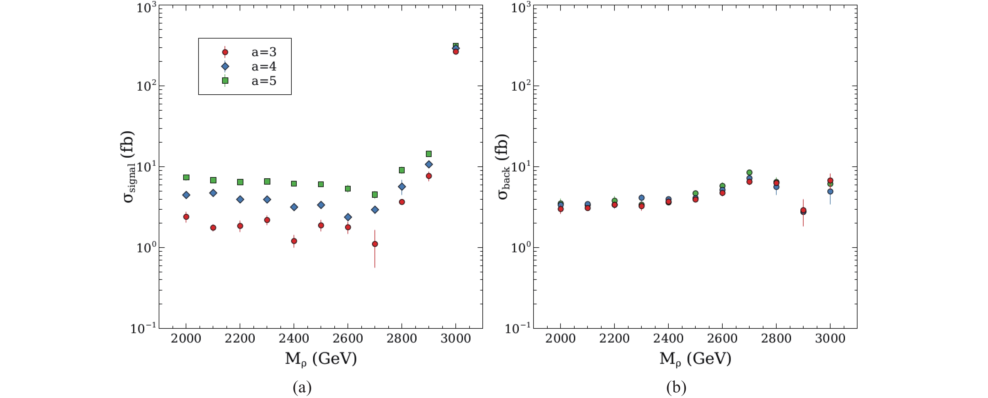
Figure 3. (color online) Signal (left) and background (right). The error bars reflect the variability introduced by our Monte Carlo and smearing procedures.
We see that the signal (Fig. 3(a)) and background (Fig. 3(b)) cross-sections are of the same order of magnitude, and the expected excess of events (for the projected integrated luminosity) should be clearly observable. Indeed, using the usual definition of the statistical significance
$ S = \frac{{\cal L}\sigma_{\rm{signal}}}{\sqrt{\cal{L}\sigma_{\rm{signal}}+\cal{L}\sigma_{\rm{background}}}}, $

(20) we estimate the integrated luminosity needed to get to the discovery criteria
$ S = 5 $ . The result is shown in Fig. 4. Note that the needed integrated luminosity is in all cases much smaller than the maximum integrated luminosity expected at CLIC of 2000 fb−1.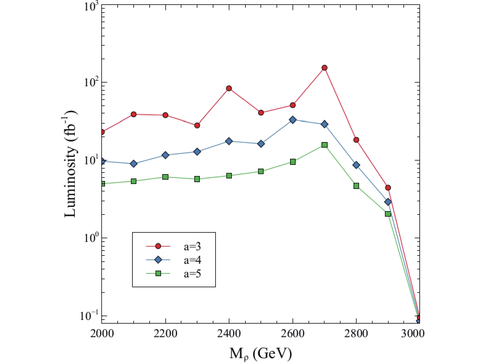
Figure 4. (color online) Integrated luminosity needed to obtain a (local) significance of 5.
-
As explained above, when the non-standard scalars are light,
$ \rho^0 $ becomes broad and in general it is difficult to identify it as a proper resonance. Indeed, after the smearing process, we could fit a resonance only in the case of$ a = 5 $ , so that in this scenario we restrict to this value of$ a $ . An example of such a resonance is shown in Fig. 5.
Figure 5. (color online) Example of a resonance obtained in the case of light scalars. Here we take
$ M_{\rho} = 2500 $ GeV,$ m_{h1} = m_{h2} = m_{h\pm} =$ 1150 GeV and$ a = 5 $ .However, this region of the parameter space is worth exploring. In doing so we found three important alternatives: 1) when one neutral scalar (the DM candidate) is the only light scalar, 2) when both neutral scalars are light and the charged ones remain heavy, and 3) when all non-standard scalars are light. In the following subsections we comment these alternatives. For the convenience of the discussion, we define a new parameter (
$ \delta m $ ) as$ \delta m \equiv M_{\rho}/2-m_{\rm LS}, $

(21) where
$ m_{\rm LS} $ is the mass of the light scalar.Similarly to the previous case, we fit the spectrum and identify the resonant and background events. The only difference is that this time we fit the resonance and the background in the interval
$ \left[M_{\rho}\!-\!{M_{\rho}}/{5},M_{\rho}\!+\!{M_{\rho}}/{5}\right] $ . -
When only one scalar is light, the neutral vector resonance (
$ \rho_{0} $ ) cannot decay into the non-standard scalars since in our model there are no$ \rho h_1 h_1 $ or$ \rho h_2 h_2 $ interaction terms, only the$ \rho h_1 h_2 $ term. Hence, this case is equivalent to the case analyzed in the previous subsection. -
When the two neutral scalars are light (but the charged ones remain heavy) the widths of the vector resonances moderately increase. For a given value of
$ M_{\rho} $ , we were able to identify resonances provided that$ \delta m\lesssim 250 $ GeV. In Fig. 6, we show the cross-sections for the signal and the background for two situations: a) as a function of$ M_{\rho} $ , while keeping$ \delta m = 100 $ GeV , and b) as a function of the mass of the (degenerate) scalars, while keeping$ M_{\rho} = 2500 $ GeV. Although the signal is systematically smaller than the background, the signal over background ratio takes acceptable values ($ 0.1 \lesssim S/B \lesssim 0.5 $ ).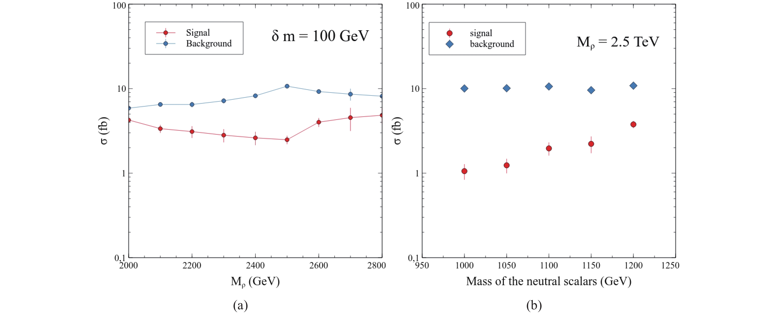
Figure 6. (color online) Signal and background cross-sections for (a)
$ \delta m = 100 $ GeV and$ M_{\rho} \in [2,3] $ TeV, and (b)$ M_{\rho} = 2.5 $ TeV, and the mass of the neutral scalars in the range$ [950, 1250] $ GeV. In both cases, we consider that the non-standard neutral scalars are degenerate while the charged ones remain heavy. In both plots, we use$ a = 5 $ . -
In the following paragraphs, we explore the case where all scalars are degenerate, which is compatible with dark matter phenomenology. Indeed, our previous study showed that the model reproduces the experimental information better when the mass difference between
$ h_1 $ and the other scalars is of the order of a few GeV. Of course, such a small mass difference is not important for our collider simulations.In Fig. 7 , we show the computed cross-sections for the signal and the background for: (a)
$ \delta m = 100 $ GeV and$ M_{\rho} \in [2,3] $ TeV, and (b)$ M_{\rho} = 2.5 $ TeV and the mass of the scalars in the range$ [1110, 1230] $ GeV. The signal is again systematically smaller than the background, but still comparable. At the maximum integrated luminosity, a few thousand signal events could be expected. As in the previous case, we compute the integrated luminosity needed for reaching the discovery level. The results are shown in Fig. 8.
Figure 7. (color online) Signal and background cross-sections for (a)
$ \delta m = 100 $ GeV and$ M_{\rho} \in [2,3] $ TeV, and (b)$ M_{\rho} = 2.5 $ TeV and the mass of the scalars in the range$ [1110, 1230] $ GeV. In both cases, we consider that all non-standard scalars are degenerate. In both plots, we use$ a = 5 $ .
Figure 8. (color online) Integrated luminosity needed to obtain a significance of 5 in the case of light scalars and
$ a = 5 $ .In summary, there is some discovery potential (although reduced) in the channel
$ e^+ e^- \rightarrow \mu^+ \mu^- $ when all scalars are light, at least when the scale of the vector resonance is high ( i.e. when$ a = 5 $ ). However, for light scalars a more promising possibility arises through the$ e^+ e^- \rightarrow h^+ h^- $ channel. In Fig. 9 , we plot the production cross-section for the pair$ h^+ h^- $ for different values of$ M_{\rho} $ assuming that the mass of the scalars is$m_{h1} = m_{h2} = $ $ m_{h\pm} = M_{\rho}/2 - 100 $ GeV. For all values of$ a $ considered we found that the cross-sections in this channel are significantly higher than in the di-muon channel. Even the new vector resonance may be observable in the invariant mass distribution of$ h^+ h^- $ , as seen in Fig. 10. As a result, the pair production of charged scalars appears as an effective means of discovering the dark sector at CLIC.
Figure 9. (color online) Production cross-section for the pair
$ h^+ h^- $ (in fb) for different values of$ M_{\rho} $ . Here, we have taken the benchmark point$ m_{h1} = m_{h2} = m_{h\pm} = M_{\rho}/2 - 100 $ GeV.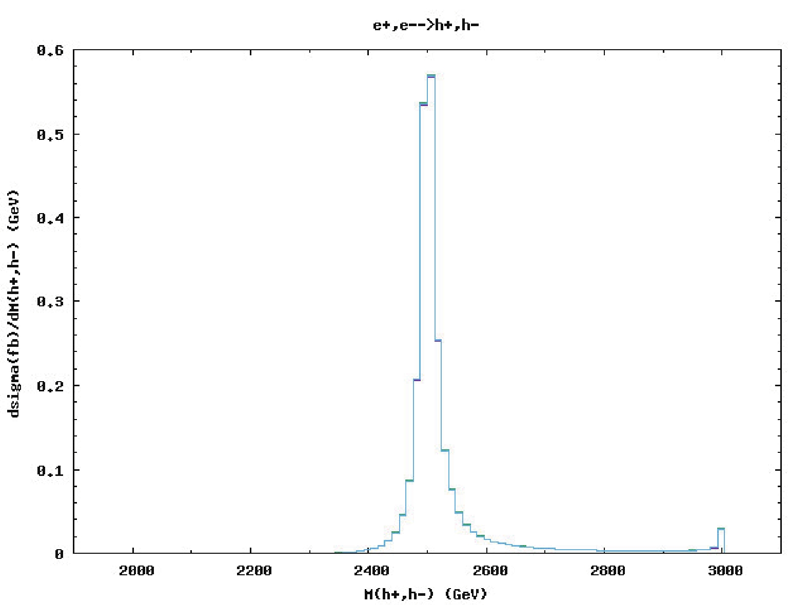
Figure 10. (color online) Invariant mass distribution of the
$ h^+ h^- $ pair for$ a = 3 $ ,$ M_{\rho} = 2500 $ GeV and$ m_{h1} = m_{h2} = m_{h\pm} = $ 1150 GeV. We observe the peak corresponding to the resonant production of$ \rho^0 $ . No smearing has been applied in this case. -
Although our main focus in this work is the study of the di-muon channel as a means for discovering the new dark resonance, in this section will briefly consider the mono-Z production. This channel is traditionally important for the search of dark matter at colliders. In our case, the main mono-Z production processes are
$ e{^+}e{^-}\rightarrow Zh_{1}h_{1} $ and$ e{^+}e{^-}\rightarrow Zh_{1}h_{2} $ , the latter being the dominant one. For this analysis, we follow the intermediate scenario where the neutral scalars are supposed to be light (in the sense explained above, that is,$ m_{h1} = m_{h2} = M_{\rho}/2-100 $ GeV ), while the charged scalars are supposed to be heavy. Interestingly, these two processes are weakly dependent on the parameter$ a $ (in fact, the resonant production$e{^+}e{^-}\rightarrow $ $ \rho\rightarrow Zh_{i}h_{j} $ is exactly independent of$ a $ ).In Fig. 11 , we show the transverse momentum distribution of the Z boson (Fig. 11(a)) , and the missing invariant mass distribution (Fig. 11(b)) for
$ e{^+}e{^-}\rightarrow Zh_{1}h_{1} $ and$ e{^+}e{^-}\rightarrow Zh_{1}h_{2} $ with$ M_{\rho} = 2.5 $ TeV without any cuts. For comparison, we include the SM distribution for$ e{^+}e{^-}\rightarrow Z\nu_{e}\bar{\nu}_{e} $ , which is the main source of background. We see that although the main component of the signal ($ Zh_{1}h_{2} $ ) has a non-trivial structure due to the resonant contribution of$ \rho_{0} $ in the s-channel, the signal is in general several orders of magnitude smaller than the background. When we apply the cuts$ P_{TZ}\geqq100 $ GeV and$ M_{\rho}-100\;{\rm{GeV}}\leqq M_{\rm{missing}}\leqq M_{\rho}+100\;{\rm{GeV}} $ (where$ P_{TZ} $ is the transverse momentum of the$ Z $ boson and$ M_{\rm{missing}} $ is the missing invariant mass) we obtain: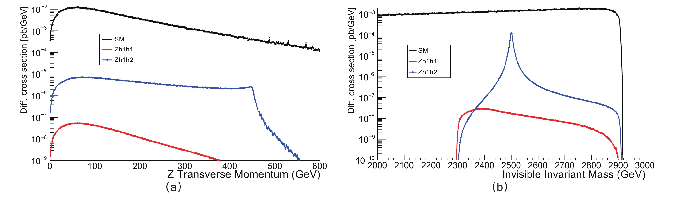
Figure 11. (color online)
$ P_{TZ} $ and the missing invariant mass distributions for$ e{^+}e{^-}\rightarrow Zh_{1}h_{1} $ and$ e{^+}e{^-}\rightarrow Zh_{1}h_{2} $ with$ M_{\rho} = 2.5 $ TeV. For comparison, we include the distribution for$ e{^+}e{^-}\rightarrow Z\nu_{e}\bar{\nu}_{e} $ predicted by the Standard Model (labeled “SM” in the pictures).$ \sigma^{\rm{signal}} = \sum_{i = 1}^{2}\sigma\left(e{^{+}}e{^{-}}\rightarrow Zh_{1}h_{i}\right)\approx\left(1.6\pm0.2\right){\rm{fb}} $

which is almost independent of the value of
$ M_{\rho} $ . On the other hand, the background cross-section with the same kinematic cuts is:$ \sigma^{\rm{back}} = \left(1.4\pm0.3\right)\times10^{2}{\rm{fb}}. $

After the cuts, the signal is still two orders of magnitude smaller than the background. However with an integrated luminosity of
$ {\cal{L}} = 2000\;{\rm{fb}}^{-1} $ the event excess will represent a statistical significance of$ S = 6 $ . This significance, however, reflects only the statistical uncertainty. A more detailed analysis should take into account the systematic uncertainties coming form the particular characteristics of the detector and the reconstruction of the Z boson, especially from its hadronic decay. An additional difficulty is due to the invisible decay of the Z boson into neutrinos. -
In this paper, we studied the possibility of using CLIC to discover a new vector resonance associated with a hypothetical strongly coupled dark sector. We focused on the di-muon production and we have strongly relied on the radiative return to the resonance. In the case where the non-standard scalars are heavy enough to forbid the decay of the vector resonances into particles of the dark sector, we predict an important excess of events for the resonance masses we considered, even when moderate smearing of the momentum is taken into account. When the scalars are light, the new vector boson becomes broad and it is difficult to define a resonance. A remarkable exception is found when the mass of the scalars is close to (but smaller than) half of the resonance mass and the scale of the dark sector is high. In all these positive cases, the high energy and high integrated luminosity projected for CLIC are sufficient for leading to the discovery of the new dark resonance, or severely constrain the model. However, for the light scalar case, the pair production of charged scalars is an attractive alternative for discovering the dark sector. In a complementary analysis, we studied the mono-Z production. We found that although this channel is more challenging than the di-muon production, after implementing an adequate cut on the missing invariant mass, the high luminosity regime of CLIC can lead to a statistically significant excess of events. These facts suggest that CLIC would be an excellent environment for testing models with a complex dark sector, and illustrate the importance of building such a machine for testing models beyond the Standard Model.
AZ is very thankful to the developers of MAXIMA [18] and the package Dirac2 [19] .These packages were used in parts of this work.
A dark vector resonance at CLIC
- Received Date: 2019-01-20
- Accepted Date: 2019-04-02
- Available Online: 2019-06-01
Abstract: One of the main problems in particle physics is to understand the origin and nature of dark matter. An exciting possibility is to consider that dark matter belongs to a new complex but hidden sector. In this paper, we assume the existence of a strongly interacting dark sector consisting of a new scalar doublet and new vector resonances, in accordance with the model recently proposed by our group. Since it was found in the previous work that it is very challenging to find the new vector resonances at the LHC, here we study the possibility of finding them at the future Compact Linear Collider (CLIC) running at


 DownLoad: