


 Abstract
 HTML
HTML Reference
 Related
 PDF
PDF


-
Since their discovery, charmonia, i.e.,
$ c\overline{c} $ mesons, have become unique tools for extending our knowledge of strong interaction dynamics at low and medium energies. In the case of lightest charmonia, their decay mechanisms can only be studied by means of effective models, since, due to their low-energy regime, these processes are beyond the perturbative description of quantum chromodynamics.We study the decays of
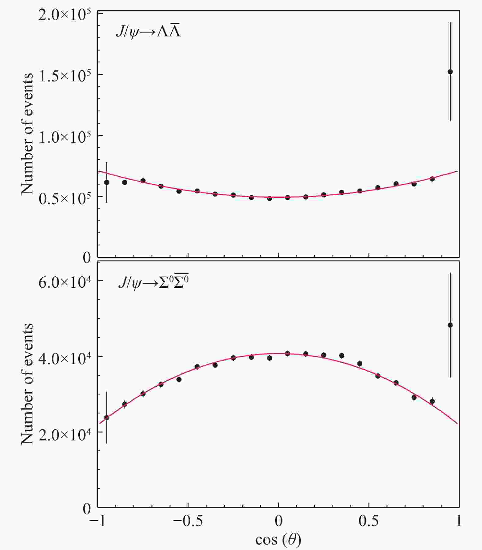
$ {{J /\psi}} $ and$ {{\psi(2S)}} $ mesons into baryon-antibaryon pairs$ {B\overline{B}} = {\Lambda\overline{\Lambda}} $ ,$ {\Sigma^0\overline{\Sigma}{}^0} $ . The differential cross section of the process$ {e^+e^-} \to \psi \to {B\overline{B}} $ has the well known parabolic expression in$ \cos\theta $ [1]$ \frac{{\rm d}N} {{\rm d} \cos \theta} \propto 1 + \alpha_B \cos^2 \theta, $

where
$ \alpha_B $ is the so-called polarization parameter and$ \theta $ is the baryon scattering angle, i.e., the angle between the outgoing baryon and the beam direction in the$ {e^+e^-} $ center-of-mass frame. As pointed out in Ref. [2], only the decay$ {{J /\psi}} \to {\Sigma^0\overline{\Sigma}{}^0} $ has a negative polarization parameter$ \alpha_B $ . Figures 1 and 2 show the BESIII data [3] for the angular distribution of the four decays:$ {{J /\psi}} \to {\Lambda\overline{\Lambda}} $ ,$ {{J /\psi}} \to {\Sigma^0\overline{\Sigma}{}^0} $ , and$ {{\psi(2S)}} \to {\Lambda\overline{\Lambda}} $ ,$ {{\psi(2S)}} \to {\Sigma^0\overline{\Sigma}{}^0} $ .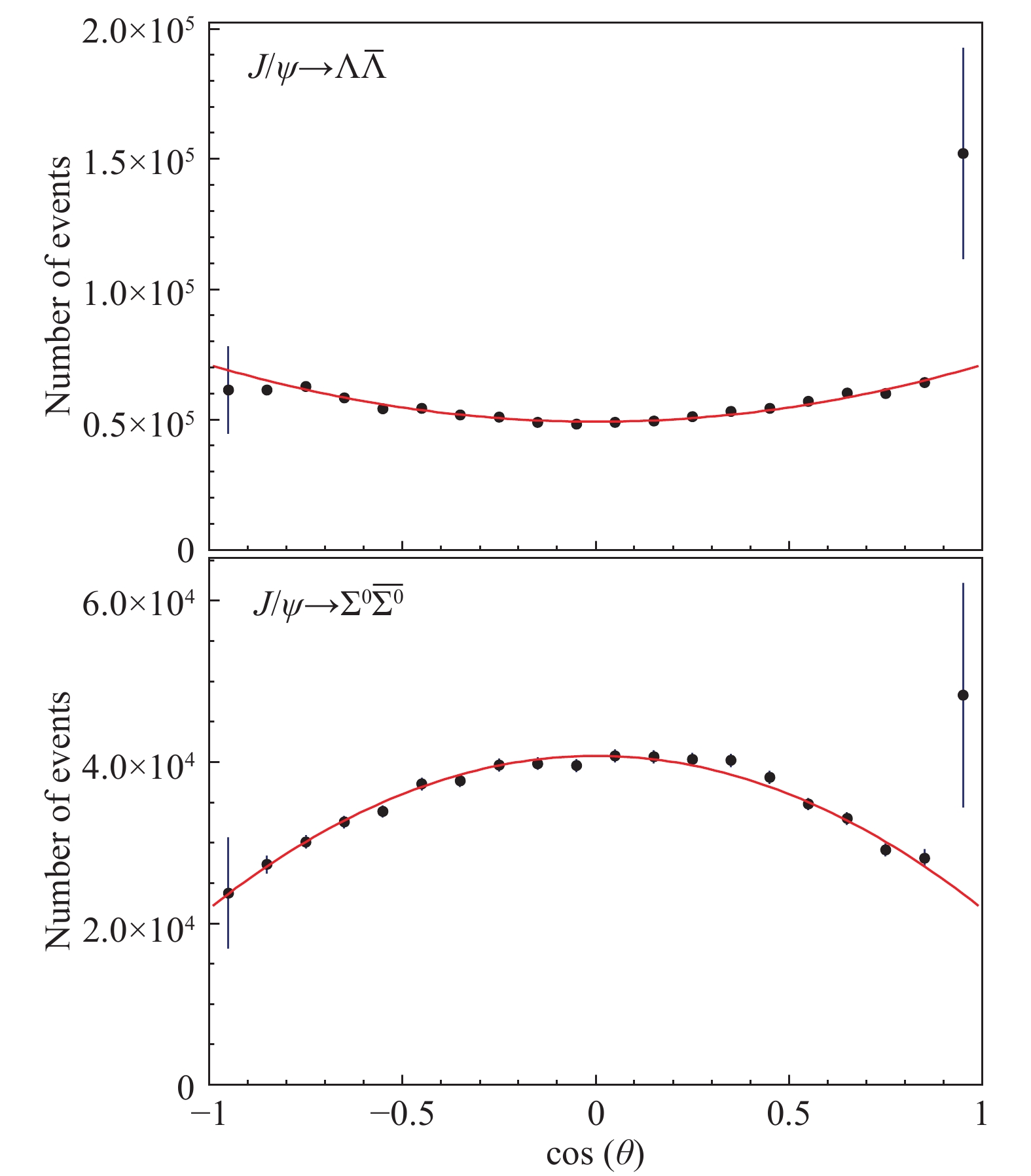
Figure 1. (color online) Angular distribution of the baryon for the
${J/\psi }$ decays into${\Lambda \bar \Lambda }$ (upper panel) and${{\Sigma ^0}{\bar \Sigma ^0}}$ (lower panel).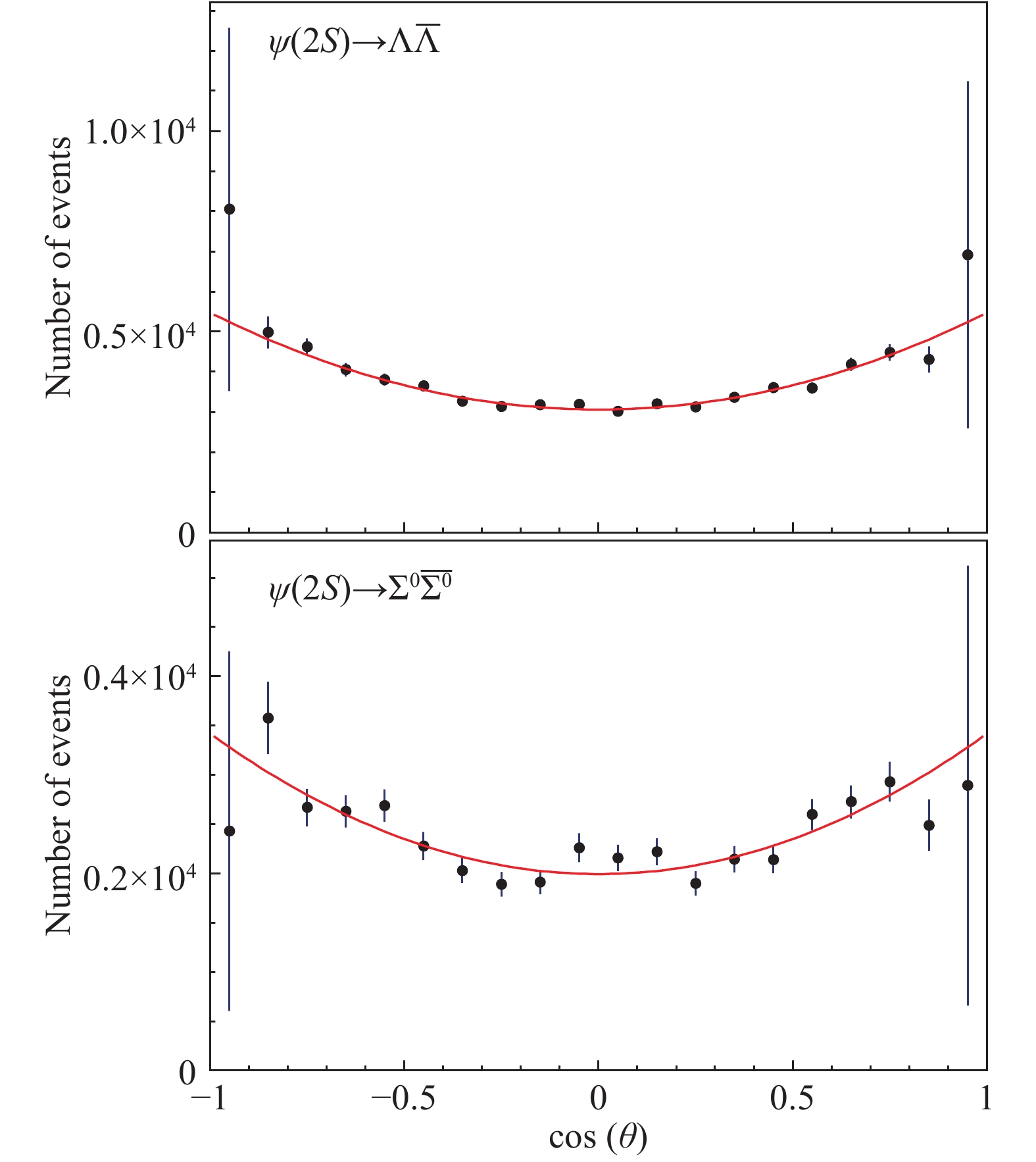
Figure 2. (color online) Angular distribution of the baryon for the
${\psi (2S)}$ decays into${\Lambda \bar \Lambda }$ (upper panel) and${{\Sigma ^0}{\bar \Sigma ^0}}$ (lower panel). -
The Feynman amplitude for the decay
$ \psi \to {B\overline{B}} $ can be written in terms of the strong magnetic and Dirac form factors as$ \mathcal{M}_{\psi\to{B\overline{B}}}=-i\epsilon_{\psi}^\mu \overline{u}(p_1)\Gamma_\mu v(p_2) $

where the matrix
$ \Gamma_\mu $ is defined in Eq. (A2),$ \epsilon_{\psi}^\mu $ is the polarization vector of the$ \psi $ meson, and the four-momenta follow the labelling of Eq. (A1). The branching ratio (BR) is given by the standard form for the two-body decay$ \mathcal{B}_{\psi\to{B\overline{B}}}={1 \over \Gamma_\psi}\frac{1}{8\pi}\overline{\left|\mathcal{M}_{\psi\to{B\overline{B}}}\right|^2}\frac{\left|\vec{p}_1\right|}{M_{\psi}^2}, $

where
$ \Gamma_\psi $ is the total width of the$ \psi $ meson. Using the mean value of the modulus squared of the amplitude, written in terms of the Sachs couplings,$\overline {{{\left| {{{\cal M}_{\psi \to B\bar B}}} \right|}^2}} = \frac{4}{3}M_\psi ^2\left( {|g_M^B{|^2} + \frac{{2M_B^2}}{{M_\psi ^2}}|g_E^B{|^2}} \right).$

we obtain the BR as
$ \mathcal{B}_{\psi\to{B\overline{B}}}=\frac{M_{\psi} \beta}{12 \pi \Gamma_\psi} \left( |g_M^B|^2 + \frac{2M_B^2}{M_{\psi}^2}|g_E^B|^2 \right) . $

(1) Since it does not depend on
$ \alpha_B $ , it cannot be used to determine the polarization parameter.The above expression for BR can be written as the sum of the moduli squared of two amplitudes
$ {\mathcal B}_{\psi\to{B\overline{B}}}=\left| A^B_M\right|^2+\left| A^B_E\right|^2, $

(2) where, comparing with Eq. (1),
$ A^B_M=\sqrt{\frac{M_{\psi} \beta}{12 \pi \Gamma_{\psi}}} g_M^B , \ \ A^B_E=\sqrt{\frac{M_{\psi} \beta}{6 \pi \Gamma_{\psi}}}\frac{M_B}{M_{\psi}} g_E^B . $

It follows that the polarization parameter of Eq. (A3) can also be written as
$ \alpha_B = {1-2|A_E^B|^2/|A_M^B|^2 \over 1+2|A_E^B|^2/|A_M^B|^2} . $

-
The SU(3) baryon octet states can be described in matrix notation as follows [4]
${O_B} = \left( {\begin{array}{*{20}{c}} {\Lambda /\sqrt 6 + {\Sigma ^0}/\sqrt 2 }&{{\Sigma ^ + }}&p\\ {{\Sigma ^ - }}&{\Lambda /\sqrt 6 - {\Sigma ^0}/\sqrt 2 }&n\\ {{\Xi ^ - }}&{{\Xi ^0}}&{ - 2\Lambda /\sqrt 6 } \end{array}} \right), $

${O_{\bar B}} = \left( {\begin{array}{*{20}{c}} {\bar \Lambda /\sqrt 6 + {{\bar \Sigma }^0}/\sqrt 2 }&{{{\bar \Sigma }^ + }}&{{{\bar \Xi }^ + }}\\ {{{\bar \Sigma }^ - }}&{\bar \Lambda /\sqrt 6 - {{\bar \Sigma }^0}/\sqrt 2 }&{{{\bar \Xi }^0}}\\ {\bar p}&{\bar n}&{ - 2\bar \Lambda /\sqrt 6 } \end{array}} \right), $

where the first matrix is for baryons and the second for antibaryons. We can consider
$ J/\psi $ and$ \psi(2S) $ mesons as SU(3) singlets. In view of the SU(3) symmetry, the zero level Lagrangian density should have the SU(3) invariant form$ \mathcal L^0 \propto {\ \rm Tr}(B \overline B) $ . Moreover, we consider two sources of SU(3) symmetry breaking: the quark mass and the EM interaction. The first can be parametrized by introducing the spurion matrix [5]$ S_m={g_m \over 3}\begin{pmatrix} 1 & 0 & 0\\ 0 & 1 & 0\\ 0 & 0 & -2\\ \end{pmatrix}, $

where
$ g_m $ is the effective coupling constant. This matrix describes the mass breaking effect due to the mass difference between$ s $ and$ u $ and$ d $ quarks, where the SU(2) isospin symmetry is assumed, so that$ m_u=m_d $ . This SU(3) breaking is proportional to the$ 8^{\rm th} $ Gell-Mann matrix$ \lambda_8 $ . The EM breaking effect is related to the fact that the photon coupling to quarks, described by the four-current$ {1 \over 2} \overline q \gamma^\mu \left( \lambda_3+\lambda_8/\sqrt{3} \right) q, $

is proportional to the electric charge. This effect can be parametrized using the following spurion matrix
$ S_e={g_e \over 3}\begin{pmatrix} 2 & 0 & 0\\ 0 & -1 & 0\\ 0 & 0 & -1\\ \end{pmatrix}, $

where
$ g_e $ is the effective EM coupling constant.The most general SU(3) invariant effective Lagrangian density is given by [5]
$\begin{split} {\cal L} = &g{\rm{Tr}}(O{O_{\bar B}}) + d{\rm{Tr}}(\{ O, {O_{\bar B}}\} {S_e}) + f{\rm{Tr}}([O{O_{\bar B}}]{S_e})\\ &+ d'{\rm{Tr}}(\{ O, {O_{\bar B}}\} {S_m}) + f'{\rm{Tr}}([O, {O_{\bar B}}]{S_m}), \end{split}$

where
$ g $ ,$ d $ ,$ f $ ,$ d' $ and$ f' $ are coupling constants. We can extract the Lagrangians describing the$ J/\psi $ and$ \psi(2S) $ decays into$ \Lambda \overline \Lambda $ and$ \Sigma^0 \overline \Sigma^0 $ ${{\cal L}_{{\Sigma ^0}{{\bar \Sigma }^0}}} = ({G_0} + {G_1}){\Sigma ^0}{\bar \Sigma ^0}, {{\cal L}_{\Lambda \bar \Lambda }} = ({G_0} - {G_1})\Lambda \bar \Lambda, $

(3) where
$ G_0 $ and$ G_1 $ are combinations of coupling constants, i.e.,$ G_0 = g, \quad G_1 = {d \over 3} (2 g_m + g_e) . $

Using the structure of Eq. (2), the BRs can be expressed in terms of the electric and magnetic amplitudes as
$\begin{aligned} {{\cal B}_{\psi \to {\Sigma ^0}{{\bar \Sigma }^0}}} &= |A_E^\Sigma {|^2} + |A_M^\Sigma {|^2}, \\ {{\cal B}_{\psi \to \Lambda \bar \Lambda }} &= |A_E^\Lambda {|^2} + |A_M^\Lambda {|^2}. \end{aligned}$

Moreover, as obtained in Eq. (3), the amplitudes can be further decomposed as combinations of leading,
$ E_0 $ and$ M_0 $ , and sub-leading terms,$ E_1 $ and$ M_1 $ , with opposite relative signs, i.e.,$\begin{aligned} {{\cal B}_{\psi \to {\Sigma ^0}{{\bar \Sigma }^0}}} &= |{E_0} + {E_1}{|^2} + |{M_0} + {M_1}{|^2}\\ & = |{E_0}{|^2} + |{E_1}{|^2} + 2|{E_0}||{E_1}|\cos ({\rho _E})\\ &\quad + |{M_0}{|^2} + |{M_1}{|^2} + 2|{M_0}||{M_1}|\cos ({\rho _M}), \\ {{\cal B}_{\psi \to \Lambda \bar \Lambda }} &= |{E_0} - {E_1}{|^2} + |{M_0} - {M_1}{|^2}\\ & = |{E_0}{|^2} + |{E_1}{|^2} - 2|{E_0}||{E_1}|\cos ({\rho _E})\\ &\quad + |{M_0}{|^2} + |{M_1}{|^2} - 2|{M_0}||{M_1}|\cos ({\rho _M}), \end{aligned}$

where
$ \rho_E $ and$ \rho_M $ are the phases of the ratios$ E_0/E_1 $ and$ M_0/M_1 $ . -
In this work, we have used the data from precise measurements [3, 6] of the branching ratios and polarization parameters, reported in Table 1, based on the events collected with the BESIII detector at the BEPCII collider. These data are in agreement with the results of other experiments [7-11]. Since for each charmonium state we have six free parameters (four moduli and two relative phases) and only four constrains (two BRs and two polarization parameters), we fix the relative phases
$ \rho_E $ and$ \rho_M $ . The values$ \rho_E=0 $ and$ \rho_M=\pi $ appear as phenomenologically favored by the data. Indeed, (largely) different phases would give negative, and hence unphysical, values for the moduli$ |E_0| $ ,$ |E_1| $ ,$ |M_0| $ and$ |M_1| $ . Moreover, as shown in Fig. 5, where the four moduli for$ J/\psi $ and$ \psi(2S) $ are represented as functions of the phases with$ \rho_E\in[-\pi/2, \pi/2] $ and$ \rho_M\in[\pi/2, 3\pi/2] $ , the obtained results are quite stable, and the central values$ \rho_E=0 $ ,$ \rho_M=\pi $ maximise the hierarchy between the moduli of leading,$ E_0 $ and$ M_0 $ , and sub-leading amplitudes,$ E_1 $ and$ M_1 $ . These values for$ |E_0| $ ,$ |E_1| $ ,$ |M_0| $ and$ |M_1| $ are reported in Table 2 and shown in Fig. 3. The corresponding values of$ |g_{E}| $ ,$ |g_{M}| $ are reported in Table 3 and shown in Fig. 4. The large sub-leading$ {{J /\psi}} $ amplitudes$ |E_1| $ ,$ |M_1| $ (see Table 2 and Fig. 3) are responsible for the inversion of the$ |g_E^B| $ ,$ |g_M^B| $ hierarchy (see Fig. 4 and Table 3).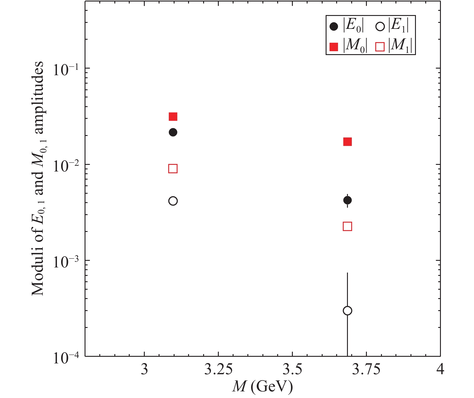
Figure 3. (color online) Moduli of the parameters from Table 2 as function of the charmonium state mass M.
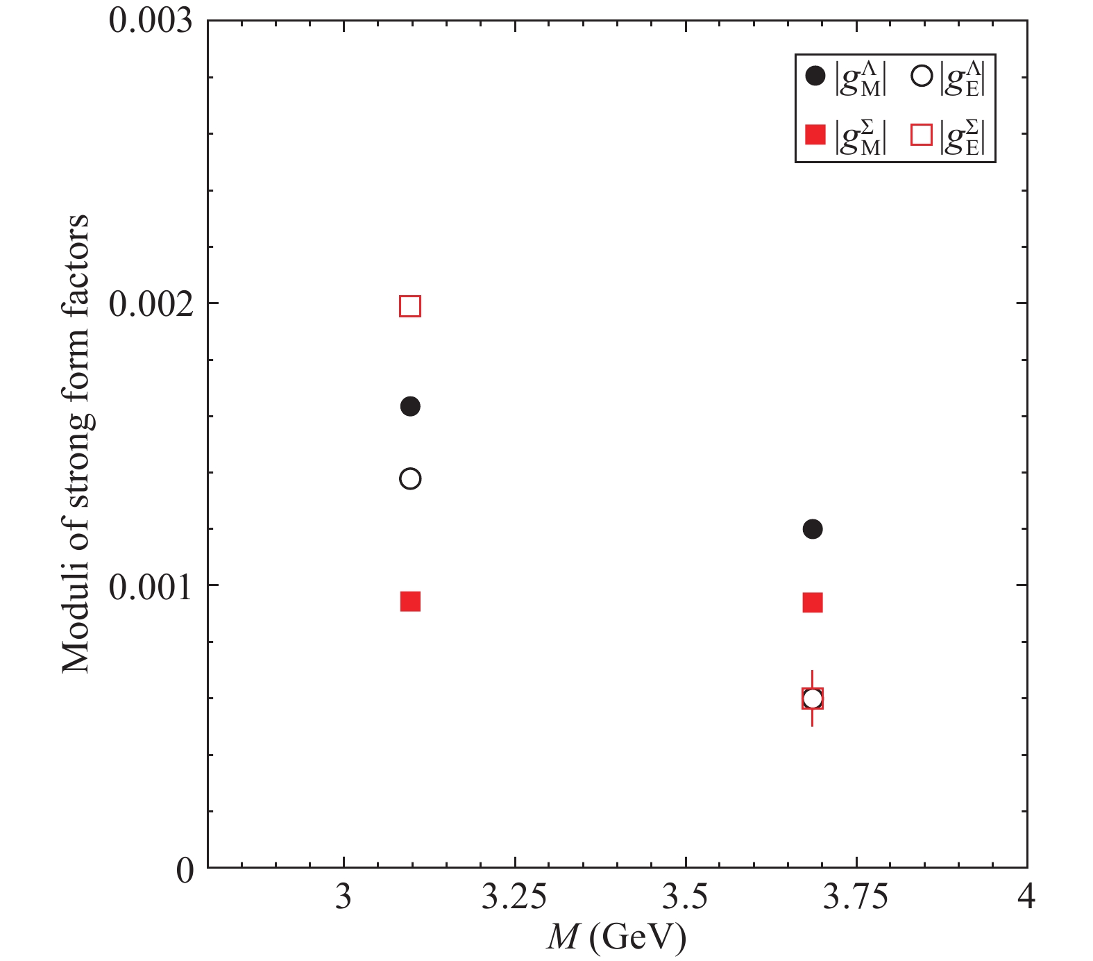
Figure 4. (color online) Moduli of the parameters from Table 3 as function of the charmonium state mass M.
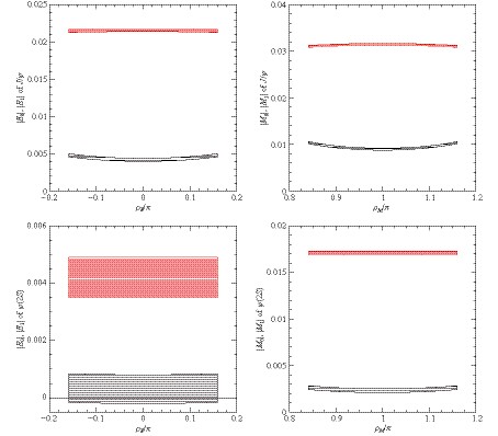
Figure 5. (color online) Red and black bands represent moduli of leading and sub-leading amplitudes, respectively. The vertical width indicates the error. Top left: moduli of amplitudes E0 and E1 for
${J/\psi}$ . Top right: moduli of amplitudes M0 and M1 for${J/\psi}$ . Bottom left: moduli of amplitudes E0 and E1 for${\psi(2S)}$ . Bottom right: moduli of amplitudes M0 and M1 for${\psi(2S)}$ .Decay BR Pol. par. ${ \alpha_B }$ 

${ J/\psi \to \Sigma^0 \overline \Sigma^0 }$ 

${ (11.64 \pm 0.04) \times 10^{-4} }$ 

${ -0.449 \pm 0.020 }$ 

${ J/\psi \to \Lambda \overline \Lambda }$ 

${ (19.43 \pm 0.03) \times 10^{-4} }$ 

${ 0.461 \pm 0.009 }$ 

${ \psi(2S) \to \Sigma^0 \overline \Sigma^0 }$ 

${ (2.44 \pm 0.03) \times 10^{-4} }$ 

${ 0.71 \pm 0.11 }$ 

${ \psi(2S) \to \Lambda \overline \Lambda }$ 

${ (3.97 \pm 0.03) \times 10^{-4} }$ 

${ 0.824 \pm 0.074 }$ 

Ampl. ${J/\psi}$ 

${\psi(2S)}$ 

${|E_0|}$ 

${(2.16 \pm 0.02) \times 10^{-2}}$ 

${(0.42 \pm 0.07) \times 10^{-2}}$ 

${|E_1|}$ 

${(0.42 \pm 0.02) \times 10^{-2}}$ 

${(0.03 \pm 0.05) \times 10^{-2}}$ 

${|M_0|}$ 

${(3.15 \pm 0.02) \times 10^{-2}}$ 

${(1.72 \pm 0.02) \times 10^{-2}}$ 

${|M_1|}$ 

${(0.90 \pm 0.02) \times 10^{-2}}$ 

${(0.23 \pm 0.02) \times 10^{-2}}$ 

Table 2. Moduli of the leading and sub-leading amplitudes.
FFs ${J/\psi}$ 

${\psi(2S)}$ 

${|g_E^\Sigma|}$ 

${(1.99 \pm 0.04) \times 10^{-3}}$ 

${(0.6 \pm 0.1) \times 10^{-3}}$ 

${|g_M^\Sigma|}$ 

${(0.94 \pm 0.02) \times 10^{-3}}$ 

${(0.94 \pm 0.02) \times 10^{-3}}$ 

${|g_E^\Lambda|}$ 

${(1.37 \pm 0.04) \times 10^{-3}}$ 

${(0.6 \pm 0.1) \times 10^{-3}}$ 

${|g_M^\Lambda|}$ 

${(1.64 \pm 0.03) \times 10^{-3}}$ 

${(1.20 \pm 0.02) \times 10^{-3}}$ 

Table 3. Moduli of the strong Sachs form factors
-
The
$ \Lambda $ and$ \Sigma^0 $ angular distributions can be explained using an effective model with the SU(3)-driven Lagrangian$ \mathcal{L}_{{\Sigma^0\overline{\Sigma}{}^0}+{\Lambda\overline{\Lambda}}} = (G_0+G_1) \Sigma^0 \overline \Sigma^0 + (G_0-G_1) \Lambda \overline \Lambda . $

The interplay between the leading
$ G_0 $ and sub-leading$ G_1 $ contributions to the decay amplitude determines the sign and value of the polarization parameter$ \alpha_B $ .In particular, the different behavior of the
$ {{J /\psi}} \to {\Sigma^0\overline{\Sigma}{}^0} $ angular distribution is due to the large values of the sub-leading amplitudes$ |E_1| $ and$ |M_1| $ . This implies that the SU(3) mass breaking and EM effects, which are responsible for these amplitudes, play a different role in the dynamics of the$ {{J /\psi}} $ and$ {{\psi(2S)}} $ decays.It is interesting to note that the angular distributions of
$ \Sigma^0(1385) $ and$ \Sigma^\pm(1385) $ , measured by BESIII [12, 13], show the same$ \Sigma^0 $ behavior.The process
$ {e^+e^-}\to{{J /\psi}}\to\Sigma^+ \overline \Sigma^- $ is currently under investigation [14]. The behavior of its angular distribution could add important information to the knowledge of the${{J /\psi}}$ decay mechanism. -
We consider the decay of a charmonium state, a
$ c \overline c $ vector meson$ \psi $ , produced via$ {e^+e^-} $ annihilation, into a baryon-antibaryon$ {B\overline{B}}$ pair, i.e., the process\scriptsize$ \tag{A1} e^-(k_1)+ e^+(k_2)\to \psi(q)\to B(p_1)+\overline{B}(p_2), $

where the 4-momenta are given in parentheses. The Feynman diagram is shown in Fig. A1 and the corresponding amplitude is
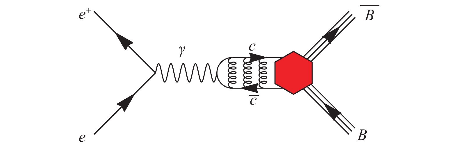
Figure A1. (color online) Feynman diagram of the process
${{e^ + }{e^ - }\! \to \psi\! \to B\bar B}$ , the red hexagon represents the${{\psi }B\bar B}$ coupling.$ { \mathcal{M}_{{e^+e^-}\to\psi\to{B\overline{B}}}=-ie^2 J_B^\mu \ D_{\psi} \left( q^2\right) \overline{v}(k_2)\gamma_\mu u(k_1), } $

where
$ J_B^\mu=\overline{u}(p_1)\Gamma^\mu v(p_2) $ is the baryonic four-current,$ D_{\psi}\left( q^2\right) $ is the$ \psi $ propagator, which includes the$ \gamma $ -$ \psi $ electromagnetic (EM) coupling, and$ \overline{v}(k_2)\gamma_\mu u(k_1) $ is the leptonic four-current. The four-momenta follow the labelling of Eq. (A1). The$ \Gamma^\mu $ matrix can be written as [15]$ \,\;\;\,\quad\quad\quad\quad\quad\quad\Gamma^\mu =\gamma^\mu f_{1}^B +\frac{i\sigma^{\mu\nu}q_\nu}{2M_B} f_2^B, \quad\quad\quad\quad\quad\quad\;\;\,\,({\rm A}2) $

where
$ M_B $ is the baryon mass and$ f_1^B $ and$ f_2^B $ are constant form factors that we call “strong” Dirac and Pauli couplings; they weigh the vector and tensor parts of the$ \psi {B\overline{B}} $ vertex①). We introduce the strong electric and magnetic Sachs couplings [16]$ g_E^B=f_1^B+\frac{M_{\psi}^2}{4M_B^2}f_2^B, \quad g_M^B=f_1^B+f_2^B, $

that have the structure of the EM Sachs form factors [17].
$ M_\psi $ is the mass of the charmonium state. The four quantities$ f_1^B $ ,$ f_2^B $ ,$ g_E^B $ and$ g_M^B $ are in general complex numbers. The differential cross section of the process$ {e^+e^-} \to \psi \to B \overline B $ in the$ {e^+e^-} $ center-of-mass frame, in terms of the two Sachs couplings, reads$ \frac{{\rm d}\sigma}{{\rm d}\cos\theta}= \frac{\pi\alpha^2 \beta}{2M_\psi^2} \left( \left|g_M^B\right|^2 + \frac{4M_B^2}{M_\psi^2}\left|g_E^B\right|^2 \right) \Big(1 + \alpha_B \cos^2 \theta \Big), $

where
$ \beta=\sqrt{1 - {4 M_B^2 \over M_{\psi}^2}} $

is the velocity of the out-going baryon at the
$ \psi $ mass,$ \theta $ is the scattering angle, and the polarization parameter$ \alpha_B $ is given by$ \quad\quad\quad\quad\quad\;\;\;\,\alpha_B =\frac{M_\psi^2\left|g_M^B\right|^2-4M_B^2|g_E^B|^2}{M_\psi^2\left|g_M^B\right|^2+4M_B^2\left|g_E^B\right|^2}, \quad\quad\quad\quad\;\;\;\,\quad({\rm A}3) $

$ \alpha_B\in[-1, 1] $ and depends only on the modulus of the ratio$ {g_E^B}/{g_M^B} $ , e.g., Fig. A2 shows the behavior of$ \alpha_\Lambda $ in the case of$ \psi={{J /\psi}} $ as function of$ |g_E^{\Lambda}|/|g_M^{\Lambda}| $ . The strong Sachs and Dirac and Pauli couplings are related through$ \alpha_B $ . Let us consider three special cases. With maximum positive polarization,$ \alpha_B=1 $ , the strong electric Sachs coupling vanishes, i.e.,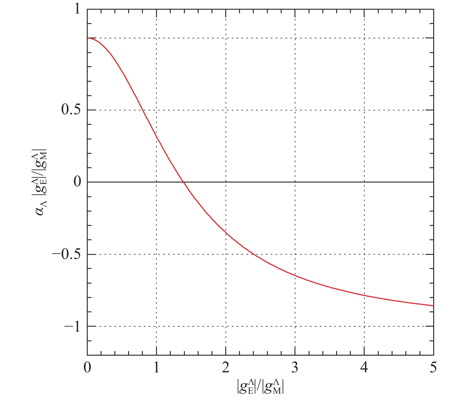
Figure A2. (color online) Polarization parameter
${\alpha_\Lambda}$ for${\psi=J/\psi}$ as function of the ratio${\left| {g_E^\Lambda } \right|/\left| {g_M^\Lambda } \right|}$ . The masses are from Ref. [18].$ \begin{split} \alpha_B&=1 \ \ \to \ \ g_E^B=0, \ \ f_1^{B} = -\frac{M_\psi^2}{4M_B^2}f_2^{B}, \\ g_M^B&=f_1^B \left( 1 -\frac{4M_B^2}{M_\psi^2} \right) = f_2^B \left( 1 -\frac{M_\psi^2}{4M_B^2} \right), \end{split} $

the relative phase between
$ f_1^B $ and$ f_2^B $ is$ i\pi $ , and the ratio of the moduli is$ M_\psi^2/(4M_B^2) $ .With maximum negative polarization we have
$ \begin{split} \alpha_B&=-1 \ \ \to \ \ g_M^B=0, \ \ f_1^{B}=-f_2^{B}, \end{split} $

$ \begin{split} g_E^B&=f_1^B \left( 1 -\frac{M_\psi^2}{4M_B^2} \right) = f_2^B \left(\frac{M_\psi^2}{4M_B^2} -1 \right), \end{split} $

so that in this case the strong magnetic Sachs coupling vanishes, the relative phase between
$ f_1^B $ and$ f_2^B $ is$ -i\pi $ and the ratio of the moduli is one.Finally, in the case with no polarization,
$ \alpha_B=0 $ , we obtain the modulus of the ratio between the Sachs couplings$ \alpha_B=0 \ \ \to \ \ \frac{|g_E^{B}|}{|g_M^{B}|}=\frac{M_\psi}{2M_B} . $

A model to explain the angular distribution of $ {{{J /\psi}}} $ and $ {{\psi(2S)}} $ decay into $ {\Lambda \overline{\Lambda}} $ and ${\Sigma^0 \overline{\Sigma^0}} $
- Received Date: 2018-10-23
- Available Online: 2019-02-01
Abstract: BESIII data show a particular angular distribution for the decay of


 DownLoad: