


 Abstract
 HTML
HTML Reference
 Related
 PDF
PDF


-
In the past decade, various exotic hadronic resonance-like structures have been observed by numerous experimental groups. These structures, due to their unknown nature, are generally called XYZ particles. The most interesting ones are the charged structures that have been discovered in both the charm and bottom sectors. These structures necessarily bear a four valence quark structure
$ \bar{Q}q\bar{q}'Q $ , where Q is a heavy flavor-quark, while q and$ q' $ are the light-flavored quarks. For different light flavors, these are charged objects. Another interesting feature is that they tend to appear close to the threshold of two heavy mesons with valence structure$ \bar{Q}q $ and$ \bar{q}'Q $ . The physical nature of these structures has been discussed in many phenomenological studies. For example, they could be shallow bound states of the two mesons due to the residual color interactions, or some genuine tetraquark objects. However, even after many phenomenological studies, the nature of many of these states remains obscure. A typical example is the structure$ Z_c(3900) $ , which is the main topic of this paper. It was first discovered by BESIII [1] and Belle [2], and soon verified by the CLEO collaboration [3]. The nature of$ Z_c(3900) $ remains open to debate. For a recent review see e.g. Refs. [4, 5]. It is therefore highly desirable that non-perturbative methods like lattice QCD could provide some information on the nature of these states.Contrary to many phenomenological studies, lattice studies of these states are still relatively rare. For the state
$ Z_c(3900) $ , it is readily observed that the invariant mass of the structure is close to the$ D\bar{D}^* $ threshold, naturally suggesting a shallow molecular bound state formed by the two corresponding charmed mesons. To further investigate this possibility, the interaction between$ D^* $ and D mesons near the threshold becomes crucial.A lattice study was performed by S. Prelovsek et al. who investigated the energy levels of the two charmed meson system in the channel where
$ Z_c $ appears in a finite volume [6]. They used quite a number of operators, including two-meson operators in the channels$ J/\psi\pi $ ,$ D\bar{D}^* $ etc. , and even tetraquark operators. However, they discovered no indication of extra new energy levels apart from the almost free scattering states of the two mesons. Taking$ D\bar{D}^* $ as the main channel, CLQCD used the single-channel Lüscher scattering formalism [7-11], and also found a slightly repulsive interaction between the two charmed mesons [12, 13]. Therefore, it is also unlikely they should form bound states. A similar study using staggered quarks also found no clue for the existence of bound states [14]. Thus, the above mentioned lattice studies, whether inspecting the energy levels alone or using the single-channel Lüscher approach, have found no clue for the existence of a$ D\bar{D}^* $ bound state.On the other hand, starting around 2015, HALQCD studied the problem using the so-called HALQCD approach [15], which is rather different from the Lüscher formalism adopted by the other groups. They claimed that this structure can be reproduced and it is not a usual bound state or resonance, but rather, a structure formed due to strong cross-channel interactions, see Refs. [16, 17] and references therein. So far, this possibility was only seen in the HALQCD approach, but not in the Lüscher-type approaches. In fact, the multi-channel Lüscher formula is known since some time [18-22], and the Hadron Spectrum Collaboration has successfully studied various coupled-channel scattering processes involving light mesons using the multi-channel Lüscher formalism [23-26]. It is therefore tempting to verify, or dispute, the cross-channel interaction scenario suggested by HALQCD in a coupled-channel Lüscher approach. More importantly, the state
$ Z_c $ has many coupled decay channels, and if the coupled-channel effects are important then inspecting the energy levels alone, or performing only a single-channel scattering study, is not sufficient to understand the nature of these structures. Therefore, in this exploratory study, we aim to make a step towards the multi-channel lattice computation using the coupled-channel Lüscher approach.It is well known that in the single-channel Lüscher approach, the energy levels are in one-to-one correspondence with the scattering phase. However, in a two-channel situation, the S-matrix is characterized by 3 parameters, all of which are functions of the scattering energy. Therefore, one needs to re-parametrize the S-matrix elements in terms of a number of constant parameters so as to pass from the energy levels to the scattering phases. One possible choice is to use the K-matrix parametrization adopted by the Hadron Spectrum Collaboration in their studies of light meson coupled-channel scattering. In this work, however, since we are only interested in the energy region very close to the threshold, we use the multi-channel effective range expansion, developed a long time ago by Ross and Shaw [27, 28]. The difficulty with the multi-channel approach lies in the fact that the number of parameters needed to parametrize the S-matrix grows quadratically with the number of channels. Therefore, based on the experimental facts and hints from the HALQCD study, we attempt to study this problem in the two-channel Lüscher approach. This could be viewed as the first step beyond the single-channel approximation using the Lüscher formalism. To be more specific, we single out the two most relevant channels for
$ Z_c(3900) $ ,$ J/\psi\pi $ and$ D\bar{D}^* $ , the first being the discovery channel for$ Z_c(3900) $ , and the second was shown to be the dominant channel in the BESIII experimental data [29]. Quite similar to the single-channel effective range expansion, which is characterized by two real parameters, namely the scattering length$ a_0 $ and the effective range$ r_0 $ , in the two-channel situation, one needs 5 real parameters to describe the Ross-Shaw matrix M: 3 for the scattering length matrix, and 2 for the effective range parameters. If one would like to go beyond two channels, these numbers go up rather quickly. For example, for the case of three channels, the scattering length matrix has 6 real parameters, while the effective range adds another 3, making a total of 9 parameters, which we think is already too many to handle. Thus, in this paper, using lattice QCD in the two-channel Lüscher formalism combined with the Ross-Shaw effective range expansion, our aim is to check whether the cross-channel interaction scenario, as suggested by the HALQCD, can be realized or not.The paper is organized as follows. In Section 2, we briefly outline the computational strategies in the Lüscher formalism, and review the Ross-Shaw effective range expansion that we use to parametrize the S-matrix elements. In particular, we discuss the conditions that should be satisfied in order to have a narrow resonance close to the threshold. In Section 3, interpolation operators are introduced from which correlation matrices can be computed. We also outline how the two most relevant channels are determined from the correlation matrix. In Section 4, calculation details are given and the results for the single- and two-meson systems are analyzed. By applying the two-channel Lüscher formula, parameters that determine the Ross-Shaw M-matrix are extracted, and the physics implied is discussed. In Section 5, we conclude with some general remarks.
-
In this section, we outline the strategies for computation described in this paper. We start by reviewing the ingredients of the Lüscher formalism with the focus on the multi-channel version. We then describe the multi-channel effective range expansion developed by Ross and Shaw. The relation of the scattering cross-section with the parameters of the Ross and Shaw theory are also outlined, which helps understand the meaning of these parameters.
-
In the original single-channel Lüscher formalism, the exact energy eigenvalue of a two-particle system in a finite box of size L is related to the elastic scattering phase of the two particles in infinite volume. For simplicity, we only consider the center-of-mass frame with periodic boundary conditions applied in all three spatial directions. Consider two interacting bosonic particles, which are called mesons in the following, with mass
$ m_1 $ and$ m_2 $ enclosed in a cubic box of size L. The spatial momentum$ { k} $ of any particle is quantized according to:$ \begin{array}{l} { k} = \left(\displaystyle\frac{2\pi}{ L}\right) { n}\;, \end{array} $

(1) with
$ { n} $ being a three-dimensional integer. The exact energy of the two-particle system in this finite volume is denoted as$ E_{1\cdot2}( { k}) $ . This can be obtained in lattice simulations from appropriate correlation functions. Defining a variable$ \bar{ { k}}^2 $ via:$ \begin{array}{l} E_{1\cdot 2}( { k}) = \sqrt{m^2_1+\bar{ { k}}^2} +\sqrt{m^2_2+\bar{ { k}}^2}\;, \end{array} $

(2) which is the energy of two freely moving particles in infinite volume with mass
$ m_1 $ and$ m_2 $ having three-momenta$ { k} $ and$ - { k} $ , respectively. It is also convenient to further define a variable$ q^2 $ as:$ \begin{array}{l} q^2 = \bar{ { k}}^2L^2/(2\pi)^2\;, \end{array} $

(3) which differs from
$ { n}^2 $ due to the interaction between the two particles. The single-channel Lüscher formula gives a direct relation between$ q^2 $ and the elastic scattering phase shift$ \tan\delta(q) $ in infinite volume: [10]$ \begin{array}{l} q\cot\delta_0(q) = \displaystyle\frac{1}{ \pi^{3/2}} {\cal Z}_{00}(1;q^2)\;, \end{array} $

(4) where
$ {\cal Z}_{00}(1;q^2) $ is the zeta-function, which can be evaluated numerically once its argument$ q^2 $ is given. This relation can also address the issue of bound states, which is related to the phase shift$ \delta(k) $ analytically continued below the threshold, see e.g. Ref. [10].For the two-channel case, the S-matrix now becomes a
$ 2\times 2 $ matrix in channel space. For example, for the strong interaction, the S-matrix is usually expressed as,$ \begin{array}{l} S = \left[\begin{array}{cc} \!\!S_{11} & S_{12}\!\!\\ \!\!S_{12} & S_{22}\!\! \end{array}\right] = \left[\begin{array}{cc} \eta {\rm e}^{2{\rm i}\delta_1} & i\sqrt{1-\eta^2}{\rm e}^{{\rm i}(\delta_1+\delta_2)}\\ i\sqrt{1-\eta^2}{\rm e}^{{\rm i}(\delta_1+\delta_2)} & \eta {\rm e}^{2{\rm i}\delta_2} \end{array}\right]\;, \end{array} $

(5) where
$ \delta_1 $ and$ \delta_2 $ are scattering phases in channel 1 and 2, respectively, and$ \eta\in[0,1] $ is the inelasticity parameter. Note that all three parameters,$ \delta_1 $ ,$ \delta_2 $ and$ \eta $ , are functions of energy. It is known that below the threshold,$ \eta = 1 $ so that the coupling between the two channels is turned off kinematically.The two-channel Lüscher formula now takes the form,
$ \begin{array}{l} \left|\begin{array}{cc} \displaystyle\frac{ {\cal M}(k^2_1)+i}{ {\cal M}(k^2_1)-i}-S_{11} & \sqrt{\displaystyle\frac{k_2m_2}{k_1m_1}}S_{12}\\ \sqrt{\displaystyle\frac{k_2m_2}{k_1m_1}}S_{12} & \displaystyle\frac{ {\cal M}(k^2_2)+i}{ {\cal M}(k^2_2)-i}-S_{22} \end{array}\right| = 0\;. \end{array} $

(6) The function
$ {\cal M} $ involves the zeta-function, and the arguments$ k^2_1 $ and$ k^2_2 $ in this formula are related to the energy of the two-particle system via,$ \begin{array}{l} E = \displaystyle\frac{k^2_1}{2m_1} = E_T+\displaystyle\frac{k^2_2}{2m_2}\;, \end{array} $

(7) where
$ E_T $ is the threshold energy①. To be specific,$ E_T = m_D+m_{D^*}-(m_{J/\psi}+m_\pi) $ ,$ m_1 $ and$ m_2 $ are the reduced masses of the$ J/\psi\pi $ and$ D\bar{D}^* $ systems, respectively.For a given partial wave l, the cross-section above the inelastic threshold consists of the elastic cross-section
$ \sigma^{(l)}_{e} $ and the reaction cross-section$ \sigma^{(l)}_{r} $ , given by,$ \begin{split} \sigma^{(l)}_{e} & = \frac{\pi}{k^2_1}(2l+1)|1-S^{(l)}_{11}|^2 \;,\\ \sigma^{(l)}_{r}& = \frac{\pi}{k^2_2}(2l+1)(1-|S^{(l)}_{11}|^2) \;, \end{split} $

(8) where
$ S^{(l)}_{ij} $ is the S-matrix element for the partial-wave l, and we have used the unitarity condition for the S-matrix. -
As mentioned above, since
$ \delta_1 $ ,$ \delta_2 $ and$ \eta $ are all functions of energy, the two-channel Lüscher formula (6) gives a relation among the three functions. It is therefore crucial to parametrize the S-matrix in terms of constants instead of functions, and the multi-channel effective range expansion developed by Ross and Shaw [27, 28] serves this purpose. Here we briefly summarize the major points of this theory.In the single-channel case, this theory is just the well known effective range expansion of the low-energy elastic scattering,
$ \begin{array}{l} k\cot\delta(k) = \displaystyle\frac{1}{a_0} +\displaystyle\frac{1}{2} r_0k^2+\cdots\;, \end{array} $

(9) where
$ \cdots $ designates higher order terms in$ k^2 $ that vanish in the limit of$ k^2\rightarrow 0 $ . Therefore, in low-energy elastic scattering, the scattering length$ a_0 $ and the effective range$ r_0 $ completely characterize the scattering process. The Ross-Shaw theory simply generalizes the above theory to the case of multi-channels. For that purpose, a matrix M is defined via$ \begin{array}{l} M = k^{1/2}\cdot K^{-1} \cdot k^{1/2}\;, \end{array} $

(10) where k and K are both matrices in channel space. The matrix k is the kinematic matrix, which is a diagonal matrix given by
$ \begin{array}{l} k = \left(\begin{array}{cc} k_1 & 0\\ 0 & k_2\end{array}\right)\;, \end{array} $

(11) and
$ k_1 $ and$ k_2 $ are related to the energy E via Eq. (7). The matrix K is called the K-matrix in scattering theory, related with the S-matrix by,②$ \begin{array}{l} S = \displaystyle\frac{1+iK}{1-iK}\;. \end{array} $

(12) Another useful formal expression for the matrix K is
$ \begin{array}{l} K = \tan\delta\;, \end{array} $

(13) where both sides are interpreted as matrices in channel space. From the above expressions, it is easily seen that
$ K^{-1} $ , that appears in Eq. (10), is simply the matrix$ \cot\delta $ , and that without cross-channel coupling the M-matrix is diagonal with entries$ M\sim\mbox{Diag}(k_1\cot\delta_1,k_2\cot\delta_2) $ . Thus, it is indeed a generalization of the single-channel case in Eq. (9). In their original paper, Ross and Shaw showed that the M-matrix can be Taylor expanded as function of energy E around some reference energy$ E_0 $ as,$ \begin{array}{l} M_{ij}(E) = M_{ij}(E_0)+\displaystyle\frac{1}{2}R_i\delta_{ij}\left[k^2_i(E)-k^2_i(E_0)\right]\;, \end{array} $

(14) where the channel indices i and j are explicitly written
. The matrix $ M_{ij}(E_0)\equiv M^{(0)}_{ij} $ is a real symmetric matrix in channel space, called the inverse scattering length matrix, and$ R\equiv\mbox{Diag}(R_1,R_2) $ is a diagonal matrix, called the effective range matrix.$ k^2_i $ are the entries of the kinematic matrix defined in Eq. (11). Therefore, for two channels, there are altogether 5 parameters that describe the scattering close to some energy$ E_0 $ : 3 in the inverse scattering length matrix$ M^{(0)} $ , and 2 in the effective range matrix R. As was shown in Ref. [28], in many cases$ R_1\simeq R_2 $ , and there are only$ 4 $ parameters in this description. One could further reduce the number of parameters to 3 by neglecting the terms associated with the effective range. This is called the zero-range approximation [27]. For convenience,$ E_0 $ is usually taken as the threshold of the second channel. In such a case, the two-channel Ross-Shaw M-matrix looks like,$ \begin{array}{l} M(E) = \left(\begin{array}{cc} M_{11}+\displaystyle\frac{R_1}{2}[k^2_1-k^2_{10}] & M_{12} \\ M_{12} & M_{22}+\displaystyle\frac{R_2}{2}k^2_2 \end{array}\right)\;, \end{array} $

(15) where
$ k^2_{10}\equiv k^2_1(E = E_T) $ .It is understood that the Ross-Shaw parametrization in Eq. (14) is equivalent to the K-matrix parametrization with two poles. In the K-matrix representation, assuming there are altogether n open channels, the
$ n\times n $ K-matrix is parametrized as,$ \begin{array}{l} K(E) = k^{1/2}\cdot\left(\displaystyle\sum^n_{\alpha = 1} \displaystyle\frac{\gamma_\alpha\otimes\gamma^T_\alpha}{E-E_\alpha}\right) \cdot k^{1/2} \;, \end{array} $

(16) where k is the kinematic matrix analogue of Eq. (11), the label
$ \alpha = 1,2,\cdots,n $ designates the channels, and each$ \gamma_\alpha $ is a$ 1\times n $ real constant matrix (an n-component vector). It was shown in Ref. [28] that this is equivalent to the effective range expansion (14), but the parameters are more flexible. In particular, the K-matrix parametrization contains$ (n^2+n) $ real parameters:$ n^2 $ for n copies of$ \gamma_\alpha $ , and another n for$ E_\alpha $ , while the n-channel Ross-Shaw parametrization has$ n(n+1)/2+n $ real parameters,$ n(n-1)/2 $ parameters less than the most general K-matrix given in Eq. (16). In this paper, we focus on the two-channel case only. -
In this subsection, we investigate the possibility of a narrow peak just below the threshold of the second channel. In particular, this is studied in the framework of the two-channel Ross-Shaw theory. It turns out that this requirement imposes some constraints on the different parameters of the Ross-Shaw theory. In later sections, we extract these parameters from our lattice data and try to answer the question if there could exist a narrow peak in the elastic cross-section.
It is convenient to inspect the resonance scenario using the T-matrix, which is continuous across the threshold. Formally, it is related to the K-matrix via,
$ \begin{array}{l} K^{-1} = T^{-1}+i\;, \end{array} $

(17) or equivalently,
$ T = K(1-iK)^{-1} $ . The relation between the S-matrix and T-matrix is given by,$ \begin{array}{l} S = 1+2iT\;, \end{array} $

(18) where both S and T are
$ 2\times 2 $ matrices in channel space. Since the scattering cross-section$ \sigma_{ij} $ is essentially proportional to$ |T_{ij}|^2 $ , in fact we have, see Eq. (8),$ \begin{array}{l} \sigma_{11} = \displaystyle\frac{4\pi}{k^2_1}|T_{11}|^2\;. \end{array} $

(19) Therefore, if we write,
$ \begin{array}{l} T_{11} = \displaystyle\frac{1}{\alpha_1(E)-i}\;, \end{array} $

(20) with
$ \alpha_1 $ real, it is seen that a resonance peak occurs when$ \alpha_1(E) = 0 $ , and the half-width positions are at$ \alpha_1(E) = \pm 1 $ , respectively. Here, we have neglected the energy dependence of the kinematic factor$ 1/k^2_1 $ in$ \sigma_{11} $ , which is legitimate for narrow resonances.It is convenient to use the idea of complex phase shifts in two different channels. In this regard, one writes:
$ \begin{array}{l} S_{11} = {\rm e}^{2{\rm i}\delta^C_1},~~ S_{22} = {\rm e}^{2{\rm i}\delta^C_2}. \end{array} $

(21) In order to ensure unitarity, the imaginary parts of the two complex phase shifts have to be equal and positive:
$ \begin{array}{l} {\rm Im}(\delta^C_1) = {\rm Im}(\delta^C_2) = \varepsilon \geqslant 0\;. \end{array} $

(22) The real parts of the two complex phase shifts need not be related. Comparing with the general representation in Eq. (5), we have
$ \begin{array}{l} \delta_1 = {\rm Re}(\delta^C_1)\;, \;\;\delta_2 = {\rm Re}(\delta^C_2)\;,\;\; \eta = e^{-2\varepsilon}\;, \end{array} $

(23) and the positivity of
$ \varepsilon $ ensures that$ \eta $ is a positive real number between zero and one.The above equations apply when the energy is above the threshold. Below the threshold, we have practically single-channel scattering, and the phase shift for channel one is real and for the second it vanishes identically:
$ S_{11} = {\rm e}^{2{\rm i}\delta_1} $ ,$ S_{12} = S_{21} = 0 $ ,$ S_{22} = 1 $ .At this stage, it is important to realize that the matrix M , which is equivalent to
$ \cot\delta $ , could have a discontinuity at the threshold. This is understandable since at the new threshold the phase shift for the newly opened channel usually starts from zero, which is a singular point for$ \cot\delta $ . However, the matrix T, which is$ {\rm e}^{{\rm i}\delta}\sin\delta $ , is perfectly continuous across the threshold, where$ \delta = 0 $ . It is therefore more convenient to use the T-matrix (although parametrized by the M-matrix) to analyze the cross-section.Using the complex phase shift in channel one, we have
$ \begin{array}{l} T_{11} = \displaystyle\frac{1}{\cot\delta^C_1-i}\;, \;\;\cot\delta^C_1 = \alpha_1(E)\;. \end{array} $

(24) We easily obtain the following formula for
$ \alpha_1(E) $ ,$ \begin{array}{l} \alpha_1(E) = \displaystyle\frac{1}{k_1(E)}\left[M_{11}(E) -\displaystyle\frac{M^2_{12}}{M_{22}(E)+\kappa_2(E)}\right] \;, \end{array} $

(25) where we have substituted
$ -ik_2 = \kappa_2 $ , with$ \kappa_2>0 $ , for the case of a bound state in the second channel just below the threshold③.In the zero-range approximation, meaning that the effects of the effective ranges are neglected, and both
$ R_1 $ and$ R_2 $ are set to zero, the elastic scattering cross-section reads,$ \begin{array}{l} \sigma_e = \frac{\displaystyle 4\pi}{\displaystyle k^2_1 +\left(M_{11}-\displaystyle\frac{M^2_{12}}{M_{22}+\kappa_2}\right)^2} \;, \end{array} $

(26) where
$ \kappa_2 = \sqrt{2m_2(E_T-E)} $ is the binding momentum in the second channel. The function$ k^2_1 $ also has a mild energy dependence. The resonance occurs when the second term in the denominator exactly vanishes, giving$ \begin{array}{l} M_{11} = \displaystyle\frac{M^2_{12}}{M_{22}+\kappa_2} \;, \end{array} $

(27) which is equivalent to,
$ \begin{array}{l} \kappa_2 = \kappa_{2c}\equiv \displaystyle\frac{M^2_{12}}{M_{11}}-M_{22} \;. \end{array} $

(28) For later convenience, we introduce the determinant of the M-matrix,
$ \begin{array}{l} \Delta\equiv M_{11}M_{22}-M^2_{12}\;. \end{array} $

(29) Therefore, the value of
$ \kappa_2 $ at which the resonance occurs can be written as,$ \begin{array}{l} \kappa_{2c} = -\displaystyle\frac{\Delta}{M_{11}}\;. \end{array} $

(30) Thus, in order to have a resonance close to the threshold the value of
$ \kappa_{2c} $ has to be a positive number close to zero. This means that the matrix M has to be singular. This also makes sense because if the matrix M is singular, then$ \cot\delta $ is a singular matrix, meaning an almost divergent scattering length, thus signaling a large scattering cross-section. On the other hand, if the M-matrix is rather large, than the scattering phase shift matrix is small, leading to a small cross-section.It is also straightforward to work out the half-width positions that correspond to
$ \alpha_1 = \pm1 $ , called$ \kappa^\pm_2 $ . They satisfy the following equation,$ \begin{array}{l} \pm k_1 = M_{11}-\displaystyle\frac{M^2_{12}}{M_{22}+\kappa^\pm_2} \;, \end{array} $

(31) which yields,
$ \begin{array}{l} \kappa^\pm_2 = \displaystyle\frac{M^2_{12}}{M_{11}\mp k_1} -M_{22}\;. \end{array} $

(32) Therefore, the half-width
$ \Gamma $ of the peak is given by,$ \begin{array}{l} \Gamma = \displaystyle\frac{1}{2}|\kappa^+_2-\kappa^-_2| = \displaystyle\frac{k_1M^2_{12}}{|M^2_{11}-k^2_1|}\;. \end{array} $

(33) To summarize, to characterize the narrowness of the resonance we use the dimensionless ratio
$ R_{\mbox{narrow}} = \Gamma/k_1 $ , while for the closeness to the threshold, we use the dimensionless ratio$ R_{\mbox{close}} = \kappa_{2c}/k_1 $ . According to the above discussion, these two ratios read,$ \begin{array}{l} R_{\mbox{close}} = -\displaystyle\frac{\Delta}{M_{11}k_1}, \; \;\; R_{\mbox{narrow}} = \displaystyle\frac{M^2_{12}}{|M^2_{11}-k^2_1|} \;. \end{array} $

(34) In order to have a narrow resonance just below the threshold, both ratios have to be small. It is also seen that, apart from the kinematic factor
$ k_1 $ , all the other quantities are determined by the parameters in the M-matrix.With the following masses,
$ m_{J/\psi} = 3097 $ MeV,$ m_\pi = 140 $ MeV,$ m_D = 1864 $ MeV and$ m_{D^*} = 2010 $ MeV, it is found that the momentum$ k_1 = 709 $ MeV. Therefore, for the peak of$ Z_c(3900) $ , taking the values measured in Ref. [1], we get,$ \begin{split} R_{\mbox{close}} =&\frac{15}{709} = 0.0211\;, \\ R_{\mbox{narrow}} =&\frac{46}{709} = 0.065 \;, \end{split} $

(35) both of which are small numbers.
$ R_{\mbox{close}} $ and$ R_{\mbox{narrow}} $ may be expressed in terms of the three parameters in the M-matrix as,$ \left\{\begin{aligned} & R_{\mbox{close}} = \frac{M^2_{12}-M_{11}M_{22}}{M_{11}k_1}\;, \\ & R_{\mbox{narrow}} = \frac{M^2_{12}}{M^2_{11}-k^2_1}\;. \end{aligned}\right. $

(36) Therefore, given the parameters
$ M_{22} $ ,$ R_{\mbox{close}} $ and$ R_{\mbox{narrow}} $ we can get the values of$ M_{11} $ and$ M_{12} $ , which can then be compared with the lattice data. In the following, we call these the closeness and narrowness conditions.However, since we do not have a physical pion mass in the calculations, we need to relax this constraint. For a generic pion mass, we have,
$ \begin{array}{l} k^2_{10} = \left[\displaystyle\frac{(m_D+m_{D^*})^2+m^2_\pi-m^2_{J/\psi}}{2(m_D+m_{D^*})}\right]^2-m^2_\pi \;. \end{array} $

(37) In our calculations, the mass of the relevant mesons are given in the following table, expressed in lattice units:
$ \begin{split} m_\pi =&0.1416(1),\; m_{J/\psi} = 1.2985(3),\; \\ m_{D^*} =& 0.8875(12),\; m_D = 0.7967(4)\;, \end{split} $

(38) Substituting in the expression for
$ k_{10} $ , we get,$ \begin{array}{l} k_{10} = 0.3174\;. \end{array} $

(39) in lattice units, corresponding to about
$ 720 $ MeV in physical units, which is close to the real value of$ 709 $ MeV. Thus, we may require that both ratios are close to their real values in our analysis. Note that the matrix elements of the M-matrix also have a dimension of momentum. Therefore, it is convenient to express all quantities in units of$ k_{10} $ . In these units, the closeness and narrowness conditions read,$ \left\{\begin{aligned}& R_{\mbox{close}} = \frac{M^2_{12}-M_{11}M_{22}}{M_{11}}\;, \\& R_{\mbox{narrow}} = \frac{M^2_{12}}{M^2_{11}-1}\;. \end{aligned}\right. $

(40) where all matrix elements are in units of
$ k_{10} $ . This is more convenient when we analyze our data in subsection 4.4. -
Single-particle and two-particle energies are measured in Monte Carlo simulations by the corresponding correlation functions, which are constructed from the appropriate interpolation operators with definite symmetries. For the
$ D\bar{D}^* $ channel, we basically adopted the same set of operators as in our previous study, see Sec. 3 in Ref. [12]. We take this channel as an example below. Operators in other channels can also be constructed accordingly. -
Let us list the interpolation operators for the charmed mesons. We use the following local interpolating fields in real space for D mesons:
$ \begin{array}{l} [D^+]:\ {\cal P}^{(d)}( { x},t) = [\bar{d}\gamma_5 c]( { x},t)\;, \end{array} $

(41) together with the interpolation operator for its anti-particle (
$ D^- $ ):$ \bar{ {\cal P}}^{(d)}( { x},t) = [\bar{c}\gamma_5d]( { x},t) = [ {\cal P}^{(d)}( { x},t)]^\dagger $ . In the above equation, we also indicate the quark flavor content of the operator in front of the definition inside the square bracket. So, for example, the operator in Eq. (41) creates a$ D^+ $ meson when acting on the QCD vacuum. Similarly, one defines$ {\cal P}^{(u)} $ and$ \bar{ {\cal P}}^{(u)} $ , with the quark fields$ d( { x},t) $ in Eq. (41) replaced by$ u( { x},t) $ . In an analogous manner, a set of operators$ {\cal V}^{(u/d)}_i $ is constructed for the vector charmed mesons$ D^{*\pm} $ , with$ \gamma_5 $ in$ {\cal P}^{(u/d)} $ replaced by$ \gamma_i $ . A single-particle state with a definite three-momentum$ { k} $ is defined accordingly via the Fourier transform, e.g.:$ \begin{array}{l} {\cal P}^{(u/d)}( { k},t) = \displaystyle\sum\limits_ { x} {\cal P}^{(u/d)}( { x},t){\rm e}^{-{\rm i} { k} \cdot { x}}. \end{array} $

(42) The conjugate of the above operator is:
$ \begin{split} [ {\cal P}^{(u/d)}( { k},t)]^\dagger =& \displaystyle\sum\limits_ { x} [ {\cal P}^{(u/d)}( { x},t)]^\dagger {\rm e}^{+{\rm i} { k} \cdot { x}}\\\equiv&\bar{ {\cal P}}^{(u/d)}(- { k},t). \end{split} $

(43) Similar relations also hold for
$ {\cal V}^{(u/d)}_i $ and$ \bar{ {\cal V}}^{(u/d)}_i $ . The interpolation operators for$ J/\psi $ ,$ \pi $ ,$ \rho $ and$ \eta_c $ are formed accordingly.To form two-particle operators, one has to consider the corresponding internal quantum numbers. Since our target state
$ Z^\pm_c(3900) $ likely carries$ I^G(J^{PC}) = 1^+(1^{+-}) $ , we use:$ \begin{array}{l} 1^+(1^{+-}):\ \left\{\begin{aligned} & D^{*+}\bar{D}^0+\bar{D}^{*0}D^+ \\ & D^{*-}\bar{D}^0+\bar{D}^{*0}D^- \\ & [D^{*0}\bar{D}^0-D^{*+}D^-] + [\bar{D}^{*0}D^0-D^{*-}D^+] \end{aligned} \right. \end{array} $

(44) Therefore, in terms of the operators defined in Eq. (41), we have used
$ \begin{array}{l} {\cal V}^{(d)}_i( { k},t)\bar{ {\cal P}}^{(u)}(- { k},t) +\bar{ {\cal V}}^{(u)}_i( { k},t) {\cal P}^{(d)}(- { k},t) \;, \end{array} $

(45) for a pair of charmed mesons with back-to-back momentum
$ { k} $ .On the lattice, the rotational symmetry group
$ SO(3) $ is broken down to the octahedral group$ O(Z) $ . We use the following operator to create the two charmed meson state from vacuum,$ \begin{split} {\cal O}^i_\alpha(t) =& \displaystyle\sum\limits_{R\in O(Z)} \left[ {\cal V}^{(d)}_i(R\circ { k}_\alpha,t)\bar{ {\cal P}}^{(u)}(-R\circ { k}_\alpha,t)\right]\\&\left. +\bar{ {\cal V}}^{(u)}_i(R\circ { k}_\alpha,t) {\cal P}^{(d)}(-R\circ { k}_\alpha,t) \right] \;, \end{split} $

(46) where
$ { k}_\alpha $ is a chosen three-momentum mode. The index$ \alpha = 1,\cdots,N $ , where N is the number of momentum modes considered in a corresponding channel. In this calculation, we have chosen$ N = 4 $ for all channels with$ { k}^2_\alpha = (2\pi/L)^2 { n}^2_\alpha $ ,$ { n}^2_\alpha = 0,1,2,3 $ . In the above equation, the notation$ R\circ { k}_\alpha $ represents the momentum obtained from$ { k}_\alpha $ by applying the operation R on$ { k}_\alpha $ .In an analogous fashion, single- and two-particle operators are constructed in other channels. For example, for the
$ J/\psi\pi $ channel, one simply replaces the operators for$ D^* $ and D by the corresponding ones for$ J/\psi $ and$ \pi $ , respectively. -
One-particle correlation functions, with a definite three-momentum k, for the vector and pseudo-scalar charmed mesons are defined respectively as,
$ \begin{split} C^ {\cal V}(t, { k}) =& \langle {\cal V}^{(u/d)}_i( { k},t)\bar{ {\cal V}}^{(u/d)}_i(- { k},0)\rangle\;, \\ C^ {\cal P}(t, { k}) =& \langle {\cal P}^{(u/d)}( { k},t)\bar{ {\cal P}}^{(u/d)}(- { k},0)\rangle \;. \end{split} $

(47) From these correlation functions, including similar ones for the other particles discussed in this study, it is straightforward to obtain the single particle energies for various lattice momenta k, which enables to check the dispersion relations for all single particles.
We now turn to the more complicated two-particle correlation functions. Generally speaking, we need to evaluate a (Hermitian) correlation matrix of the form:
$ \begin{array}{l} C_{\alpha\beta}(t) = \langle {\cal O}^{i\dagger}_{\alpha}(t) {\cal O}^i_{\beta}(0) \rangle, \end{array} $

(48) where
$ {\cal O}^i_\alpha(t) $ represents the two-particle operator defined in Eq. (46) in a particular channel. The two particle energies that are to be substituted in the Lüscher formula are obtained from this correlation matrix by solving the generalized eigenvalue problem (GEVP):④$ \begin{array}{l} C(t)\cdot v_\alpha(t,t_0) = \lambda_\alpha(t,t_0)C(t_0)\cdot v_\alpha(t,t_0)\;, \end{array} $

(49) with
$ \alpha = 1,2,\cdots,N_{op} $ and$ t>t_0 $ . The eigenvalues$ \lambda_\alpha(t,t_0) $ can be shown to behave like$ \begin{array}{l} \lambda_\alpha(t,t_0)\simeq e^{-E_\alpha(t-t_0)}+\cdots\;, \end{array} $

(50) where
$ E_\alpha $ is the eigenvalue of the Hamiltonian of the system, which is the quantity to be substituted in the Lüscher formula to extract scattering information. The parameter$ t_0 $ is tunable, and one can optimize the calculations by choosing$ t_0 $ such that the correlation function is dominated by the desired eigenvalues at a particular$ t_0 $ (preferring a larger$ t_0 $ ) with an acceptable signal-to-noise ratio (preferring a smaller$ t_0 $ ). The eigenvectors$ v_\alpha(t,t_0) $ are orthonormal with respect to the metric$ C(t_0) $ ,$ v^\dagger_\alpha C(t_0) v_\beta = $ $\delta_{\alpha\beta} $ , and they contain the information about the overlap of the original operators with the eigenvectors. -
To enhance the signal for the correlation matrix functions defined in the previous subsection, we have used the stochastic Laplacian Heavyside smearing (sLapH smearing) as discussed in Ref. [30]. Perambulators for the charm and light quarks are obtained using diluted stochastic sources. We adopted the same dilution procedure as in Ref. [31], see Sec. 2.1 in that reference for further details. The correlation functions are then constructed from these perambulators.
-
There are four relevant channels in the energy regime we are investigating, namely
$ J/\psi\pi $ ,$ D\bar{D}^* $ ,$ \eta_c\rho $ and$ D^*\bar{D}^* $ , with increasing thresholds. It was suggested by the HALQCD collaboration that the three lowest channels have strong couplings among them [16, 17]. To verify this assertion, we took all four channels and constructed the cross-correlation matrix$ \tilde{C}(t) $ as defined in Eq. (51). For each of the four channels, we constructed the two meson operators in the center-of-mass frame, with back-to-back three-momenta characterized by a three-dimensional integer n as in Eq. (1), starting from$ { n}^2 = 0 $ to$ { n}^2 = 3 $ . Then, the correlation matrix was measured using the stochastically estimated perambulators obtained from the ensemble listed in Table 1. By inspecting the magnitude of the off-diagonal matrix elements relative to the diagonal ones we get an estimate of the coupling among these channels.ensemble $\beta$ 

$a\mu_l$ 

$a\mu_\sigma $ 

$a\mu_\delta$ 

$(L/a)^3\times T/a$ 

$N_{\rm conf}$ 

A40.32 1.9 0.0040 0.150 0.190 $32^3\times 64$ 

250 Table 1. Simulation parameters used in this study. The lattice spacing is 0.0863fm in physical units, while the pion mass is 320 MeV.
To visualize this, starting from the correlation matrix
$ C_{\alpha\beta}(t) $ defined in Eq. (48), we define a new cross-correlation matrix$ \tilde{C}(t) $ at a particular temporal separation t as:$ \begin{array}{l} \tilde{C}_{\alpha\beta}(t) = C_{\alpha\beta}(t) \big/\!\!\sqrt{|C_{\alpha\alpha}(t)C_{\beta\beta}(t)|} \;, \end{array} $

(51) such that the diagonal matrix elements of
$ \tilde{C}(t) $ are normalized to unity. Since there are four channels and each channel has four different momenta, the matrix$ \tilde{C}(t) $ is a$ 16\times 16 $ matrix. If there were no cross-channel couplings, the matrix would be block diagonal for each channel.The magnitude of
$ \tilde{C} $ is shown in Fig. 1 for$ t = 10 $ for the case of four channels, namely$ J/\psi\pi $ ,$ D\bar{D}^* $ ,$ \eta_c\rho $ and$ D^*\bar{D}^* $ . The columns of the matrix are labeled from left to right according to the channels:$ J/\psi\pi $ ,$ D\bar{D}^* $ ,$ \eta_c\rho $ and$ D^*\bar{D}^* $ . Within each channel, the columns are numbered according to increasing$ { n}^2 $ for the back-to-back momenta k. Similar numbering is adopted for the matrix rows, from top to bottom. Thus, the$ 16\times 16 $ matrix is made up of$ 4\times 4 $ block matrices, and each block is a$ 4\times 4 $ matrix representing the scattering in a particular single channel. It is seen from the figure that the coupling among channels does exist, most prominently between$ D\bar{D}^* $ and$ J/\psi\pi $ . We remark that the quantity$ \tilde{C} $ is not a physical quantity. In fact, it depends on the time separation t. Since$ J/\psi\pi $ is the lightest channel among the four, its mixture with the other channels increases relative to the other channels as t increases. Nevertheless, the magnitude of the off-diagonal matrix elements of$ \tilde{C} $ still offer a qualitative description of the coupling among different channels. Since the number of parameters increases quadratically with the number of channels, we used two coupled channels in this study. Therefore, in the following, we focus on the two channels that are coupled most strongly, namely$ D\bar{D}^* $ and$ J/\psi\pi $ . Not surprisingly, these two channels also coincide with the experimental data, see e.g. Ref. [32] , where the channel$ D\bar{D}^* $ is found to be the dominant decay channel for$ Z_c(3900) $ , while the channel$ J/\psi\pi $ is the discovery channel for$ Z_c(3900) $ .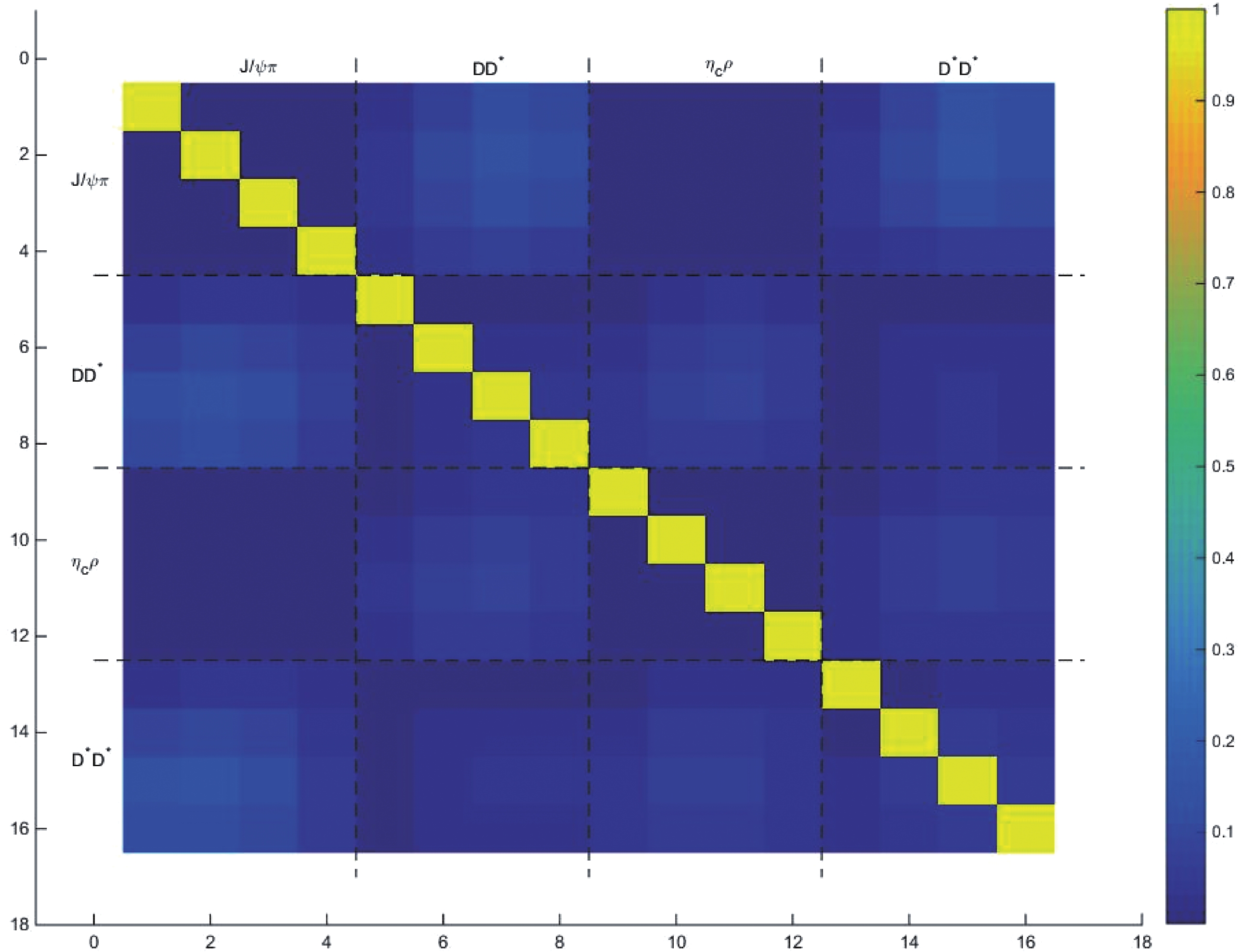
Figure 1. (color online) Density plot of the magnitude of the correlation matrix
$ \tilde{C}_{\alpha\beta}(t) $ as defined in Eq. (51) at$ t = 10 $ obtained from the ensemble. Four channels have been included, each with 4 different back-to-back momentum. It is seen that the coupling between$ J/\psi\pi $ and$ D\bar{D}^* $ is the most important. -
In this paper, we used
$ N_f = 2+1+1 $ twisted mass gauge field configurations generated by the European Twisted Mass Collaboration (ETMC) at$ \beta = 1.9 $ , corresponding to a lattice spacing$ a = 0.0863 $ fm in physical units. Details of the relevant parameters are summarized in Table 1.For the measurements related to the charm sector, we have used the Osterwalder-Seiler type action with a fictitious
$ c' $ quark that is degenerate in c [33].They form an
$ SU(2) $ doublet characterized by a quark mass parameter$ \mu_c $ . The up and down quark mass values are also degenerate and the parameter$ \mu_l $ is fixed to the same value as in the sea corresponding to pion mass$ m_\pi = 320 $ MeV. For the charm quark, the parameter$ \mu_c $ is fixed in such a way that the mass of$ J/\psi $ on the lattice corresponds to$ 2.96 $ GeV. -
We first checked the single meson dispersion relations for the mesons involved:
$ \pi $ ,$ J/\psi $ , D and$ D^* $ . This is crucial since we need well established single meson states in a finite box in order to use the Lüscher formalism. We have attempted to fit the single meson correlators with various momenta using both the continuum and lattice versions of the dispersion relations:$ \begin{split} E^2( { p}) =& m^2+Z_{\mbox{cont.}} { p}^2\;, \\ 4\sinh^2\left(\frac{E( { p})}{2}\right) =& 4\sinh^2\left(\frac{m}{2}\right)+Z_{\mbox{latt.}} \sum^3_{i = 1}4\sin^2\left(\frac{p_i}{2}\right)\;. \end{split} $

(52) It turns out that both work fine for small enough
$ { p}^2 $ , except that the lattice version is better in the sense that the slope$ Z_{\mbox{latt.}} $ is closer to unity than$ Z_{\mbox{cont.}} $ . In Fig. 2, the lattice version of the dispersion relations is illustrated for the above listed mesons. Data points are obtained from the corresponding single-meson correlators, while the lines represent linear fits using Eq. (52).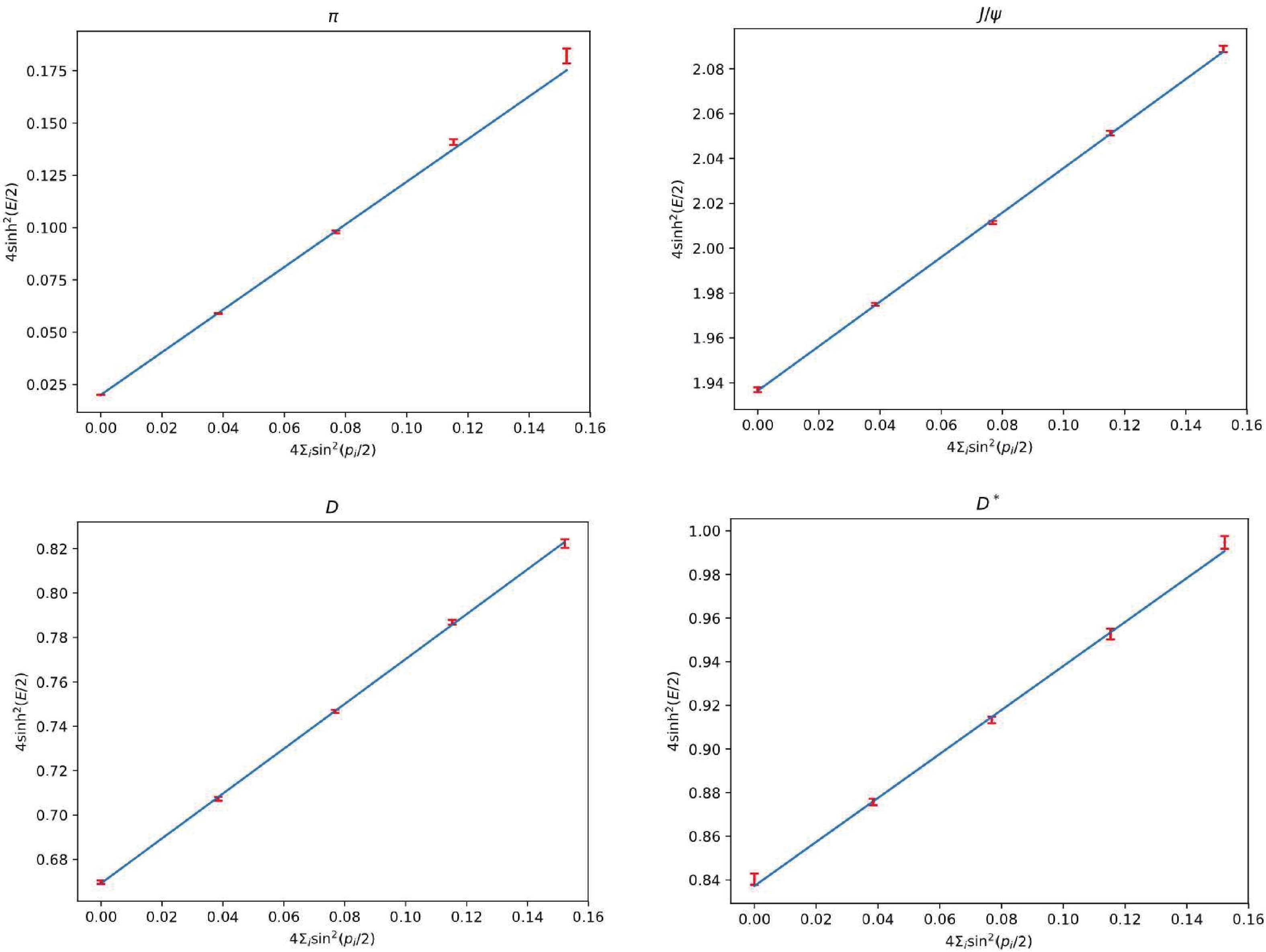
Figure 2. (color online) Single meson dispersion relations (the lattice version) for
$ J/\psi $ ,$ \pi $ , D and$ D^* $ , respectively. Data points are obtained from the corresponding single meson correlators, and the lines are linear fits using Eq. (52). -
To extract the two-particle energy eigenvalues, we adopt the usual Lüscher-Wolff method [9]. For this purpose, a new matrix
$ \Omega(t,t_0) $ is defined as:$ \begin{array}{l} \Omega(t,t_0) = C(t_0)^{-{1\over2}}C(t)C(t_0)^{-{1\over 2}}, \end{array} $

(53) where
$ t_0 $ is the reference time. Normally one chooses$ t_0 $ such that the signal is good and stable. The energy eigenvalues for the two-particle system are then obtained by diagonalizing the matrix$ \Omega(t,t_0) $ . The eigenvalues of the matrix have the usual exponential decay behavior as described by Eq. (50), and therefore the exact energy$ E_\alpha $ can be extracted from the effective mass plateau of the eigenvalue$ \lambda_\alpha $ .Since we are only interested in the two-channel scenario, we focus on the correlation sub-matrix in the
$ J\psi\pi $ and$ D\bar{D}^* $ sector. The correlation matrix is therefore$ 8\times 8 $ , and the GEVP process yields$ 8 $ energy levels. In order to obtain a good plateau for each energy level, we tried to remove the thermal state contamination arising from the lightest$ J/\psi\pi $ state, see e.g. Refs. [31, 34]. In Fig. 3 , we show a typical behavior of one energy eigenvalue plateau both with and without this procedure. It is seen that after performing the thermal state removal procedure, the plateau behavior is greatly improved.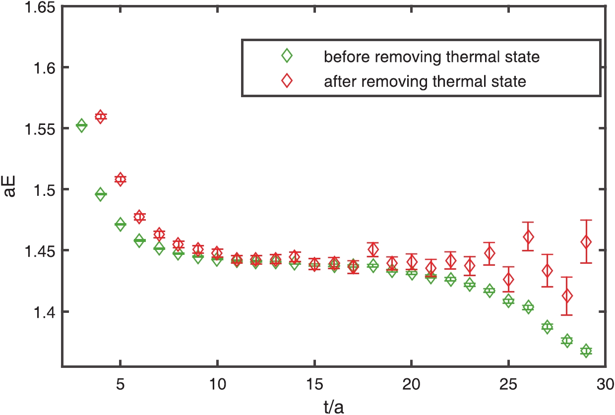
Figure 3. (color online) Effective mass plateau for one of the energy eigenvalues, with and without the thermal state removal.
All effective mass plateaus are shown in Fig. 4, and the final results for
$ E_\alpha $ and the corresponding errors, which are analyzed using the jackknife method, are summarized in Table 2 together with the fitting ranges and$ \chi^2 $ per degree of freedom. It is seen that all energy levels have a suitable plateau behavior.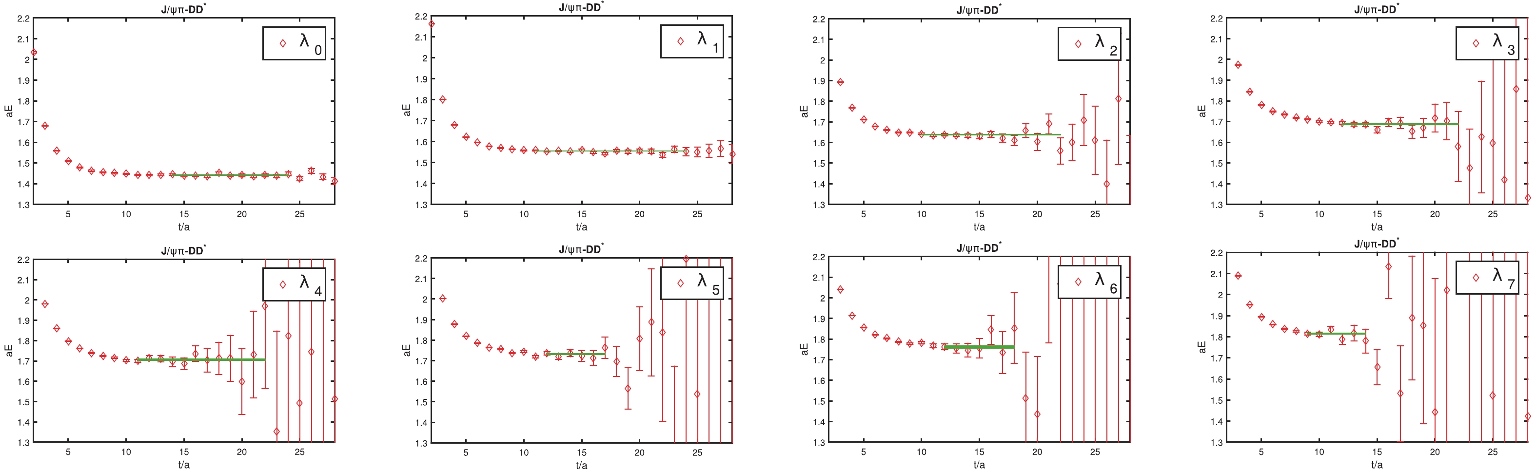
Figure 4. (color online) Effective mass plateaus for the eight energy levels.
Eigenvalues $[t_{\min},t_{\max}]$ 

$E_\alpha$ 

$\chi^2/N_{d.o.f}$ 

$\lambda_0$ 

[14, 24] 1.4411(7) 0.6 $\lambda_1$ 

[11, 24] 1.5547(6) 1.1 $\lambda_2$ 

[10, 22] 1.6375(10) 0.7 $\lambda_3$ 

[12, 22] 1.6868(23) 0.6 $\lambda_4$ 

[11, 22] 1.7058(31) 0.3 $\lambda_5$ 

[12, 18] 1.7319(33) 0.4 $\lambda_6$ 

[12, 18] 1.7610(63) 0.4 $\lambda_7$ 

[9, 14] 1.8152(30) 0.6 Table 2. Energy eigenvalues obtained in the coupled two-channel scattering.
-
As discussed previously, using the Ross-Shaw theory, we adopt a four-parameter fit for the data. To be specific, we use
$ M_{11} $ ,$ M_{12} $ ,$ M_{22} $ and R as the parameters to be determined, assuming that the effective range is the same in the first and second channel. We denote these four parameters as$ \{\lambda_i\} $ , with$ i = 1,2,3,4 $ corresponding to the above listed four parameters.The two-channel Lüscher formula as shown in Eq. (6) can be written as,
$ \begin{array}{l} F(\{\lambda_i\};E) = 0\;, \end{array} $

(54) for an energy level E in the finite box. The function F involves various zeta-functions which can be computed numerically once the parameters are given. Thus, for a given set of parameters
$ \{\lambda_i\} $ , the above formula can be viewed as an equation for E. In fact, one can solve for a tower of E which can be compared with the lattice simulations. Therefore, following e.g. Ref. [34], we may construct a$ \chi^2 $ function as,$ \begin{array}{l} \chi^2(\{\lambda_i\}) = \displaystyle\sum\limits_{\alpha\beta}(E^{\rm sol}_\alpha(\{\lambda_i\})-E^{\rm latt}_\alpha) {\cal C}^{-1}_{\alpha\beta}(E^{\rm sol}_\beta(\{\lambda_i\})-E^{\rm latt}_\beta) \;, \end{array} $

(55) where the summation of
$ \alpha $ and$ \beta $ runs over all available energy levels used in the fit. The energy levels$ E^{\rm sol}_\alpha(\{\lambda_i\}) $ are obtained by solving Eq. (54) once the parameters$ \{\lambda_i\} $ are given. The energy levels$ E^{\rm latt}_\alpha $ correspond to the levels obtained from the lattice data following the GEVP process. The matrix$ {\cal C} $ accounts for the correlation of these quantities since they are all obtained using the same ensemble. We estimated the covariance matrix$ {\cal C} $ from our data using the jackknife method.After minimizing the function can be obtained. In our calculations, we obtained 8 energy levels. Since the highest energy level is subject to contamination, we decided to fit the scattering parameters with and without this level. It turned out that with the highest energy level included, we get a rather large
$ \chi^2 $ , while using the lowest 7 levels yields a tolerable$ \chi^2 $ value. We therefore only list the best fit parameters using the lowest 7 levels. When performing the fit, we used the four parameters including R, and in the zero-range approximation where$ R = 0 $ . It was observed that the four-parameter fit yields a value of R that is consistent with zero within errors. Therefore, it makes sense to perform the fit in the zero-range approximation.The covariance matrix of the fit parameters can be estimated following the standard jackknife procedure. For the case of a three-parameter fit, i.e. in the zero-range approximation, we obtained the inverse covariance matrix
$ C^{-1} $ in lattice units as,$ \begin{array}{l} C^{-1} = \left[ \begin{array}{ccc} 6.49951962 & 4.3268455 &3.24808892 \\ 4.3268455 &12.51156448 & 9.33781593 \\ 3.24808892 & 9.33781593 & 7.4080769 \end{array}\right]\;, \end{array} $

(56) where the column and rows of the matrix are labeled according to
$ (\eta_1,\eta_2,\eta_3) = (M_{11},M_{12},M_{22}) $ . The covariance matrix C itself can be easily obtained. If we wish to transform these matrix elements into units in which$ k_{10} = 1 $ , they have to be either multiplied or divided by the value of$ k^2_{10} $ in lattice units.The results of the fitting procedure are tabulated in Table 3 , where all quantities are in lattice units. The errors of each parameter are equal to the square root of the corresponding matrix element of the covariance matrix C.
No. of levels $M_{11}$ 

$M_{12}$ 

$M_{22}$ 

R $\chi^2/N_{d.o.f}$ 

7 −7.7(1.8) 3.7(1.1) −3.3(2.8) 0.12(1.2) 0.57/3 7 −7.51(0.45) 3.7(1.2) −3.1(1.5) 0.58/4 Table 3. Parameters M11, M22, M12 and R obtained by minimizing the
$\chi^2$ function defined in Eq. (55). All quantities are in lattice units. The corresponding values of the total$\chi^2$ and the number of degrees of freedom are also listed. The errors of various parameters are obtained by the jackknife analysis. -
Since the presence of the effective range parameter R is marginal, in the following discussion we only focus on the case of three parameters. For later convenience, we collectively denote these parameters as
$ \eta = (M_{11},M_{12},M_{22})^T\in\mathbb{R}^3 $ and the value of$ \eta $ which minimizes the$ \chi^2 $ function is denoted as$ \eta^* $ . All parameters are in units of$ k_{10} $ .In a small neighborhood around the best fit value for
$ \eta $ , the function$ \chi^2(\eta) $ can be parametrized as,$ \begin{array}{l} \chi^2(\eta) = \chi^2(\eta^*)+\displaystyle\frac{1}{2}w^T C^{-1}\cdot w \;, \end{array} $

(57) where
$ w = \eta-\eta^* $ , and C is the covariance matrix, which also yields the errors (and the cross-variance) for the fit parameters.The matrix
$ C^{-1} $ is a$ 3\times 3 $ positive-definite symmetric real matrix which can be diagonalized via some rotation matrix R. In fact, setting$ x = R\cdot w $ and requiring that the new matrix$ R^TC^{-1}R $ is diagonal, we have$ \begin{array}{l} R^T\cdot C^{-1} R = \mbox{Diag}(1/\sigma^2_1,1/\sigma^2_2,1/\sigma^2_3) \;. \end{array} $

(58) The confidence level can then be determined by using the change of the
$ \chi^2 $ function relative to its minimum in the parameter space. Denoting$ \begin{array}{l} \Delta\chi^2(\eta) = \chi^2(\eta)-\chi^2(\eta^*)\;, \end{array} $

(59) this quantity is diagonal in terms of the rotated parameters x:
$ \begin{array}{l} \Delta\chi^2(x) = \displaystyle\frac{1}{2}\displaystyle\sum\limits^3_{i = 1}\displaystyle\frac{x^2_i}{\sigma^2_i} \;. \end{array} $

(60) Therefore, for a given value of
$ \Delta\chi^2(x) $ , the above equation becomes a three-dimensional ellipsoid centered at the origin of$ x\in\mathbb{R}^3 $ , with three half-major axes given by:$ \sqrt{2\Delta\chi^2}\sigma_1 $ ,$ \sqrt{2\Delta\chi^2}\sigma_2 $ and$ \sqrt{2\Delta\chi^2}\sigma_3 $ , respectively. In terms of the original variable w, this is a rotated ellipsoid with the rotation characterized by the matrix R which diagonalizes the matrix$ C^{-1} $ .It is known that for the three-parameter
$ \chi^2 $ fit, the$ 1\sigma $ ,$ 2\sigma $ and$ 3\sigma $ contours ⑤ can be determined by requiring that$\Delta\chi^2 = $ 3.53, 8.02, 14.2 , respectively. Thus, denoting$ w = (M_{11}-M^*_{11}, $ $ M_{12}-M^*_{12}, M_{22}-M^*_{22})^T $ , the ellipsoid,$ \begin{array}{l} \Delta\chi^2 = \displaystyle\frac{1} {2} w^T\cdot C^{-1} \cdot w\;, \end{array} $

(61) centered at
$ \eta^* = (M^*_{11}, M^*_{12},M^*_{22}) $ encloses$ 68 $ %,$ 95.4 $ % and$ 99.7 $ % probability for the parameters.On the other hand, the closeness and narrowness conditions given in Eq. (36) yield a parabola and a hyperbola in the
$ \eta_1-\eta_2 $ plane for a given value of$ \eta_3 = M_{22} $ , respectively. We can require that$ R_{\mbox{close}} $ and$ R_{\mbox{narrow}} $ are smaller than some prescribed cut values,$ \begin{array}{l} R_{\rm{narrow}} \leqslant R^{\rm{cut}}_{\rm{narrow}}\;, \;\; R_{\rm{close}} \leqslant R^{\rm{cut}}_{\rm{close}}\;. \end{array} $

(62) We can therefore check whether these conditions are supported by our
$ \chi^2 $ fit.To summarize, these conditions are, using the units system where
$ k_{10} = 1 $ :$ \begin{array}{l} \frac{1}{2}(\eta-\eta^*)^TC^{-1}\cdot (\eta-\eta^*) \leqslant \Delta\chi^2 \;, \end{array} $

(63) $ \begin{array}{l} \eta^2_1- \frac{\displaystyle\eta^2_2}{\displaystyle R^{\rm cut}_{\rm narrow} } \leqslant 1\;, \end{array} $

(64) $ \begin{array}{l} \eta_1[\eta_3+ R^{\rm cut }_{\rm close} ] \leqslant \eta^2_2 \;. \end{array} $

(65) For a given value of
$ \Delta\chi^2 $ , the first inequality (63) imposes an ellipsoid that encloses a certain probability around the best fit value at$ \eta = \eta^* $ ; the second inequality (64) implies a region bounded by a hyperbola in the$ \eta_1\eta_2 $ plane independent of the value of$ \eta_3 = M_{22} $ ; the third inequality requires that the point$ (\eta_1,\eta_2 $ ) is in a region that is above the parabola for a given value of$ \eta_3 = M_{22} $ .Therefore, if we want to have a narrow resonance close enough to the threshold, described by the ratios
$ R^{\rm{cut}}_{\rm{narrow}} $ and$ R^{\rm{cut}}_{\rm{close}} $ , it has to lie in the overlapping region of the above mentioned parabola and hyperbola. By inspecting the location of the overlapping region with respect to$ \Delta\chi^2 $ contours, we can set the confidence intervals for the parameters. This can be done when a particular value of$ \eta_3 = M_{22} $ is given.In Fig. 5, the situation is illustrated for three particular values (from left to right) of
$ M_{22} $ , namely$ M_{22} = M^*_{22}, M^*_{22}+\Delta M_{22}, M^*_{22}-\Delta M_{22} $ , where$ \Delta M_{22} $ is the error of$ M_{22} $ . Here, all quantities are in the units system where$ k_{10} = 1 $ . In each panel of the figure, the common center of the two ellipses corresponds to the minimum of the$ \chi^2 $ function, i.e. the best fit values of$ (\eta^*_1,\eta^*_2) $ for a given value of$ \eta_3 $ . The two elliptical shaded regions around the common center correspond to$ 1\sigma $ (68% probability) and$ 3\sigma $ (99.7% probability) contours for the parameters$ (\eta_1, \eta_2) = (M_{11},M_{12}) $ . The lower left shaded region corresponds to the narrow resonance condition described by the inequality (64), while the upper right shaded region corresponds to the resonance which is close to the threshold, i.e. inequality (65). In this figure, the two ratios have their "true" physical values for$ Z_c(3900) $ , i.e.$ R^{\rm{cut}}_{\rm{close}} = 0.0211 $ and$ R^{\rm{cut}}_{\rm{narrow}} = 0.065 $ . It is clearly seen that the overlapping regions, which are located in the top left corner of each panel, are very far away from the$ 3\sigma $ contours. Therefore, for this set of parameters, it is highly unlikely that the three-parameter Ross-Shaw model can describe a resonance that, as$ Z_c(3900) $ , is both narrow and close to threshold.
Figure 5. (color online) Various contours obtained from Eq. (63) together with the constraints in Eq. (64) and Eq. (65). Three different panels, from left to right, correspond to different values of
$ \eta_3\equiv M_{22} $ :$ M_{22} = M^*_{22} $ ,$ M_{22} = M^*_{22}+\Delta M_{22} $ and$ M_{22} = M^*_{22}-\Delta M_{22} $ , respectively, where$ \Delta M_{22} $ is the error of$ M_{22} $ . In each panel, the central point of the two ellipses corresponds to the best fit value$ (\eta^*_1,\eta^*_2) $ for a given value of$ \eta_3 $ . The two elliptical shaded regions around the central points correspond to$ 1\sigma $ and$ 3\sigma $ contours for the parameters$ (\eta_1, \eta_2) = (M_{11},M_{12}) $ . The lower left shaded region corresponds to the narrow resonance condition described by the inequality (64), while the upper right shaded region corresponds to the resonance which is close to the threshold, i.e. inequality (65). The two ratios have their "true" values for$ Z_c(3900) $ , i.e.$ R^{\rm{cut}}_{\rm{close}} = 0.0211 $ and$ R^{\rm{cut}}_{\rm{narrow}} = 0.065 $ .Since in our simulations we do not have a physical pion mass and a physical charm quark mass, the two ratios and the parameter
$ k_{10} $ could change to have non-real values. However, since the ratios are dimensionless, we do not expect them to change drastically. Similarly, as we saw previously, the value of$ k_{10} $ is also not very different from its physical value. Nevertheless, we take$ R^{\rm{cut}}_{\rm{narrow}} = R^{\rm{cut}}_{\rm{close}} = 0.1 $ and inspect the relation between the overlapping regions and the constant$ \Delta\chi^2 $ contours again. These are shown in Fig. 6. It is seen that even for this set of parameters, the overlapping regions are still far from the$ 3\sigma $ contours, showing that the three-parameter Ross-Shaw model can not explain a narrow resonance close to the resonance described by$ R^{\rm{cut}}_{\rm{narrow}} \!=\! R^{\rm{cut}}_{\rm{close}} \!=\! 0.1 $ .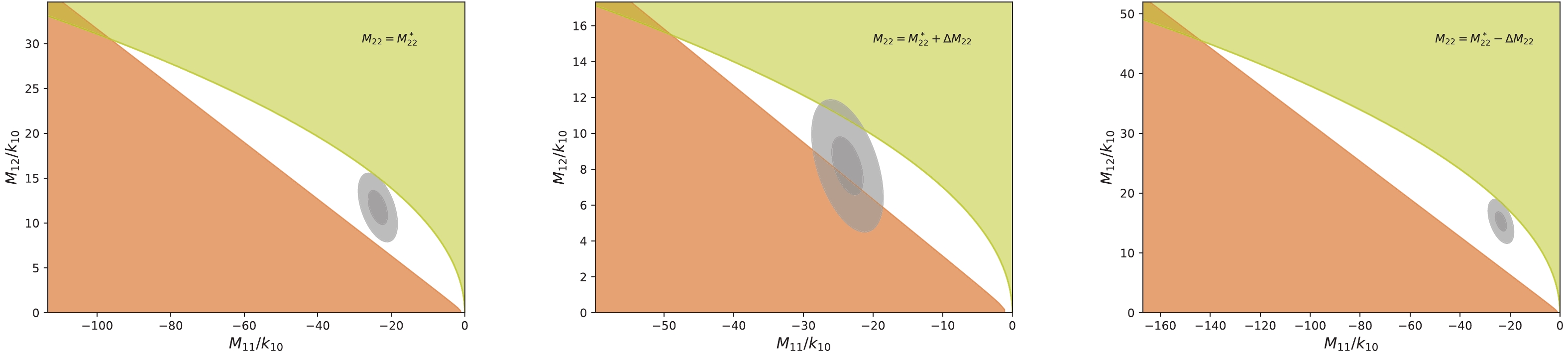
Figure 6. (color online) Same as the previous figure except that the ratios are
$ R^{\rm{cut}}_{\rm{close}} = R^{\rm{cut}}_{\rm{narrow}} = 0.1 $ .We have also tried other parameter sets and the outcome is quite similar. Therefore, as far as the parameters are concerned, it seems that the three-parameter Ross-Show model cannot realize a scenario in which a narrow resonance appears close enough to the threshold. This can be understood from the following physical argument, related to the fact that the best fit values for the M-matrix elements are all very large, either in lattice units or in units of
$ k_{10} $ . Recall that this matrix is related to the$ \cot\delta $ matrix, or to the inverse scattering length matrix, c.f. Eq. (10). Large matrix elements of M, if the matrix itself is non-singular, yield large inverse scattering length, meaning a negligible scattering effect. This is the reason why the zero-range Ross-Shaw theory has difficulty to generate a narrow resonance peak near the threshold. Furthermore, we could ask why are the matrix elements of M so large? This is implicitly hidden in our energy levels$ E_\alpha $ , see Table 2. All energy levels we used in the Lüscher formula are rather close to the free two-particle energy levels. This fact in turn generates large values for the M-matrix elements.However, it is still premature to draw the conclusion that the three-parameter Ross-Shaw theory cannot describe a narrow resonance close to the threshold. In the above argument, we have not taken into account the systematic errors. Only statistical errors are considered and they are assumed to be normally distributed. Although we used dimensionless quantities in our study to bypass the scale setting problems, there are still several systematic effects. Also, we have used one non-physical ensemble, and a further study is required to perform an extrapolation to a physical point. Another systematic effect is that we have only considered two channels. Of course, one could try to add more channels, e.g.
$ \rho\eta_c $ . For that purpose, one needs many more energy levels, since even the three-channel Ross-Shaw theory in the zero-range approximation needs$ 6 $ parameters. In order to determine them, more energy levels are needed, which could be attempted in the future. -
Let us now outline the main conclusions of our study:
● In this exploratory lattice study, we used the coupled-channel Lüscher formula together with the Ross-Shaw theory to study the near-threshold scattering of
$ D\bar{D}^* $ , which is relevant for the exotic state of$ Z_c(3900) $ .● We singled out the two most strongly coupled channels, namely
$ D\bar{D}^* $ and$ J/\psi\pi $ . The fact that these two particular channels show the strongest coupling is supported both by our correlation matrix estimation and by the experimental facts.● Our results showed that the inverse scattering length parameters
$ M_{11} $ ,$ M_{12} $ and$ M_{22} $ are huge in magnitude, indicating that it is unlikely that any resonance that is both narrow and close enough to the threshold could be generated.● Unlike the findings of the HALQCD collaboration, our results do not support a narrow resonance-like peak close to the threshold, when the two most relevant coupled channels are taken into account.
● However, one has to keep in mind that we have not estimated the systematic uncertainties. All error estimates were purely statistical. The systematics could be due to finite lattice spacing, non-physical pion and charm quark masses, finite volume effects, etc., which need to be clarified in future studies.
To summarize, in this paper we presented an exploratory lattice study for the coupled-channel scattering near the
$ D\bar{D}^* $ threshold using the coupled-channel Lüscher formalism. We used the$ 2+1+1 $ twisted mass fermion configurations and a lattice spacing of$ 0.0863 $ fm with the pion mass of$ 320 $ MeV. The two most relevant channels, namely$ J\psi\pi $ and$ D\bar{D}^* $ were studied, which were singled out from the four channels by a correlation matrix analysis. To extract the scattering information, we fitted our lattice results using the Ross-Shaw theory, a multi-channel generalization of the conventional effective range theory. Using our lattice data, the matrix elements of the M-matrix were obtained together with the effective range parameter, which turns out to be marginal.Our results indicate that it is unlikely that both the narrow resonance condition and the condition that the resonance is close enough to the threshold could be satisfied, unless the parameters happen to be in a small corner of our parameter space, far away from the best fit values. It should be kept in mind that we have only considered statistical errors, and that further studies with more lattice spacings and volumes, pion masses and charm quark masses, or even more channels, are needed to quantify the systematic effects. We hope that this exploratory study could shed some light on the multi-channel study of the charmed meson scattering, which is intimately related to
$ Z_c(3900) $ .The authors would like to thank F. K. Guo, U. Meissner, A. Rusetsky, C. Urbach for helpful discussions.
A coupled-channel lattice study of the resonance-like structure Zc(3900)
- Received Date: 2019-07-09
- Available Online: 2019-10-01
Abstract: In this exploratory study, near-threshold scattering of D and


 DownLoad: