Alternative methods for measurement of the global polarization of Λ hyperons

1. Introduction

• 1. Introduction
• 2. Hyperon weak decay and polarization
• 3. STAR method for measurement of the Λ hyperon polarization
• 4. Alternative methods
• 5. Simulation results with UrQMD
• 6. Summary

It is well-known that rotation and polarization are inherently correlated: the rotation of an uncharged object can lead to spontaneous magnetization and polarization, and vice versa [1, 2]. We expect that the same phenomena exist in heavy ion collisions. It is straightforward to estimate the huge global angular momenta that are generated in non-central heavy ion collisions at high energies [3-8]. How such huge global angular momenta are converted to particle polarization in the hot and dense matter, and how can the global polarization be measured, are two core questions to be answered. Several theoretical models are available that address the first question, e.g. the microscopic spin-orbital coupling model [3, 4, 8, 9], the statistical-hydro model [10-13] and the kinetic model with Wigner functions [14-17], see Ref. [18] for a recent review. As for the second question, the weak decay property of Λ hyperons can be used for measurement of the global polarization [3, 4]: the parity-breaking weak decay of Λ into a proton and a pion is self-analyzing since the daughter proton is emitted preferentially along the spin of the Λ in its rest frame [5, 19]. The global polarization of a vector meson can be measured using the angular distribution of its decay products, which is related to the elements of its spin density matrix [4].

Recently, the global polarization of Λ and $\bar{\Lambda }$ hyperons was measured for collision energies below 62.4 GeV [20, 21]. The average values of the global polarization for Λ and $\bar{\Lambda }$ are ${{\mathscr{P}}}_{\Lambda }=(1.08\pm 0.15) \%$ and ${{\mathscr{P}}}_{\bar{\Lambda }}=(1.38\pm 0.30) \%$. The polarization of $\bar{\Lambda }$ is somewhat larger than that of Λ, and is thought to be caused by a negative (positive) magnetic moment of Λ($\bar{\Lambda }$) in magnetic fields. However, the difference is negligible, it is well within the error bars, and the magnetic fields extracted from the data are consistent with zero. The global polarization of Λ and $\bar{\Lambda }$ decreases with collision energy. This is due to the fact that Bjorken scaling works better at higher energies. From the data one can estimate the local vorticity: ω = (9±1) × 10²¹s⁻¹, implying that the matter created in ultra-relativistic heavy ion collisions is the most vortical fluid that exists in nature. The vorticity field of the quark gluon plasma has been studied by many authors using a variety of methods including hydrodynamical models [22-24] and transport models [25, 26]. The global polarization of Λ and $\bar{\Lambda }$ has also been calculated by hydrodynamical models [27, 28], the transport model [29] and the chiral kinetic model [30].

The method used in the STAR experiment is by event averaging of $\sin ({\phi }_{{\rm{p}}}^{* }-{\psi }_{{\rm{RP}}})$, where ${\phi }_{{\rm{p}}}^{* }$ and ψ_RP are the azimuthal angles, in the Λ rest frame, of the proton momentum and of the reaction plane, respectively [20, 21]. The orientation of the reaction plane cannot be directly measured; it is derived from the event plane, itself determined from the direct flow. Therefore, a reaction plane resolution factor was introduced to account for the finite resolution of the reaction plane as given by the detector [20, 21].

In this paper, we propose alternative methods for measurement of the global polarization of Λ and $\bar{\Lambda }$ hyperons based on the Lorentz transformation. The advantage of these methods is that all event averages are taken using momenta in the lab frame instead of the Λ rest frame. We compare these methods by simulations and show that all of them work equally well in obtaining the global polarization of Λ hyperons.

2. Hyperon weak decay and polarization

• 1. Introduction
• 2. Hyperon weak decay and polarization
• 3. STAR method for measurement of the Λ hyperon polarization
• 4. Alternative methods
• 5. Simulation results with UrQMD
• 6. Summary

The polarization of the Λ (and $\bar{\Lambda }$) hyperons can be measured by its parity-breaking weak decay Λ→p+π⁻. The daughter proton is emitted preferentially along the Λ polarization in its rest frame. The angular distribution of the daughter proton reads

where α_H is the hyperon decay parameter, $\begin{eqnarray}{{\mathscr{P}}}_{\Lambda}\end{eqnarray}$ is the Λ global polarization; n^*, p^* and Ω* are the Λ polarization, the proton momentum and its solid angle in the rest frame of the hyperon, respectively, labeled by the superscript ′*′. We note that Eq. (1) is Lorentz invariant by observing

where p^μ and ${p}_{\Lambda }^{\mu }$ are the four-momenta of the proton and the hyperon in any frame, respectively, and n^μ is the space-like four-vector of the hyperon polarization in a general frame. We now focus on the lab frame and the hyperon rest frame. We use p^μ, ${p}_{\Lambda }^{\mu }$ and n^μ to label quantities in the lab frame; all quantities with the superscript ′*′ are in the hyperon rest frame. The Lorentz transformation of the Λ polarization is,

where ${\Lambda }_{\, \nu }^{\mu }(-{\mathit{\boldsymbol{v}}}_{\Lambda })$ is the Lorentz transformation with ${\mathit{\boldsymbol{v}}}_{\Lambda }={\mathit{\boldsymbol{p}}}_{\Lambda }/{E}_{\Lambda }$. The Λ polarization in the rest frame n^*ν has the form n^*μ = (0, n^*) where n^* is the three-vector of the polarization with |n^*|² <1. From Eq. (3) we have

We can also express n^*μ in terms of n^μ,

or explicitly,

The polarization four-vector of a particle is always orthogonal to its four-momentum, n·p_Λ = n⁰E_Λ-n·p_Λ=0, so we can express n⁰ in term of n, n⁰ = n·v_Λ. One can verify that n^μ in Eq. (4) satisfies n⁰=n·v_Λ. From (n⁰)²-|n|² = -|n^*|² and n⁰=n·v_Λ, we can solve for |n|² giving

We see that when $|{\mathit{\boldsymbol{v}}}_{\Lambda }{|}^{2}{(\hat{\mathit{\boldsymbol{n}}}\cdot {\hat{\mathit{\boldsymbol{v}}}}_{\Lambda })}^{2}\to 1$, |n|²→∞, i.e. |n|² is not bounded. In case of transverse polarization, i.e. $\hat{\mathit{\boldsymbol{n}}}\cdot {\hat{\mathit{\boldsymbol{v}}}}_{\Lambda }=0$, we have |n|² = |n^*|² < 1.

In the lab frame, a 3-dimensional vector (e.g. impact parameter, global angular momentum, beam direction) can be written as a = a_xe_x+a_ye_y+a_ze_z, where (e_x, e_y, e_z) are the three basis directions.

3. STAR method for measurement of the Λ hyperon polarization

• 1. Introduction
• 2. Hyperon weak decay and polarization
• 3. STAR method for measurement of the Λ hyperon polarization
• 4. Alternative methods
• 5. Simulation results with UrQMD
• 6. Summary

In this section we describe briefly the method used in the STAR experiment for measurement of the Λ hyperon polarization [21]. From Eq. (13), we can determine the Λ polarization in its rest frame by taking the event average of the direction of the proton momentum ${\hat{\mathit{\boldsymbol{p}}}}^{* }$. We then make a projection onto the direction of the global angular momentum e_L,

where θ^* is the angle, in the Λ rest frame, between the proton momentum and the global angular momentum corresponding to the reaction plane. We have the following relation

where ${\theta }_{{\rm{p}}}^{* }$ and ${\phi }_{{\rm{p}}}^{* }$ are the polar and azimuthal angles of ${\hat{\mathit{\boldsymbol{p}}}}^{* }$, respectively, and ψ_RP is the azimuthal angle of the reaction plane. We integrate over ${\theta }_{{\rm{p}}}^{* }$ in Eq. (1) to obtain

which gives the polarization in terms of the azimuthal angle of the daughter proton,

with

In the STAR experiment, the azimuthal angle of the reaction plane cannot be directly measured. It is determined from the measurement of the event plane given by the direct flow. This introduces a reaction plane resolution factor in the denominator of Eq. (11), ${R}_{{\rm{EP}}}^{(1)}={\langle \cos ({\psi }_{{\rm{RP}}}-{\psi }_{{\rm{EP}}}^{(1)})\rangle }_{{\rm{ev}}}$, where ${\psi }_{{\rm{EP}}}^{(1)}$ is the azimuthal angle of the event plane determined by the direct flow.

4. Alternative methods

• 1. Introduction
• 2. Hyperon weak decay and polarization
• 3. STAR method for measurement of the Λ hyperon polarization
• 4. Alternative methods
• 5. Simulation results with UrQMD
• 6. Summary

In this section, we introduce alternative methods for measurement of the Λ hyperon polarization. The advantage of these methods is that the polarization can be measured using the proton momentum in the lab frame.

We start with the formula for the Λ polarization vector in its rest frame,

We can project the above onto the direction of the global polarization, which we assume to be along the y-axis, see Fig. (1).

We now try to evaluate ${\langle {\hat{\mathit{\boldsymbol{P}}}}^{* }\rangle }_{{\rm{ev}}}$. To this end, we use the following Lorentz transformation of the proton momentum,

where ${E}_{{\rm{p}}}^{* }$ is determined by the masses of the proton, pion and Λ, as in Eq. (2). We take the event average of 〈p〉_ev,

where we have used 〈p_Λ〉_ev = 0.

In order to evaluate the second event average in the right-hand-side of Eq. (15), we make two assumptions: (1) p_Λ and p^* are statistically independent, so we have ${\langle \mathit{\boldsymbol{p}}_{\Lambda }(\mathit{\boldsymbol{p}}_{\Lambda }\cdot \mathit{\boldsymbol{p}}^{* })\rangle }_{{\rm{ev}}}\approx \mathit{\boldsymbol{e}}_{i}{\langle \mathit{\boldsymbol{p}}_{\Lambda }^{i}\mathit{\boldsymbol{p}}_{\Lambda }^{j}\rangle }_{{\rm{ev}}}{\langle \mathit{\boldsymbol{p}}_{j}^{* }\rangle }_{{\rm{ev}}}$, where $\mathit{\boldsymbol{p}}_{\Lambda }=\mathit{\boldsymbol{e}}_{i}\mathit{\boldsymbol{p}}_{\Lambda }^{i}$ with i = x, y, z; and (2) ${\langle \mathit{\boldsymbol{p}}_{\Lambda }^{i}\mathit{\boldsymbol{p}}_{\Lambda }^{j}\rangle }_{{\rm{ev}}}={\langle |\mathit{\boldsymbol{p}}_{\Lambda }^{i}{|}^{2}\rangle }_{{\rm{ev}}}{\delta }_{ij}$. Eq. (15) then becomes

We choose a coordinate system as in Fig. 1: the impact parameter vector is along the x-axis, the global orbital momentum is along the y-axis, and the beam direction is along the negative z-axis. In the coordinate system used in the experiment, the beam direction is along the negative z-axis, and the impact parameter vector (reaction plane) is at an azimuthal angle ψ_RP relative to the x-axis. In the new coordinate system, we have $\mathit{\boldsymbol{p}}_{\Lambda, {\rm{p}}}^{x}=|\mathit{\boldsymbol{p}}_{\Lambda, {\rm{p}}}^{T}|\cos ({\phi }_{\Lambda, {\rm{p}}}-{\psi }_{{\rm{RP}}})$ and $\mathit{\boldsymbol{p}}_{\Lambda, {\rm{p}}}^{y}=|\mathit{\boldsymbol{p}}_{\Lambda, {\rm{p}}}^{T}|\sin ({\phi }_{\Lambda, {\rm{p}}}-{\psi }_{{\rm{RP}}})$, where ϕ_{Λ, p} are the azimuthal angles of the Λ hyperon and proton, respectively.

Figure 1

Figure 1.  (color online) In the coordinate system (x, y, z), the beam direction is along the negative z-direction, the impact parameter vector is in the x-direction, and the orbital angular momentum is in the y-direction. The direction of the proton momentum can be described by the polar angle θ_p and the azimuthal angle ϕ_p. The coordinate system (x′, y′, z′) is used in experiment. The z′-axis is just the z-axis. The azimuthal angle of the impact parameter vector in the (x′, y′, z′) system is ψ_RP.

DownLoad: Full-Size Img PowerPoint

We can further simplify Eq. (16) by using the elliptic flow coefficients. The distribution of p_Λ is not isotropic but satisfies

where ${v}_{2}^{\Lambda }$ is the elliptic flow of the Λ hyperon. Since the global angular momentum is along the y-axis, we have 〈p_x〉_ev = 〈p_z〉_ev = 0, and the only non-vanishing component is

In the central rapidity region $|\mathit{\boldsymbol{p}}_{\Lambda }^{z}|\ll |\mathit{\boldsymbol{p}}_{\Lambda }^{T}|$ and $|\mathit{\boldsymbol{p}}_{\Lambda }^{T}|\approx |\mathit{\boldsymbol{p}}_{\Lambda }|$, so that Eq. (18) becomes

In the non-relativistic limit, γ_Λ ≈ 1 and |v_Λ| ≈ 0, we obtain

The difference with respect to the STAR method is that now we are taking the event average using the proton momenta in the lab frame.

Another method is to use the Lorentz transformation of the energy associated with Eq. (14)

to replace (p^*·p_Λ)/m_Λ with ${E}_{{\rm{p}}}-{\gamma }_{\Lambda }{E}_{{\rm{p}}}^{* }$. Eq. (14) then becomes

Taking the event average and using 〈p_Λ/(E_Λ+m_Λ)〉 ≈ 0, we obtain

where γ_p and γ_Λ are Lorentz contraction factors for the proton and Λ hyperon, respectively. The right-hand-side of the above equation involves only momenta in the lab frame. We can project Eq. (23) onto the y-direction (the direction of the orbital angular momentum) to obtain ${\langle {\mathit{\boldsymbol{p}}}_{y}^{* }\rangle }_{{\rm{ev}}}$.

With ${\langle {\hat{\mathit{\boldsymbol{p}}}}_{y}^{* }\rangle }_{{\rm{ev}}}$ given by one of Eqs. (18, 19, 23), we can obtain the global polarization of Λ from Eq. (13). In the next section we compare these methods by simulations.

5. Simulation results with UrQMD

• 1. Introduction
• 2. Hyperon weak decay and polarization
• 3. STAR method for measurement of the Λ hyperon polarization
• 4. Alternative methods
• 5. Simulation results with UrQMD
• 6. Summary

The UrQMD model [31, 32] has been used to produce an ensemble of Λ hyperon four-momenta (E_Λ, p_Λ) from Au+Au collisions with an impact parameter of 6 fm and collision energies listed in Table 1. In each event there are a few Λ hyperons produced. All these hyperons are collected. Each hyperon is allowed to decay into a proton and a pion, whose angular distribution in the Λ rest frame is given by

Table 1

Table 1.  Simulation results for the global polarization of Λ hyperons. We set ${{\mathscr{P}}}_{\Lambda }=1/3$, i.e. the Λ hyperons are completely polarized. By analyzing the momentum distribution of daughter protons in the lab frame, we determine the Λ polarization. The results of five methods are presented: methods 1 and 2, Eqs. (8, 11) are used in the STAR experiment [21]; methods 3-5, given by Eqs. (18, 23, 19) are proposed in this paper. The number of events collected are 4 × 10⁴ at 200 GeV and 2.5 × 10⁴ at other energies. The results of method 1-4 are from events in the full rapidity range, while those of method 5 are in the rapidity range [−0.5, 0.5]

energy/GeV	method 1 Eq. (8)	method 2 Eq. (11)	method 3 Eq. (18)	method 4 Eq. (23)	method 5 Eq. (19)	number of Λs (full rapidity)
200	0.33581	0.335851	0.3324	0.33014	0.308495	1304795
180	0.330877	0.33141	0.326565	0.329057	0.306966	927717
140	0.338745	0.337673	0.338942	0.335862	0.351934	892533
120	0.333962	0.333688	0.329696	0.334152	0.318965	995522
100	0.336686	0.334685	0.34669	0.34522	0.360992	971596
62.4	0.331964	0.33118	0.324133	0.333466	0.353216	918787
40	0.330536	0.330302	0.332092	0.331782	0.323459	795837
39	0.337252	0.337516	0.332983	0.331683	0.312195	847367
19.6	0.328531	0.328434	0.339587	0.328939	0.31276	707868
7.7	0.341257	0.3417	0.364069	0.34862	0.302301	434697

DownLoad: CSV

Show Table

where ${{\mathscr{P}}}_{\Lambda }$ denotes the Λ polarization. By taking a specific value of ${{\mathscr{P}}}_{\Lambda }$, we sample proton momenta in Λ rest frames. For each Λ hyperon, the proton momentum in its rest frame is then boosted back to the lab frame. In this way we create an ensemble of proton momenta in the lab frame. With the ensemble of momenta for protons and Λ hyperons, we obtain ${\langle \mathit{\boldsymbol{p}}_{y}^{* }\rangle }_{{\rm{ev}}}$. Here we choose the direction of the global angular momentum along the y-direction. Finally, we obtain ${\langle {p}_{y}^{* }\rangle }_{{\rm{ev}}}$ from Eq. (13). Simulation results for the global polarization of Λ hyperons using the methods given by Eqs. (8, 11, 18, 23, 19) are shown in Table 1. We see that all proposed methods give equivalent results to the STAR method. Fig. 2 shows the dependence of the simulation results on the rapidity ranges. We conclude that all methods work well for the chosen rapidity ranges, except method Eq. (19) when used in the full rapidity range, or in ranges [−1.5, 1.5] and [−1, 1]. This is understandable since Eq. (19) is only valid for central rapidity. When applied in the rapidity range [−0.5, 0.5], this method also works well.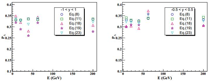

Figure 2

Figure 2.  (color online) The dependence of simulation results on rapidity ranges for the global polarization of the Λ hyperon. The same parameters and number of events are used as in Table 1.

DownLoad: Full-Size Img PowerPoint

6. Summary

• 1. Introduction
• 2. Hyperon weak decay and polarization
• 3. STAR method for measurement of the Λ hyperon polarization
• 4. Alternative methods
• 5. Simulation results with UrQMD
• 6. Summary

The method used in the STAR experiment for measurement of the global polarization of Λ hyperons is by event averaging of $\sin ({\phi }_{{\rm{p}}}^{* }-{\psi }_{{\rm{RP}}})$, where ${\phi }_{{\rm{p}}}^{* }$ and ψ_RP are the azimuthal angles of the proton momentum in the Λ rest frame and of the reaction plane, respectively. We propose several alternative methods for measurement of the Λ global polarization. Based on the Lorentz transformation of momenta, we express the global polarization in terms of momenta of protons and Λ hyperons in the lab frame, and the event average is then taken of relevant quantities in this frame. To test these methods, we used the UrQMD model to produce an ensemble of Λ hyperon momenta and then sampled the angular distribution of protons and pions following the weak decay of Λ hyperons. By taking event averages of relevant quantities as function of momenta of protons and Λ hyperons in the lab frame, we determined the global polarization. The simulations showed that all proposed methods work equally well as the STAR method.

References