


 Abstract
 HTML
HTML Reference
 Related
 PDF
PDF


-
Investigations on stellar astrophysical compact objects (
${\rm COs}$ ) according to the basic formulation of the general theory of relativity (GR) constitute a growing and interesting field of research. Notably, the modeling of such gravitational${\rm COs}$ requires that they be static or non-static and spherically symmetric to observe their stable configurations. Accordingly, among theorists and astrophysicists, the development of a realistic and potentially stable model of an astrophysical$ {\rm CO} $ , together with the distribution of an electric charge, is important. To realize the foregoing, it is necessary to simplify the system of the Einstein-Maxwell field equations into a less complex system by adopting a better mathematical tool. Accordingly, numerous researchers have chosen distinctive ansatzes to comprehend these equations, and several authors such as Patel and Kopper [1], Patel et al. [2], Tikekar and Singh [3], Sharma et al. [4], and Komathiraj and Maharaj [5] have used various numerical strategies to obtain definite solutions for relativistic${\rm COs}$ . These investigations have demonstrated that the system of field equations is adequate to describe astrophysical${\rm COs}$ .In the
${\rm GR}$ , exact solutions are physically viable and robustly utilized in numerous applications of astrophysical${\rm COs}$ . Notably, obtaining the analytical solutions to the Einstein-Maxwell equations is one of the basic problems in the${\rm GR}$ , as well as among the modified versions of this theory of gravitation. Because it is crucial to guarantee the validity of the physical nature of these solutions, the physical effectiveness of the exact solutions was tested by Delgaty and Lake [6]. Consequently, these authors established geometrical standards for the gravitational potential, which imperatively satisfy all the physical traits.The presence of an electric charge within the matter content creates an extraordinary theoretical interest toward the electromagnetic effects on stellar astrophysical
${\rm COs}$ . Gupta and Maurya [7, 8] developed super-dense star models in the presence of electric intensity. Consequently, they discovered that the obtained solutions were well-behaved and regular within the entire domain of the star. Maurya and Gupta [9] proposed certain vital features of charged objects by assigning the value of an electric parameter. Pant et al. [10] explored various solutions to the charged matter influence with a finite pressure and matter density that satisfied the casuality condition$\Big(\dfrac{{\rm d} P_{r}}{{\rm d} \rho}\leq 1\Big)$ and exhibited a positive nature at the center. Further, some well-behaved charged${\rm COs}$ were investigated by Maurya and Gupta [11, 12] with a metric potential$ g_{44}=B (1+ C r^{2})^{n} $ . In addition to the previously mentioned studies, several researchers [11–14] have contributed a variety of novel solutions pertaining to the modeling of charged${\rm COs}$ .In recent decades, numerous authors have obtained exact solutions to the Einstein-Maxwell field equations for an isotropic fluid. Further, some global and physically realistic solutions of a charged isotropic fluid and the Reissner-Nordstr
$ \ddot{o} $ m metric have been investigated by Ivanov [15]. However, to obtain the exact solution, one must integrate the Einstein-Maxwell field equations. Therefore, distinctive confinements have been set by researchers on the spacetime geometry, as well as on the matter distribution. Under the supposition of a constant hypersurface, Komathiraj and Maharaj [16] introduced charged spherical models. By setting a constraint on the gravitational potential, Thirukkanesh and Maharaj [17] and Komathiraj and Maharaj [5] investigated the exact solutions to the Einstein-Maxwell field equations in the presence of isotropic matter. Mak and Harko [18] proposed different techniques to evaluate various physical aspects of isotropic spheres. However, several researchers have revealed that pressure anisotropy is an underlying ingredient of the modeling of${\rm COs}$ . The modeling of anisotropic${\rm COs}$ is an extensive and vast dynamical field that has attracted great attention from researchers over the last several decades. For example, Ruderman [19] provided the basic foundation for the configuration of stellar anisotropic${\rm COs}$ and concluded that the extreme dense regions of${\rm COs}$ contain an anisotropic fluid. Further, Bowers and Liang [20] studied the possible causes of anisotropic stress. Subsequently, the impacts of anisotropic pressure on the system of a general relativistic sphere and its physical characteristics were investigated by Dev and Gleiser [21, 22]. Herrera et al. [23–28] considered a class of exact solutions to a set of field equations regarding the physical emergence of anisotropic pressure in self-gravitating structures. Moreover, Fuloria and Pant [29] and Maurya and Maharaj [30] suggested various types of analytical solutions to demonstrate the physical implications of anisotropic compact spheres in the regime of the Karmarkar approach. Additionally, certain classes of exact relativistic solutions to the Einstein field equations for anisotropic spherically symmetric and static dense compact star models, inspired by the Buchdahl and Korkina-Orlyanskii ansatzes, have been proposed in Refs. [31–34]. Recently, several researchers have made phenomenological considerations in the assessments of the physical influence of anisotropic stress within the realm of the${\rm GR}$ , as well as alternative gravitational theories [35–53].Generally, identifying a suitable equation of state (
${\rm EoS}$ ) for the demonstration of astrophysical${\rm COs}$ is fundamental. For instance, Varela et al. [54] discussed the physical reliability of an${\rm EoS}$ in the demonstration of${\rm COs}$ . Sharma and Maharaj [55], Thirukkanesh and Maharaj [56], and Takisa and Maharaj [57] employed a linear${\rm EoS}$ to develop models of dense${\rm COs}$ . For spherically symmetric systems, Hansraj and Maharaj [58] studied the isotropic matter distribution that satisfied the barotropic${\rm EoS}$ , i.e.,$ p_{r}=p_{r}(\rho) $ . For a quadratic${\rm EoS}$ , Feroze and Siddique [59] and Maharaj and Takisa [60] explored the physical implications of charged anisotropic relativistic star models. In the composition of astronomical compact star models, the polytropic${\rm EoS}$ plays a vital role in explaining the various features of compact stars. Chandrasekhar [61] discussed the outcomes of the Newtonian polytropic theory in the context of thermodynamical laws. Herrera and Barreto [62] organized a detailed study of Newtonian polytropic models for an anisotropic fluid. Thirukkanesh and Ragel [63,64] depicted the realistic features of uncharged compact star models in the regime of a polytropic${\rm EoS}$ . Furthermore, Takisa and Maharaj [65] reviewed the physical consequences of a polytropic${\rm EoS}$ on charged anisotropic compact star models. Nilsson and Ugla [66] adopted a standard procedure to obtain a set of equations by considering a polytropic${\rm EoS}$ . Note that this${\rm EoS}$ can be assessed numerically to obtain a finite radius for various values of the polytropic index η ranging from$ 0 $ to 3.339 and to obtain an infinite radius for$ \eta\geq5 $ .The combination of linear and polytropic
${\rm EoS}$ produces the generalized form of a polytropic${\rm EoS}$ , i.e.,$ P_{r}=\alpha \rho + \beta \rho^{1+1/\eta} $ . Several authors have employed the generalized polytropic${\rm EoS}$ to study the definite stellar features of COs; these authors include Chavanis [67] who constructed models of the early and late universe with the generalized polytropic${\rm EoS}$ and concluded that the models were in fine symmetric tune during the early and late epoch of inflation. Azam et al. [68] formulated the general framework to explore the behavior and reliability of Newtonian and relativistic polytropes for the generalized polytropic${\rm EoS}$ . Nasim and Azam [69] proposed physically viable charged anisotropic models by considering the generalized polytropic EoS. To model an ultra relativistic CO, Finch and Skea [70] developed their analytical study against the background of the Duorah and Ray ansatz. Considering the Finch-Skea ansatz, some viable implications for charged anisotropic compact star models were proposed by Hansraj and Maharaj [58] by employing a barotropic$\rm EoS $ . Sharma and Ratanpal [71] reviewed the various useful outcomes of static and spherically symmetric objects in the framework of the Finch-Skea ansatz. Pandya et al. [72] demonstrated generalized results of the Finch-Skea geometry for the modeling of strange quark stars by considering the Chaplygin gas EoS. Recently, several notable characteristics of astrophysical COs have been revealed by assuming the Finch-Skea geometries in various gravitational theories [73–77].This remainder of this manuscript is outlined as follows: In Sec. II, we investigate an equivalent set of Einstein-Maxwell field equations for models of anisotropic astrophysical COs by implementing the generalized polytropic EoS with the transformation introduced by Durgapal and Bannerji [78]. The smooth matching conditions between the interior metric and exterior Reissner-Nordstr
$ \ddot{\ddot{\rm o}} $ m solution at the hypersurface are also investigated. In Sec. III, we assume a gravitational potential Z as the Finch-Skea ansatz, leading to a restricted system of field equations in a comprehensive manner. We obtain various feasible classes of charged polytropic models corresponding to particular choices of the polytropic index η in Sec. IV. Sec. V deals with the physical adequacy of the presented models in evaluating various attributes such as the material quantities, effective mass function, anisotropy, electric charge, and causality condition. The last section includes a summary of our findings. -
We selected a static and spherically symmetric relativistic stellar interior model in the standard coordinate system
$ x^{a}=(x^{1}, x^{2}, x^{3}, x^{4})=(t, r, \theta, \phi) $ , which has the form$ \begin{array}{*{20}{l}} {\rm d}s^2=-{\rm e}^{2\lambda(r)}{\rm d}t^2+{\rm e}^{2\psi(r)}{\rm d}r^{2}+r^{2}{\rm d}\Omega^2, \end{array} $

(1) where
$ \lambda(r) $ and$ \psi(r) $ denote metric potentials for a static gravitational field, and${\rm d}\Omega^{2}={\rm d}\theta^{2}+\sin\theta^{2} {\rm d}\phi^2$ . We assume that the interior region of the stellar model is filled by charged anisotropic matter, and the corresponding total energy-momentum tensor is given by$ T_{a}^{b}={\rm diag} \Bigg[-\rho-\frac{\mathcal{E}^{2}}{2}, P_{r}-\frac{\mathcal{E}^{2}}{2}, P_{t}+\frac{\mathcal{E}^{2}}{2}, P_{t}+\frac{\mathcal{E}^{2}}{2}\Bigg]. $

(2) Here, ρ denotes the energy density.
$ P_{r} $ and$ P_{t} $ correspond to the radial and tangential pressures, respectively.$ \mathcal{E} $ is the electric field intensity. For a static interior compact sphere (1) and anisotropic energy-momentum tensor (2), the Einstein-Maxwell field equations have the following forms:$ 8 \pi \ \rho+\mathcal{E}^{2}=\frac{1}{r^2}\ \Big[r(1-{\rm e}^{-2\psi})\Big]' , $

(3) $ 8 \pi \ P_{r}-\mathcal{E}^{2}=-\frac{1}{r^2}\ \Big(1- {\rm e}^{-2\psi}\Big)+\frac{2\lambda'}{r}{\rm e}^{-2\psi} , $

(4) $ 8 \pi \ P_{t}+ \mathcal{E}^{2}={\rm e}^{-2\psi}\ \Big(\lambda''+\lambda'^{2}+\frac{\lambda'}{r}-\lambda' \psi'-\frac{\psi'}{r}\Big), $

(5) $ \sigma=\frac{1}{r^2}\ {\rm e}^{-\psi}\ \Big(r^2\ \mathcal{E}\Big)'. $

(6) Here, we use the following geometric unit:
$ G = c = 1 $ . The$ ' $ and$ '' $ signs denote the first- and second-order derivatives with respect to r, respectively. The underlying equations describing the fundamental stellar interior model for a charged anisotropic fluid sphere are provided in Eqs. (3)–(6). These Einstein-Maxwell field equations constitute a system of four independent equations with six independent unknowns (λ, ψ, ρ,$ P_{r} $ ,$ P_{t} $ ,$ \mathcal{E} $ , or σ). Notably, if we assume a specific form of the electric field intensity$ \mathcal{E} $ , the system described in Eqs. (3)–(6) becomes a system of three independent equations with five independent unknowns. A charged solution can then be generated by specifying the forms of two unknown functions or each combination of unknown functions and EoSs associated with the matter quantities. To obtain the simplest system, we consider an important relation between the energy density and radial pressure, which is described by the generalized polytropic EoS.$ \begin{array}{*{20}{l}} P_{r}=\mathcal{A}\ \rho+\mathcal{B}\ \rho^{\Gamma}, \end{array} $

(7) where
$ \Gamma= 1+\dfrac{1}{\eta} $ ; here, η refers to the polytropic index.$ \mathcal{A} $ and$ \mathcal{B} $ are arbitrary constants. In decidingcriterions for a certain EoS to construct a stellar relativistic astrophysical CO, rather than the self-gravitating compact model, the radial pressure$ P_{r} $ should be non-negative and regular (finite) at every point inside the star, and it should vanish at the surface$ r=r_{b} $ of the sphere [79]. Therefore, when the pressure is zero at the boundary, it is implied that the density also vanishes on the surface of the star. To obtain a concise system of the field equations, we employ the transformation priory proposed by Durgapal and Banerji [78], which is given as follows$ \begin{array}{*{20}{l}} x=r^{2},\ \ \ \mathcal{Z}(x)= {\rm e}^{-2\psi(r)},\ \ \ y^{2}(x)= {\rm e}^{2\lambda(r)}. \end{array} $

(8) Using the above transformation, Eqs. (3)–(6), along with the generalized polytropic EoS, can be rewritten as
$ 8 \pi\rho=\frac{1}{x}(1-\mathcal{Z})-2\dot{\mathcal{Z}}-\mathcal{E}^{2}, $

(9) $ P_{t}=P_{r}+\Delta , $

(10) $ P_{r}=\mathcal{A}\ \rho + \mathcal{B}\ \rho^{1+\frac{1}{\eta}} , $

(11) $ 8 \pi P_{r}=4\mathcal{Z}\frac{\dot{y}}{y}+\frac{1}{x}\Big(\mathcal{Z}-1\Big)+\mathcal{E}^{2} , $

(12) $ 8 \pi P_{t}=4x\mathcal{Z}\frac{\ddot{y}}{y} +\Big(4\mathcal{Z}+2x\dot{\mathcal{Z}}\Big)\frac{\dot{y}}{y}+\dot{\mathcal{Z}}-\mathcal{E}^{2} , $

(13) $ 8\pi\Delta=4x\mathcal{Z}\frac{\ddot{y}}{y}+2x\frac{\dot{y}}{y}\dot{\mathcal{Z}}+\dot{\mathcal{Z}}+\frac{1}{x}\Big(1-\mathcal{Z}\Big)-2\mathcal{E}^{2} , $

(14) $ \sigma^{2}=\frac{4\mathcal{Z}}{x}\Big(\mathcal{E}+\dot{\mathcal{E}}x\Big)^{2} . $

(15) From Eqs. (7)–(9), we obtain the following:
$ \begin{aligned}[b] \frac{\dot{y}}{y}=&\frac{\mathcal{A}}{4\mathcal{Z}}\Bigg(\frac{1-\mathcal{Z}}{x}-2\dot{\mathcal{Z}}-\mathcal{E}^{2}\Bigg)\\&+\frac{\mathcal{B}(8\pi)^{-\tfrac{1}{\eta}}} {4\mathcal{Z}}\Bigg(\frac{1-\mathcal{Z}}{x}-2\dot{\mathcal{Z}}-\mathcal{E}^{2}\Bigg)^{1+\tfrac{1}{\eta}}+\frac{1-\mathcal{Z}}{4\mathcal{Z}x}-\frac{\mathcal{E}^{2}}{4\mathcal{Z}}, \end{aligned} $

(16) where topmark · represents differentiation with respect to x, and the anisotropy factor is Δ, which reflects the difference between the radial and tangential pressures. In this description, Thirukkanesh and Maharaj [56] used a linear EoS to develop an analogous equatorial system for the modeling of an anisotropic dense compact sphere. Feroze and Siddique [59] and Maharaj and Takisa [60] employed a quadratic EoS to obtain physically realistic compact star models. Furthermore, a polytropic EoS was used by Takisa and Maharaj [57] to construct a charged anisotropic compact star model. Note that the gravitating mass within a sphere of radius r is expressed as
$ M(r)=4\pi \int^r_0 \omega^2 \rho(\omega) {\rm d}\omega. $

(17) The mass function obtained after implementing the transformation assumes the following form:
$ M(x)=2\pi\int^x_0 \sqrt{\omega}\rho(\omega){\rm d}\omega. $

(18) -
Matching conditions are generally employed to connect the interior and exterior geometries of a star at the boundary surface
$ r=r_{b} $ . The choice of the exterior region entirely depends on the interior matter distribution of the star. For a spheroidal structure, if the fluid in the interior of an object is electrically charged and anisotropic, we assume the Reissner-Nordstr$ \ddot{\ddot{o}} $ m metric as the exterior region:$ \begin{aligned}[b] {\rm d}s^2=&-\Bigg(1-\frac{2\tilde{M}}{r_{b}}+\frac{Q^2}{r_{b}^{2}}\Bigg){\rm d}t^2+\Bigg(1-\frac{2\tilde{M}}{r_{b}}+\frac{Q^2}{r_{b}^{2}}\Bigg)^{-1}{\rm d}r^2 \\& +r_{b}^{2}\Big({\rm d}\theta^2+\sin^2\theta {\rm d}\phi^2\Big), \end{aligned} $

(19) where
$ \tilde{M} $ is the total mass of the stellar interior, and Q indicates the total electric charge of the fluid. Interestingly, the matching conditions play a vital role in the study of a compact star. These conditions indicate whether the junction of two geometries produces a realistic solution when a boundary surface separates the regions into inner and outer regions. In this regard, a smooth matching of the inner and outer metrics via the continuity of the first and second fundamental forms over the boundary surface [80–82] determines the following:$ \begin{aligned}[b] {\rm e}^{2\lambda(r)}=&{\rm e}^{-2\psi(r)}=\Bigg(1-\frac{2\tilde{M}}{r_{b}}+\frac{Q^2}{r_{b}^{2}}\Bigg),\; \; \; \; \; M=\tilde{M},\\ q= & Q,\quad P_{r}=0. \end{aligned} $

(20) The mass function of the stellar interior of a CO defined by Misner and Sharp [79] and Nielsen and Yeom [83] is given by
$ M=\frac{r}{2}\Bigg(1-\frac{1}{{\rm e}^{2\psi}}+\frac{q^{2}}{r^{2}}\Bigg), $

(21) where
$q=2\pi\int_{0}^{x}\sigma {\rm e}^{\psi(x)}\sqrt{x}{\rm d}x$ denotes the total charge enclosed by a sphere of radius r. For a spheroidal system as a bounded object, the mass of the star can be computed as a measure of the total energy within the sphere of radius r. Notably, the concept of polytropes is based on the presumption of hydrostatic stability and a polytropic$\rm EoS $ . In our analysis, we study polytropic models using the generalized polytropic EoS, which is a combination of the linear and polytropic EoSs. -
Our fundamental goal is to develop a fine tuned model for the stable configuration of a stellar relativistic dense object when no expedient proofs concerning the evolution and nature of particle interactions are adequate. This may be achieved by determining viable solutions to the equations of motion that describe the static stellar interior core of a spherical CO. However, finding an analytical solution to the equations of motion is not an easy task owing to the highly non-linear differential nature of the equations. Consequently, several approaches have been successfully implemented to tackle the system of differential equations. Because the matter field and its geometry are inherently linked in Einstein's field equations, we adopt a structural approach to deal with such a constraint. To do so, an authentic form of one of the metric potentials with a clear attribution of an analogous metric will be specified to point out the other. Such an approach was developed by Finch and Skea [70] for the composition of an interior spheroidal geometry. Duorah and Ray [84] pioneered this approach, but they did not provide an ideal form of such an ansatz to satisfy the equations of motion for the modeling of astrophysical COs. This type of ansatz has provided considerable insights into the composition of astrophysical COs, and the results are considerably suitable and satisfy all the constraints necessary for the acceptability of the models [6]. Various useful findings regarding the Finch-Skea ansatz have been reviewed to identify an extensive group of paradigms for stellar astrophysical COs by incorporating the electric charge, dissipative matter content, pressure anisotropy, quadratic EoS, quintessence matter, and so on [58, 71, 72, 85, 86].
In connection to such an ansatz, several realistic features of cosmological and stellar astrophysical COs have been studied in the
$ GR $ , as well as in alternative theories of gravitation. Within the discipline of stellar astrophysical bodies, two parameters of a viable class for an exact solution of a compact relativistic star model in the presence of a strange quark source have been proposed by Tikekar and Jotania [87]. Bhar [88] presented the implications of a spherical CO supported by the Chaplygin EoS and discovered that the CO was composed of quark matter content. Banerjee et al. [89] reviewed viable features of an astrophysical compact body with an exterior$ BTZ $ metric within the framework of the Finch-Skea ansatz. Bhar et al. [90] explored a viable class of analytical solutions of an Einstein field equation using the$ MIT $ bag EoS in the presence of the Finch-Skea geometry for the formulation of a stellar relativistic compact sphere. In addition, various theoretical physicists have conducted numerous studies by applying the Finch-Skea ansatz, as well as its generalization in higher dimensional gravity theories [91–95]. Despite these astrophysical implications, a fascinating and qualitative analysis has been conducted in the regime of Finch-Skea geometries with regard to the observation of cosmological evidences by adopting the Chaplygin gas model, barotropic, quadratic, and MIT bag EoSs. These explicit models of the EoSs describe the immense influence of matter contents in the forms of dark matter and dark energy, and they have robustly affirmed our thoughts regarding the conceptions of unseen features of the inflationary universe. Over the last few decades, some researchers have reviewed the models of the Chaplygin gas EoS with regard to the evolutionary expansion of the universe and composition of massive scale objects [96–97]. In some of the recent investigations, Chanda et al. [76] proposed quite fascinating results within the$ f(T) $ theory of gravitation for the modeling of stellar anisotropic COs by implementing the Finch-Skea geometry. Singh et al. [77] proposed a class of analytical solutions to formulate a model of an anisotropic compact sphere using the Finch-Skea ansatz. Maurya et al. [98–101] investigated various viable classes of exact solutions for the modeling of charged and uncharged anisotropic relativistic COs by proposing the MIT bag model EoS and Finch-Skea ansatz within the context of the$ GR $ and alternative theories of gravity. They revealed that under the described conditions, the solutions behaved well and satisfied all the necessary bounds for models of stellar anisotropic COs. Having provided an overview of this ansatz, our basic purpose is to develop a new family of exact solutions for the Einstein-Maxwell field equations. For this, we need to assume one of the metric potentials as$ \mathcal{Z} $ , given in Ref. [70]. Hence, we assume$ {\rm e}^{2\psi}= 1+\frac{r^2}{R^2}, $

(22) where R describes the curvature parameter. The geometric approach associated with such a solution has been successfully demonstrated to satisfy the necessary conditions for the composition of stellar relativistic COs. Using Eqs. (8) and (22), we obtain
$ \mathcal{Z}(x)={\rm e}^{-2\psi}= \frac{1}{1+\dfrac{r^2}{R^2}}. $

(23) We assume a real arbitrary constant ξ in the above form, which results in the following:
$ \mathcal{Z}(x)=({1+\xi x})^{-1},\ \ \ \ \xi \neq0. $

(24) The ansatz
$ \mathcal{Z} $ is physically admissible as it is non-singular and continuous within the central core of a star. Maharaj et al. [102] studied a new feasible class of analytical solutions in the Finch-Skea spacetime to develop a model of an anisotropic fluid sphere. Sharma et al. [103] constructed singularity free solutions for an anisotropic compact body by setting the parameter$ \xi=1 $ within the Finch-Skea spacetime. Consequently, the choice of the ansatz$ \mathcal{Z} $ is capable of obtaining physically realistic charged sphere models with an anisotropic fluid configuration through the generalized polytropic EoS. Our consideration of the electromagnetic charge$ \mathcal{E} $ is as follows:$ \mathcal{E}^{2}=\frac{\alpha x}{(1+\xi x)^{2}}. $

(25) Here, α is a real arbitrary constant. For the modeling of a charged relativistic CO, it is vital to ensure that two generic aspects are contained in the model: First, the model must be physically acceptable, i.e., the metric potentials, electric charge, and matter components should be regular and free from physical singularities within the entire distribution of the sphere; the inner region should connect smoothly with the outer metric, and the causality condition should not be breached. Second, we must retrieve a neutral solution (uncharged) for the equations of motion. When the electric charge vanishes, an uncharged sphere must be retrievable as a potentially stable final fate. Owing to the closed bounded interior configuration, the above choice of
$ \mathcal{E} $ is physically reliable and sustainable for the prediction of a potentially viable astrophysical compact star model. For the appropriate choice of the independent variable x,$ \mathcal{E} $ produces a constant term. Hansraj and Maharaj [58] and Nasim and Azam [69] applied an analogous electric charge to compose potentially stable charged anisotropic compact star models. Moreover, Maurya et al. [104] investigated a singularity free solution of a charged anisotropic fluid sphere by considering the specific choice of the electric intensity in the context of the$ GR $ . Consequently, this choice was most satisfactorily able to construct these models with the generalized polytropic EoS in the Finch-Skea spacetime geometry. Hence, Eqs. (9)–(16) take the following form:$ \rho = \frac{3\xi+\xi^2 x-\alpha x}{8 \pi(1+\xi x)^{2}} , $

(26) $ P_{r} = \frac{\mathcal{A}}{8 \pi}\Bigg[\frac{3\xi+\xi^2 x-\alpha x}{(1+\xi x)^{2}}\Bigg]+\frac{\mathcal{B}}{(8\pi)^{1+ \frac{1}{\eta}}} \Bigg[\frac{3\xi+\xi^2 x- \alpha x}{(1+\xi x)^{2}}\Bigg]^{1+\frac{1}{\eta}} , $

(27) $ \sigma^{2}=\frac{\alpha\ (3+\xi x)^{2}}{(1+\xi x)^{5}} , $

(28) $ P_{t} = P_{r}+\Delta, $

(29) whereas the pressure anisotropy for our charged interior compact sphere model can be described as
$ \begin{aligned}[b] 8\pi\Delta=&\frac{4 x}{1+\xi x}\Bigg(\frac{\dot{y}}{y}\Bigg)^{2}-\frac{2\xi x}{(1+\xi x)^{2}}\Bigg(\frac{\dot{y}}{y}\Bigg)+\frac{4 x}{1+\xi x}\Bigg[\frac{\rm d}{{\rm d}x}\Bigg(\frac{\dot{y}}{y}\Bigg)\Bigg] \\&-\frac{2 \alpha x}{(1+\xi x)^{2}}+\frac{\xi^2 x}{(1+\xi x)^2}, \end{aligned} $

(30) and we have the following principal equation that helps in generating various charged models of an anisotropic compact relativistic object. It is crucial to integrate Eq. (31) owing to its non-linearity, which could be reformulated for different values of the polytropic index η.
$ \begin{aligned}[b] \frac{\dot{y}}{y}=&\frac{\mathcal{A}}{4}\left[\frac{3\xi+\xi^{2} x-\alpha x}{1+\xi x}\right]+\frac{\mathcal{B}(1+\xi x)}{4 (8\pi)^{\frac{1}{\eta}}}\left[\frac{3\xi+\xi^2 x-\alpha x}{(1+\xi x)^{2}}\right]^{1+\frac{1}{\eta}}\\& -\frac{ \alpha x}{4(1+\xi x)}+\frac{\xi}{4}, \end{aligned} $

(31) and
$ \begin{aligned}[b] \frac{\rm d}{{\rm d}x}\left(\frac{\dot{y}}{y}\right)=&-\frac{\mathcal{A}(2\xi^{2}+\alpha)}{4(1+\xi x)^{2}}- \left[\frac{3\xi+\xi^{2}x-\alpha x}{(1+\xi x)^2}\right]^{\frac{1}{\eta}}\\&\times \left[\frac{\xi^{3}x-\alpha\xi x+\alpha(1+ \eta)+\xi^{2}(5+2\eta)}{\eta(1+\xi x)^{2}}\right] \frac{\mathcal{B}}{4(8\pi)^{\frac{1}{\eta}}}\\ &-\frac{\alpha}{4(1+\xi x)^{2}}. \end{aligned} $

(32) For our compact sphere model, the mass function is given by
$ M=\frac{1}{4}\Bigg[\frac{\sqrt{x}\ (2\xi^{3}x-3\alpha-2\xi x\alpha)}{\xi^{2}(1+\xi x)}+\frac{3\ \alpha\ {\rm arctan}\sqrt{\xi x}}{ \xi^{\frac{5}{2}}}\Bigg].$

(33) The compactness of the star can be expressed by
$ u=\frac{M}{\sqrt{x}}=\frac{1}{4}\Bigg[\frac{ (2\xi^{3}x-3\alpha-2\xi x\alpha)}{\xi^{2}(1+\xi x)}+\frac{3\ \alpha\ {\rm arctan}\sqrt{\xi x}}{ \xi^{\frac{5}{2}}\sqrt{x}}\Bigg]. $

(34) Here, we compare the novelty of our class of exact analytical solutions for the Finch-Skea model with that of previous results corresponding to four different polytropic index values, i.e.,
$\eta= 1,~ 2,~ \dfrac{2}{3},~ \dfrac{1}{2}$ . In the literature, numerous successful investigations based on Finch-Skea geometries in the context of the$ GR $ have been reported. Very recently, Malaver and Iyer [105] proposed a new charged Finch-Skea model for the configuration of astrophysical COs using a linear dark energy EoS. Dey and Paul [106] studied various notable features of charged anisotropic relativistic solutions for the higher dimensional Finch-Skea spacetime by considering different viable compact star candidates. The impacts of the electromagnetic field on the spherically symmetric Finch-Skea star model in the background for polytropic index values of$ \eta=1 $ and 2 were determined by Ratanpal [107]. The consequences of static and spherically symmetric anisotropic charged Bardeen spheres were reviewed using the Finch-Skea ansatz under the Karmarkar condition [108]. In some recent studies [75, 109–111], several classes of exact solutions for anisotropic uncharged Finch-Skea models have been proposed by adopting different mathematical approaches with the observational data of various well-known COs. In comparison with the results of these approaches, our results are quite novel and specifically more generic, owing to the generalized polytropic EoS [107]. -
The polytropic EoS adequately predicts astrophysical relativistic compact stars. For instance, Azam and Mardan [111] and Mardan and Azam [112] studied charged anisotropic polytropes within the framework of the generalized polytropic EoS. Kippenhahn et al. [113] investigated polytropes with an infinite radius of
$ \eta=5 $ . Different properties of uncharged anisotropic stellar relativistic COs with the polytropic EoS and the$ MIT Bag $ model have been reported in Refs. [63–64]. Here, we can generate new exact solutions for a charged anisotropic compact star that are physically admissible, corresponding to the polytropic index values of$\eta=\dfrac{1}{2},~ \dfrac{2}{3},~ 1,~ 2$ . -
For
$ \eta=1 $ , the generalized polytropic EoS is converted into a quadratic EoS, i.e.,$ \begin{array}{*{20}{l}} P_{r}=\mathcal{A}\rho+\mathcal{B}\rho^{2}. \end{array} $

(35) Integrating Eq. (31) and using the above expression, we have the following:
$ \begin{aligned}[b] \ln y=&\left[\frac{\mathcal{A}(2\xi^{2}+\alpha)+\alpha}{4\xi^{2}}+\frac{\mathcal{B} (\xi^{2}-\alpha)^{2}}{32 \pi \xi^{3}}\right]\ln(1+\xi x)\\& -\frac{\mathcal{B} (2\xi^{2}+\alpha)}{64 \pi \xi^{3}} \left[\frac{6\xi^{2}+4\xi^{3}x-3\alpha-4\xi x\alpha}{(1+\xi x)^{2}}\right]\\ &+\frac{(\mathcal{A}+1)(\xi^{2}-\alpha)x}{4 \xi}+\mathcal{C}, \end{aligned} $

(36) where
$ \mathcal{C} $ is the integration constant. The simplest form of this solution can be written as$ \begin{array}{*{20}{l}} y=\mathcal{C}\ (1+\xi x)^{i}\ \exp[L(x)]. \end{array} $

(37) The forms of the function
$ L(x) $ and constant i are given as$ \begin{aligned}[b] L(x)=&\frac{(\mathcal{A}+1)(\xi^{2}-\alpha)x}{4 \xi}-\frac{\mathcal{B} (2\xi^{2}+\alpha)}{64 \pi \xi^{3}} \\&\times\Bigg[\frac{6\xi^{2}+4\xi^{3}x-3\alpha-4\xi x\alpha}{(1+\xi x)^{2}}\Bigg],\\ i=&\frac{\mathcal{A}(2\xi^{2}+\alpha)+\alpha}{4\xi^{2}}+\frac{\mathcal{B} (\xi^{2}-\alpha)^{2}}{32 \pi \xi^{3}} . \end{aligned} $

(38) By assuming
$ \mathcal{D} $ as a square of the integration constant, the line-element assumes the following form:$ \begin{aligned}[b] {\rm d}s^{2}=&-\mathcal{D}\ (1+\xi r^{2})^{2i}\ \exp[2\ L(r^{2})]\ {\rm d}t^2\\&+(1+\xi r^{2})\ {\rm d}r^{2} +r^{2}\ {\rm d}\Omega^2. \end{aligned} $

(39) Further, for
$ \alpha=0 $ , we have the following new uncharged anisotropic compact sphere model:$ \begin{aligned}[b] {\rm d}s^{2}=&-\mathcal{D}\ (1+\xi r^{2})^{\mathcal{A} +\frac{\mathcal{B} \xi}{16\pi}}\ \exp\Bigg[\frac{\xi r^{2}}{2}(\mathcal{A}+1)\\&-\frac{\mathcal{B} \xi}{16\pi}\left(\frac{6+4\xi r^{2}}{1+\xi r^{2}}\right)\Bigg]{\rm d}t^{2} +(1+\xi r^{2})\ {\rm d}r^{2} +r^2{\rm d}\Omega^2. \end{aligned} $

(40) For
$ \eta=1 $ , the matter variables$ P_{r} $ and$ P_{t} $ , as well as the pressure anisotropy Δ, are obtained by substituting the value of y in Eqs. (11)–(14); the new values of the matter variables are provided in the Appendix in Eqs. (A1)–(A3), respectively. -
For
$ \eta=2 $ , the generalized polytropic$\rm EoS $ is written as$ P_{r}=\mathcal{A}\rho+\mathcal{B}\rho^{\frac{3}{2}}. $

(41) From the solution of Eq. (31), along with the above choice, we have
$ \begin{aligned}[b] \ln y=&\left[\frac{\mathcal{A}(2\xi^{2}+\alpha)+\alpha}{4\xi^{2}}\right]\ln(1+\xi x) +\frac{(\mathcal{A}+1)(\xi^{2}-\alpha)x}{4\xi}\\ &+\frac{3\mathcal{B}(\xi^{2}-\alpha)\sqrt{2\xi^{2}+\alpha}}{16\sqrt{2\pi}a^{\frac{5}{2}}} \\&\times\ln\left[\frac{\sqrt{2\xi^{2}+\alpha}-\sqrt{\xi}\sqrt{3\xi+(\xi^{2}-\alpha)x}} {\sqrt{2\xi^{2}+\alpha}+\sqrt{\xi}\sqrt{3\xi+(\xi^{2}-\alpha)x}}\right]\\ &-\frac{\mathcal{B}}{8 \sqrt{2 \pi}}\left[\frac{\sqrt{3\xi+(\xi^{2}-\alpha) x}\ [2\xi(\alpha-\xi^{2})x+3\alpha]}{\xi^{2}(1+\xi x)}\right]+\mathcal{C}, \end{aligned} $

(42) where
$ \mathcal{C} $ indicates the integration constant. Employing an algebraic technique, we notice that$ y=\mathcal{C}\ (1+\xi x)^{j}\left[\frac{\sqrt{2\xi^{2}+\alpha}-\sqrt{\xi}\sqrt{3\xi+(\xi^{2}-\alpha)x}} {\sqrt{2\xi^{2}+\alpha}+\sqrt{\xi}\sqrt{3\xi+(\xi^{2}-\beta)x}}\right]^{k}\exp[\mathcal{M}(x)]. $

(43) The expressions of the function
$ \mathcal{M}(x) $ and constants j and k are presented as$ \begin{aligned}[b] \mathcal{M}(x)=&\frac{(\mathcal{A}+1)(\xi^{2}-\alpha)x}{4\xi} \\&-\frac{\mathcal{B}}{8 \sqrt{2 \pi}}\left[\frac{\sqrt{3\xi+(\xi^{2}-\alpha) x}\ [2\xi(\alpha-\xi^{2})x+3\alpha]}{\xi^{2}(1+\xi x)}\right], \end{aligned} $

$ \begin{aligned}[b] j=\frac{\mathcal{A}(2\xi^{2}+\alpha)+\alpha}{4\xi^{2}} ,\quad k=\frac{3\mathcal{B}(\xi^{2}-\alpha)\sqrt{(2\xi^{2}+\alpha)}}{16\sqrt{2\pi}\xi^{\frac{5}{2}}}.\end{aligned} $

(44) By considering
$ \mathcal{C}^2=\mathcal{D} $ , the line-element assumes the form:$ \begin{aligned}[b] {\rm d}s^{2}=&-\mathcal{D}\ (1+\xi r^{2})^{2j}\times \left[\frac{\sqrt{2\xi^{2}+\alpha}-\sqrt{\xi}\sqrt{3\xi+(\xi^{2}-\alpha)r^{2}}} {\sqrt{2\xi^{2}+\alpha}+\sqrt{a}\sqrt{3\xi+(\xi^{2}-\alpha)r^{2}}}\right]^{2k } \\ &\times \exp[2\mathcal{M}(r^{2})]\ {\rm d}t^2+(1+\xi r^{2})\ {\rm d}r^{2}+r^{2}{\rm d}\Omega^2 . \end{aligned} $

(45) Here, we can obtain a new uncharged anisotropic compact star model for the choice of
$ \eta=2 $ $ \begin{aligned}[b] {\rm d}s^{2}=&-\mathcal{D}\ (1+\xi r^{2})^{\mathcal{A}}\left[\frac{\sqrt{2}-\sqrt{3+\xi r^{2}}}{\sqrt{2}+\sqrt{3+\xi r^{2}} }\right]^{\frac{3\mathcal{B}\sqrt{\xi}}{8\sqrt{\pi}}}\exp\left[\frac{\xi r^{2}}{2}(\mathcal{A}+1)\right.\end{aligned} $

$ \begin{aligned}[b] &\left.+\frac{\mathcal{B} \xi^{\frac{3}{2}}\sqrt{2}\ r^{2}}{4\sqrt{\pi}}\ \left(\frac{\sqrt{3+\xi r^{2}}}{1+\xi^{2}} \right)\right]\ {\rm d}t^2+(1+\xi r^{2})\ {\rm d}r^{2}+r^{2}{\rm d}\Omega^2. \end{aligned} $

(46) For
$ \eta=2 $ , the radial and tangential pressures, as well as the anisotropic factor Δ, can be determined by substituting the value of y into Eqs. (11)–(14), and the obtained values are provided in the Appendix in Eqs. (A3)–(A5), respectively. -
For
$ \eta=2/3 $ , the generalized polytropic$\rm EoS $ becomes$ \begin{array}{*{20}{l}} P_{r}=\mathcal{A}\rho+\mathcal{B}\rho^{\frac{5}{2}}. \end{array} $

(47) The solution of Eq. (31) based on the above consideration has the form
$ \begin{aligned}[b] \ln y=&\left[\frac{\mathcal{A}(2\xi^{2}+\alpha)+\alpha}{4\xi^{2}}\right]\ln(1+\xi x) +\frac{5\ \mathcal{B}\ (\xi^{2}-\alpha)^{3}}{1024\ \sqrt{2}\ \pi^{\frac{3}{2}}\ a^{\frac{7}{2}}\ \sqrt{2\xi^{2}+\alpha}}\times \ln\left[\frac{\sqrt{2\xi^{2}+\alpha}-\sqrt{\xi}\sqrt{3\xi+(\xi^{2}-\alpha)x}} {\sqrt{2\xi^{2}+\alpha}+\sqrt{\xi}\sqrt{3\xi+(\xi^{2}-\alpha)x}}\right]-\frac{\mathcal{B}\ \sqrt{3\xi+(\xi^{2}-\alpha) x}}{1536\ \sqrt{2}\ \pi^{\frac{3}{2}}\ \xi^{3}}\\ &\times\left[\frac{33(\xi^{2}-\alpha)^{2}}{(1+\xi x)}+\frac{26(\xi^{2}-\alpha)(2\xi^{2}+\alpha)}{(1+\xi x)^{2}} +\frac{8(2\xi^{2}+\alpha)^{2}}{(1+\xi x)^{3}}\right]+\frac{(\mathcal{A}+1)(\xi^{2}-\alpha)x}{4\xi}+\mathcal{C}. \end{aligned} $ 
(48) Here,
$ \mathcal{C} $ is the constant of integration. Eq. (48) can be rewritten as$ y=\mathcal{D}\ (1+\xi x)^{l}\left[\frac{\sqrt{2\xi^{2}+\alpha}-\sqrt{\xi}\sqrt{3\xi+(\xi^{2}-\alpha)x}} {\sqrt{2\xi^{2}+\alpha}+\sqrt{\xi}\sqrt{3\xi+(\xi^{2}-\alpha)x}}\right]^{m}\ \exp[N(x)], $

(49) where the function
$ N(x) $ and constants l and m are$ \begin{aligned}[b] N(x)=&\frac{(\mathcal{A}+1)(\xi^{2}-\alpha)x}{4\xi}-\frac{\mathcal{B}\ \sqrt{3\xi+(\xi^{2}-\alpha) x}}{1536\ \sqrt{2}\ \pi^{\frac{3}{2}}\ \xi^{3}}\\ &\times\Bigg[\frac{33(\xi^{2}-\alpha)^{2}}{(1+\xi x)}+\frac{26(\xi^{2}-\alpha)(2\xi^{2}+\alpha)}{(1+\xi x)^{2}} +\frac{8(2\xi^{2}+\alpha)^{2}}{(1+\xi x)^{3}}\Bigg],\\ l=&\frac{\mathcal{A}(2\xi^{2}+\alpha)+\alpha}{4\xi^{2}}, \\ m=&\frac{5\ \mathcal{B}\ (\xi^{2}-\alpha)^{3}}{1024\ \sqrt{2}\ \pi^{\frac{3}{2}}\ a^{\frac{7}{2}}\ \sqrt{2\xi^{2}+\alpha}}. \end{aligned} $

(50) Assuming
$ \mathcal{C}^2=\mathcal{D} $ , we obtain the following line-element:$ \begin{aligned}[b] {\rm d}s^{2}=&-\mathcal{D}\ (1+\xi r^{2})^{2l}\\&\times \left[\frac{\sqrt{2\xi^{2}+\alpha}-\sqrt{a}\sqrt{3\xi+(\xi^{2}-\alpha)r^{2}}} {\sqrt{2\xi^{2}+\alpha}+\sqrt{\xi}\sqrt{3\xi+(\xi^{2}-\alpha)r^{2}}}\right]^{2t} \exp[2N(r^{2})]\ {\rm d}t^2\\ &+(1+\xi r^{2})\ {\rm d}r^{2}+r^{2}\ {\rm d}\Omega^2. \end{aligned} $

(51) For
$ \eta=\dfrac{2}{3} $ , the uncharged polytropic model is described by the following line-element$ \begin{aligned}[b] {\rm d}s^{2}=&-\mathcal{D}\ (1+\xi r^{2})^{\mathcal{A}}\times \left[\frac{\sqrt{2}-\sqrt{3+\xi r^{2}}}{\sqrt{2}+\sqrt{3+\xi r^{2}} }\right]^{\frac{5\ \mathcal{B}\ \xi^{\frac{3}{2}}}{2^{11}\ \pi^{\frac{3}{2}}}}\\&\times\exp\left[\frac{\xi r^{2}}{2}(\mathcal{A}+1)\right. \left.+\frac{\mathcal{B} \xi^{\frac{3}{2}}\sqrt{(3+\xi r^{2})}}{48(8\pi)^{\frac{3}{2}}(1+\xi r^{2})^3}\right.\\ &\times\left[117+118\xi r^{2}+33 \xi^{2} r^{4}\right]\Bigg]\ {\rm d}t^2 \ (1+\xi r^{2})\ {\rm d}r^{2}\\&+r^{2}\ ({\rm d}\theta^{2}+\sin^2\theta\ {\rm d}\phi^{2}). \end{aligned} $

(52) For
$ \eta=2/3 $ , the radial and tangential pressures and anisotropic pressure Δ can be determined by substituting the value of y into Eqs. (11)–(14), and the obtained values are provided in the Appendix in Eqs. (A7)–(A9), respectively. -
For
$ \eta=\dfrac{1}{2} $ , the generalized polytropic$\rm EoS $ can be obtained as$ \begin{array}{*{20}{l}} P_{r}=\mathcal{A}\rho+\mathcal{B}\rho^{3}. \end{array} $

(53) On integrating Eq. (31) for
$ \eta=\dfrac{1}{2} $ , we obtain$ \begin{aligned}[b] \ln y=&\left[\frac{\mathcal{A}(2\xi^{2}+\alpha)+\alpha}{4\xi^{2}}\right]\ln(1+\xi x)-\frac{\mathcal{B} \xi^{2}}{256\pi^{2}}[2\xi(\alpha-\xi^{2})x+\alpha-4\xi^{2}]\\ &\times\left[\frac{2\xi^{2}(\alpha-\xi^{2})^{2}x^{2} +2\xi(\alpha-4\xi^{2})(\alpha-\xi^{2})x\alpha^{2}-2\xi^{2}\alpha+10\xi^{4}}{4\xi^{4} (1+\xi x)^4}\right]+\frac{(\mathcal{A}+1)(\xi^{2}-\alpha)x}{4 \xi}+\mathcal{C},\\ \end{aligned} $ 
(54) where
$ \mathcal{C} $ is the constant of integration. We can rewrite the above form in the following manner:$ \begin{array}{*{20}{l}} y=\mathcal{C}\ (1+\xi x)^{n}\ \exp[O(x)]. \end{array} $

(55) The formulations of the variable
$ O(x) $ and constant n can be given as$ \begin{aligned}[b] O(x)=&\frac{(\mathcal{A}+1)(\xi^{2}-\alpha)x}{4 \xi}-\frac{\mathcal{B} \xi^{2}}{256\pi^{2}}[2\xi(\alpha-\xi^{2})x+\alpha-4\xi^{2}]\times\left[\frac{2\xi^{2}(\alpha-\xi^{2})^{2}x^{2} +2\xi(\alpha-4\xi^{2})(\alpha-\xi^{2})x\alpha^{2}-2\xi^{2}\alpha+10\xi^{4}}{4\xi^{4} (1+\xi x)^4}\right]+\mathcal{C},\\ n=&\frac{\mathcal{A}(2\xi^{2}+\alpha)+\alpha}{4\xi^{2}}. \end{aligned} $

(56) If we assume
$ \mathcal{C}^{2}=\mathcal{D} $ , the metric has the following form$ \begin{aligned}[b] {\rm d}s^{2}=&-\mathcal{D}\ (1+\xi r^{2})^{2n}\exp[2\ O(r^{2})]\ {\rm d}t^2\\&+(1+\xi r^{2})\ {\rm d}r^{2}+r^{2}\ {\rm d}\Omega^2. \end{aligned} $

(57) Further, we can obtain the following line-element for an uncharged polytropic model by considering
$ \eta=\dfrac{1}{2} $ :$ \begin{aligned}[b] {\rm d}s^{2}=&-\mathcal{D}\ (1+\xi r^{2})^{\mathcal{A}}\ \exp\left[\frac{\xi r^{2}}{2}(\mathcal{A}+1)+\frac{\mathcal{B} \xi^2}{128 \pi^{2}}\right.\\ &\left.\times\left(\frac{\xi^{3} r^{6}+6 \xi^2 r^{4}+13\xi r^{2}+10}{(1+\xi r^{2})^4}\right)\right]\ {\rm d}t^2\\&+(1+\xi r^{2})\ {\rm d}r^{2}+\ r^{2}\ {\rm d}\Omega^2. \end{aligned} $

(58) For
$ \eta=1/2 $ , the radial and tangential pressures, as well as the anisotropic factor Δ, can be obtained by substituting the result of y into Eqs. (11)–(14), and the obtained values are provided in the Appendix in Eqs. (A10)–(A12), respectively. More specifically, the results of the charged anisotropic compact star models inspired by the generalized polytropic EoS can be retreived for the linear, quadratic, and polytropic EoSs. That is, when we set$ \mathcal{B}=0 $ ,$ \eta=1 $ , and$ \mathcal{A}=0 $ , the generalized polytropic EoS can be recovered as the linear, quadratic, and polytropic EoSs, respectively. From the gravitational and astrophysical perspectives, these EoSs have a variety of implications; for instance, the linear EoS describes the dust fluid ($ \mathcal{A}=0 $ ) and radiation matter ($ \mathcal{A}=\dfrac{1}{3} $ ) [68] and elaborates the quark made star configuration [56, 57]. The quadratic EoS proposes various stellar astrophysical compact models, such as a charged relativistic strange star and quark star [59, 60]. Moreover, the polytropic EoS inspects numerous relativistic astrophysical COs, including white dwarfs, brown dwarfs, neutron stars, and explains the early and later universe with positive and negative values of the polytropic index [67, 114]. -
Further, we analyzed the physical stability constraints for underdeveloped polytropic models based on the generalized polytropic EoS in the Finch-Skea spacetime geometry. It is predicted that the proposed ansatz is physically reliable as it is continuous everywhere and potentially stable inside a sphere. The use of the gravitational potential as the seed ansatz for the validation of the maximum essential physical requirements of a system has long been challenged by theoretical physicists and cosmologists. In favor of the proposed ansatz, a wide range of substantial explorations have been performed to test the sustainability and regularity of cosmic objects, and the ansatz has been able to explain the stellar relativistic astrophysical and cosmological consequences. For instance, this form has been implemented as the seed ansatz to intimate the universe in a phase of accelerated expansion by imposing the dark energy EoS [105]. In the usual four and higher dimensions, the solution of the Finch-Skea model provides insights into certain physical implications for the charged compact stellar models at extreme conditions [106]. This geometry has validated various stability tests with physical variables of astrophysical COs under the influence of the polytropic EoS [107]. In particular, the Finch-Skea model, as an interior spacetime, has manifested several viable features with an exterior solution of the Bardeen black hole, corresponding to the magnetic monopole of gravitationally collapsing remnants [108, 115, 116]. Moreover, it has successfully been employed to support the observational constraints of various types of astrophysical compact stars under various physical conditions [75, 109, 110]. Apart from these outcomes, most of the recent studies related to the Finch-Skea geometry have revealed stellar relativistic astrophysical implications with contributions from the Adler and Buchdahl spacetimes [31, 100, 108, 115–117]. These spacetimes have produced solutions similar to the Finch-Skea model by obeying the various astrophysical bounds of compact stars. Therefore, the following conditions are satisfied:
$ \begin{aligned}[b] {\rm e}^{2\lambda(0)}=&\rm{constant}, \\ {\rm e}^{2\psi(0)}=&1, \end{aligned} $

and
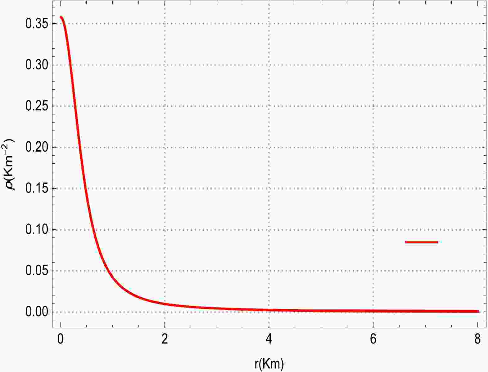
$({\rm e}^{2\psi(r)})'=({\rm e}^{2\lambda(r)})'=0$ when$ r=0 $ . In this analysis, we evalute the graphical impact of various polytropic models with numerous physical properties such as the matter density, pressure ($ P_{r} $ and$ P_{t} $ ), pressure anisotropy, mass function, electric field, speed of sound, compactness, electric charge, and adiabatic index. We observe the physical viability of matter density for the evolution of the compact sphere model displayed in Fig. 1. It can be observed from Fig. 1 that the behavior of the matter density is non-negative, as well as non-singular, throughout the interior region of the star. It is also evident that the matter density is maximum near the center of the star compared to that on the surface of the star. This characteristic suggests that the presented model predicts an ultra compact relativistic object. In Fig. 2, we depict the evolutionary nature of the radial and tangential pressures for the modeling of stellar interior compact stars. One can easily infer from Fig. 2 that the radial and tangential pressures depict a positive evolution behavior as they remain regular (finite) and non-singular at each point inside the compact stellar body. It is also evident here that both material quantities increase from the center and decrease gradually toward the boundary surface.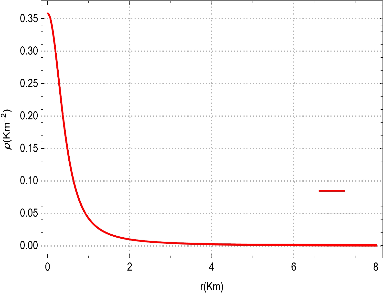
Figure 1. (color online) Evolutionary behavior of the matter density as a function of the radial coordinate r for
$ \xi=3 $ and$ \alpha=1.15 $ .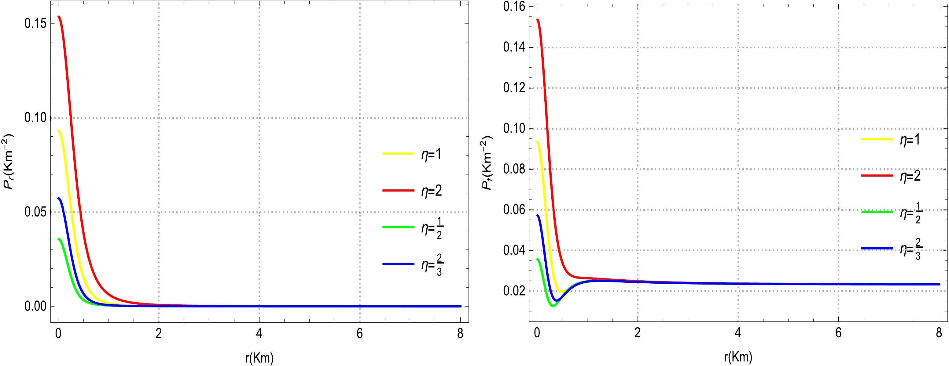
Figure 2. (color online) Physical evolution of radial and tangential pressures vs r for different choices of
$\eta=1,~ 2,~ \dfrac{1}{2},~ \dfrac{2}{3},~ \xi=3$ ,$\mathcal{A}=0.01,~ \mathcal{B}=0.7$ , and$ \alpha=1.15 $ .In terms of static and spherically symmetric anisotropic COs, we describe some viable consequences of Einstein's equations of motion with their standard physical features. These consequences can be determined in the absence of pressure, an isotropic source, and an anisotropic fluid. Nevertheless, several rigorous studies argue that excessive compact relativistic stars are not formed from isotropic sources. In certain bounds, structures with unpredictable physical implications are formed for the illustration of pressure anisotropy. In particular, we briefly review the anisotropic matter field based on the energy-momentum tensor that characterizes the physical composition of a stellar CO interior. Indeed, an anisotropic matter field is an exceptional exotic choice for the modeling of stellar COs such as white dwarfs, quark made stars, neutron stars, and pulsars Jeans [118] was the first theorist to review the effects of anisotropic pressure on a self-gravitating relativistic dense star model. Moreover, studies have revealed that a pressure anisotropy may appear within the interior configuration of compact stars owing to various factors such as the superluminal fluid [19, 20, 113], phase period [118], and electromagnetic field [119]. Based on these vital facts, we examine the profile of pressure anisotropy for our proposed polytropic models based on Fig. 3. It can be easily observed from Fig. 3 that the evolution of the pressure anisotropy is positive, as well as regular (finite), within the star; however, at some limiting points, it deviates slightly from the standard position, possibly owing to the exotic nature of the fluid. This pressure anisotropy sharply increases from the center toward the boundary surface of the sphere, where
$ r=1 $ . In addition, this trend indicates that the pressure anisotropy demonstrates a repulsive nature, i.e.,$ P_{r}<P_{t} $ . This characteristic indicates that the interior core of the star has a high density owing to the increase in pressure anisotropy. Consequently, we can demonstrate that our proposed models of spherically dense compact stars are physically admissible, as well as potentially stable. Based on Fig. 4, we analyze the physical evolution of the effective mass function, as well as the electromagnetic field, for our compact star model. The behavior of the effective mass within the entire region of the star is non-negative as it is continuous (regular) at every point. Moreover, the effective mass rapidly increases from the center toward the boundary of the sphere and reaches a maximum value at$r\sim8$ . Based on these features, we can predict that our proposed star model is capable of developing an ultra dense relativistic star, as predicted in Ref. [88]. Moreover, one can notice from the right plot of Fig. 4 that the electromagnetic field is positive at every point inside the sphere as it is continuous (regular) everywhere, and it exhibits maximum evolutionary behavior near the core of the star and steadily decreases toward the boundary surface as the radial coordinate r increases.
Figure 3. (color online) Variational nature of pressure anisotropy versus r for various values of
$\eta=1,~ 2,~ \dfrac{1}{2},~ \dfrac{2}{3}, ~\xi=3$ ,$\mathcal{A}=0.01,~ \mathcal{B}=0.7$ , and$ \alpha=1.15 $ .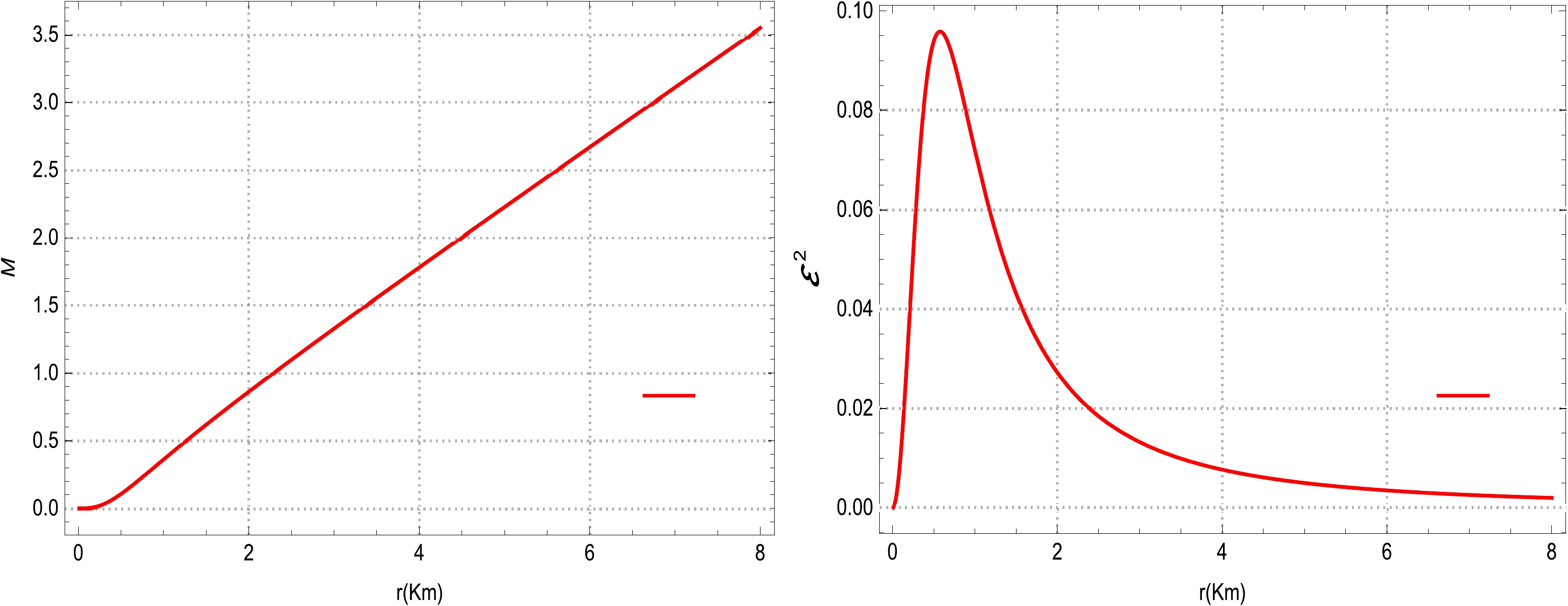
Figure 4. (color online) Physical variation in the effective mass function (left plot) and electromagnetic field (right plot) w.r.t. the radial distance r.
We investigate the evolutionary nature of the speed of sound
$\bigg(\dfrac{{\rm d}P_{r}}{{\rm d}\rho}$ and$\dfrac{{\rm d}P_{t}}{{\rm d}\rho}\bigg)$ for our polytropic models of compact stars for various choices of η (Fig. 5). It is evident from Fig. 5 that the trends followed by all curves for the speed of sound (left plot) with respect to their polytropic models suggest a positive nature at any interior point of the star. Moreover, the speed of sound (left plot) for our proposed polytropic models remains within a certain limit and does notcross the adequate bound, i.e.,$0 < \dfrac{{\rm d}P_{r}}{{\rm d}\rho}\leq1$ . Additionally,the behavior of the tangential speed of sound remains positive throughout the entire configuration of the star for all polytropic models, and the value does not cross the sufficientbound, i.e.,$0 < \dfrac{{\rm d}P_{t}}{{\rm d}\rho}\leq1$ (see Fig. 5 (right plot)).Moreover, the nature of the tangential speed of sound is regular (finite) at every interior point, and the speed gradually decreases from the center toward the boundary surface of the star. These features of the speed of sound strongly indicate that our compact star models are stable, as well as compatible with the prior result of the causality condition presented in Ref. [6].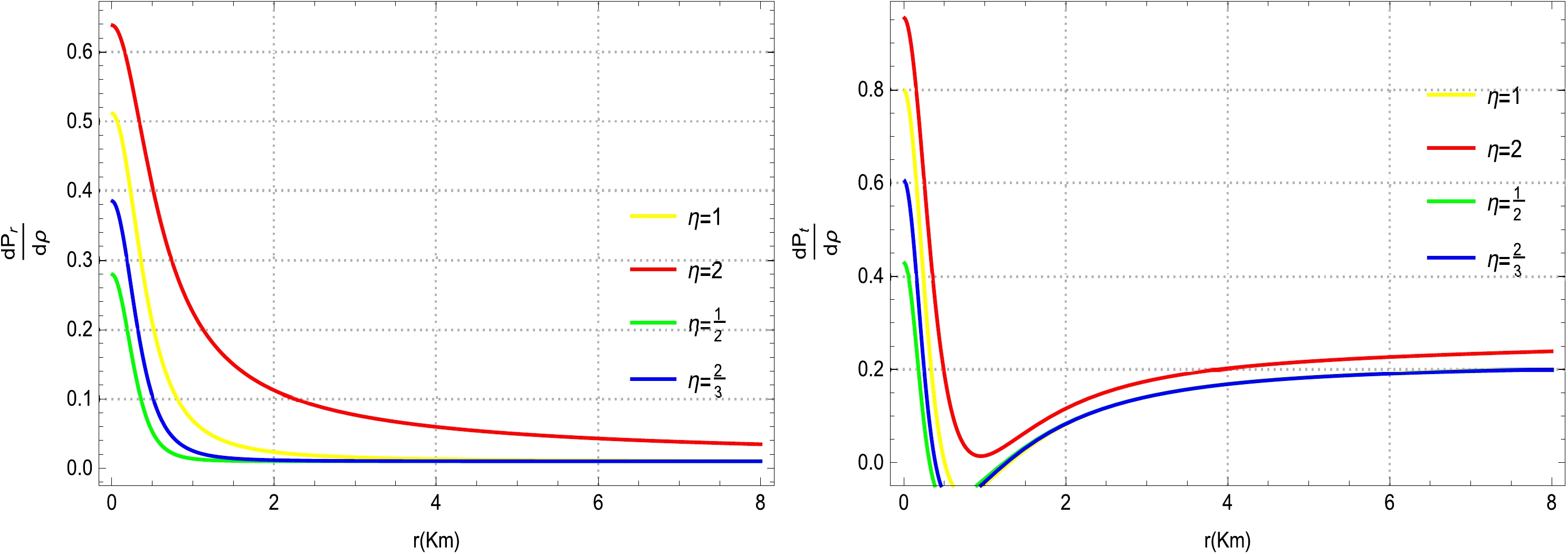
Figure 5. (color online) Physical variation in the sound speed
$\dfrac{{\rm d}P_{r}}{{\rm d}\rho}$ (left plot) and$\dfrac{{\rm d}P_{t}}{{\rm d}\rho}$ (right plot) versus r for certain values of$\eta=1,~ 2,~ \dfrac{1}{2},~ \dfrac{2}{3}$ ,$\xi=3,~ \mathcal{A}=0.01,~ \mathcal{B}=0.7$ , and$ \alpha=1.15 $ .Notably, a realistic relation between the compactness factor and electric charge is pivotal in confirming the non-violation of the stable configuration in the modeling of COs. For this assessment, Buchdahl pioneered the study on the compactness factor for a static and spherically symmetric perfect fluid sphere [120]. According to Buchdahl, the maximum allowable ratio of the mass-radius for a CO can be less than
$ \dfrac{4}{9} $ , i.e.,$ \left(\dfrac{2M}{r_{b}}<\dfrac{8}{9}\right) $ . Mak et al. [121] and Andr$ \acute{e} $ asson [122] generalized this condition for interior charged compact star models. The term$ \dfrac{M}{r_{b}} $ is considered as the compactness factor that categorizes astrophysical COs into the following: normal star:$ \dfrac{M}{r_{b}}\sim 10^{-5} $ , white dwarf:$ \dfrac{M}{r_{b}}\sim 10^{-3} $ , neutron star:$ 0.1<\dfrac{M}{r_{b}}< 0.25 $ , ultra dense CO:$ 0.25<\dfrac{M}{r_{b}}<0.50 $ , and black hole:$ \dfrac{M}{r_{b}}=0.50 $ [123]. The numerically estimated values for the electric charge and compactness factor for our compact star model are listed in Table 1. It can be observed that the numerically estimated ratio of the charge to radius for a given compactness lies in the allowable limit and does not violate the Buchdahl condition for a charged CO. In addition to this allowable limit, there exists another upper limit that should necessarily be satisfied as the maximum allowed compactness and charge-radius ratio, i.e.,$ \left(\dfrac{Q^{2}}{r^{2}_{b}}<\dfrac{2M}{r_{b}}<\dfrac{8}{9}\right )$ . This discussion confirms that our compact star model satisfiesthe necessary Buchdahl condition for a charged CO and may be able to predict an ultra dense CO. We present another interesting comparison with previous studies regarding the computed amount of the total electric charge in Coulomb units in Table 1. We observe that the total charge on the surface has a Coulomb unit of 3.7880$ \times 10^{20} $ [C] for the proposed star with an arbitrary mass and radius of${M}$ =3.54976 [km] and$ r_{b}=8 $ [km], respectively. An investigation on the$ f(R,T) $ gravity in the background of two geometrical techniques was conducted by Maurya et al. [100]; here, the authors estimated the maximum amount of electric charge as 2.46693$ \times 10^{20} $ [C] and 2.58885$ \times 10^{20} $ [C] for two different charged compact star models. Within the realm of the$ GR $ , the same research team [98, 104] reported the maximum amount of electric charge in Coulomb units for anisotropic strange star candidates as 4.04378$ \times 10^{19} $ [C] for a radius of 8 [km] and as 1.638631$ \times 10^{20} $ [C] for a radius of 7.1 [km]. They also estimated corresponding values of 7.5317$ \times 10^{19} $ [C] for PSR J1664-2230 and$ 9.8951 \times 10^{19} $ [C] for PSR 1937+21. Based on this detailed analysis, we can conclude that our computed amount of electric charge on the surface in Coulomb units is better compared with previous values.$r_{b} \; /{\rm km}$ 

$ {\boldsymbol{M}}({\boldsymbol{M}}_\odot) $ 

${\boldsymbol{M} }\,/{\rm km}$ 

Q Coulomb C $ \dfrac{Q}{r_{b}} $ 

$ \dfrac{Q^{2}}{r^{2}_{b}} $ 

$ \dfrac{{{M}}}{r_{b}}<\dfrac{4}{9} $ 

$ \dfrac{2{{M}}}{r_{b}} <\dfrac{8}{9}$ 

8 2.40661 3.54976 3.7880×10²⁰ 0.406133 0.164944 0.443720 0.887441 Table 1. Numerically estimated values of the total electric charge and compactness parameter corresponding to the arbitrary radius and mass of the compact star.
Moreover, the physical behavior of the compactness factor and electric charge for our compact star model is depicted in Fig. 6. It can be clearly observed that the trends followed by the compactness (left plot) factor and electric charge (right plot) suggest positive evolutions at every point in the stellar interior, as these factors are non-singular within the entire region of the star. The compactness parameter and electric charge increase with the radial coordinate r and attain maximum values at the boundary sphere. Additionally, the Buchdahl limit for a charged CO is obeyed, and the necessary condition is not violated. Moreover, the mass-radius relation is
$ 0.25<\dfrac{M}{r_{b}}<0.50 $ , which corresponds to a stable neutron star and ultra dense compact star.
Figure 6. (color online) Physical variation in the compactness (left plot) and total electric charge (right plot) versus the radial distance r.
Another important condition to ensure the stability equilibrium of the model is the adiabatic index. The adiabatic index denotes a ratio between two specific heats [124]. In testing the consistency of the model, the relativistic adiabatic index Γ along the radial direction plays a prime role. Here, the radial direction is vital because under the influence of anisotropy, the system is reformed from a spherically symmetric one along the radial direction to prevent gravitational collapse. In previous studies [125, 126], detailed analyses were performed using different mathematical mechanisms to compute the relativistic adiabatic index, along with its critical value, to ensure the stability of the stellar compact models. The relativistic adiabatic index can be expressed as
$ \Gamma=\frac{\rho+P_{r}}{P_{r}}\frac{{\rm d}P_{r}}{{\rm d}\rho}. $

(59) One can affirm that for system stability, the relativistic adiabatic index becomes
$\Gamma\geq\Gamma_{\rm crit}$ . The critical value of the relativistic adiabatic index can be evaluated by the following expression$ \Gamma_{\rm crit}=\frac{4}{3}+\frac{19u}{21}. $

(60) In Fig. 7, we plot the physical behavior of the relativistic adiabatic index Γ for different polytropic models. It can be observed from Fig. 7 that all curves of the adiabatic relativistic index corresponding to various polytropic models suggest positive evolutions within the stellar object, along with a gradual decrease from the center toward the boundary of the sphere. In addition, these polytropic models confirm the stability of our stellar CO by satisfying the relativistic condition
$ \Gamma>\dfrac{4}{3} $ (see Fig. 7). Consequently, we can firmly assert that the suggested models are potentially well behaved and able to model a CO. Moreover, we compute the numerical values of Γ, along with its critical value, and the results are summarized in Table 2. Based on these computed numerical values, one can infer that the condition in Eq. (60) ensures the stability equilibrium of our models.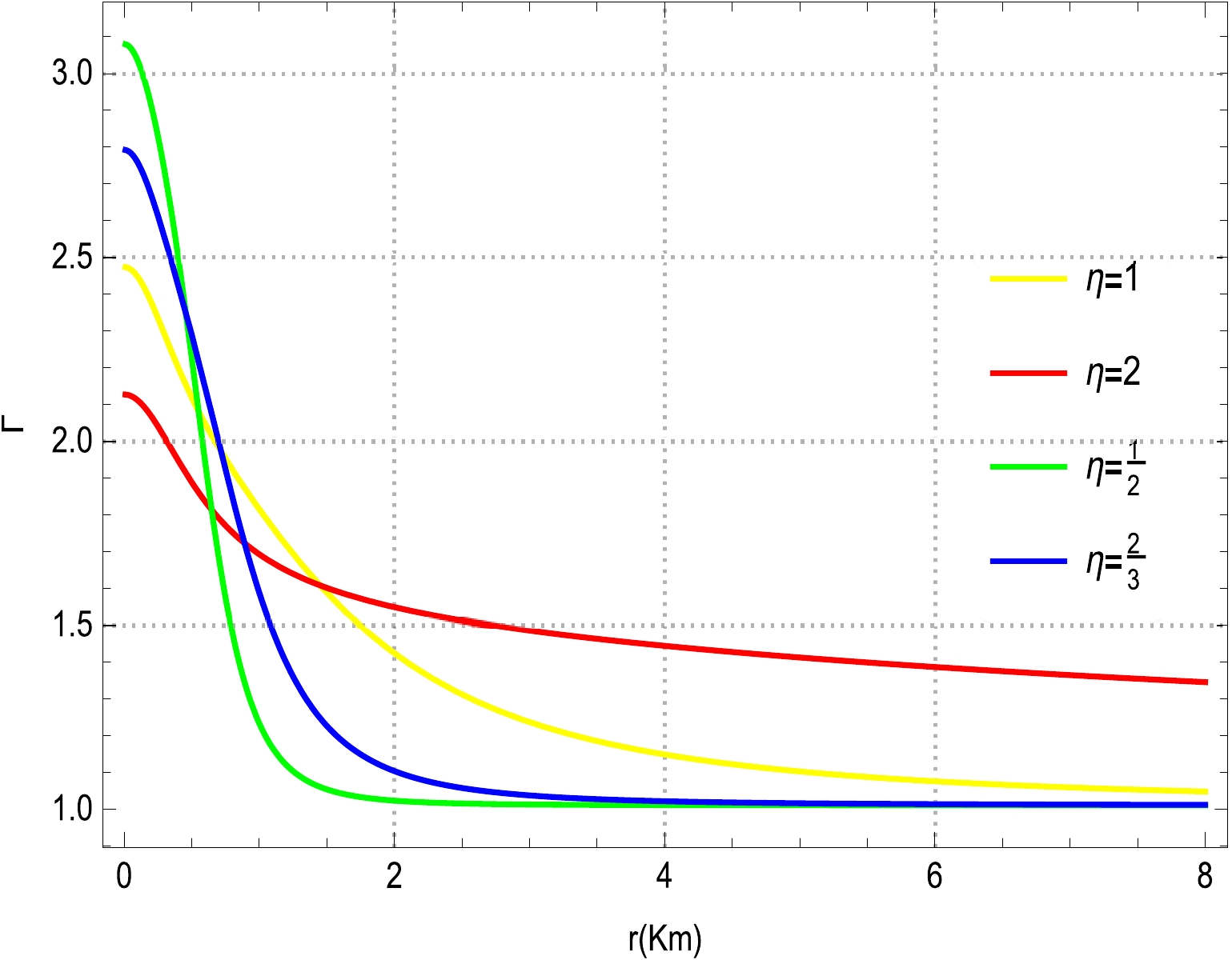
Figure 7. (color online) Physical behavior of the adiabatic index Γ vs the radial distance r.
$ \Gamma(0) $ 

$ \Gamma(0) $ 

$ \Gamma(0) $ 

$ \Gamma(0) $ 

Γ(crit) $( {Model-1})$ 

$( {Model-2})$ 

$( {Model-3})$ 

$( {Model-4})$ 

2.47297 2.12667 3.07882 2.79126 1.73479 Table 2. Numerical values of the adiabatic index
$ \Gamma(0) $ and its critical values Γ(crit) for the proposed polytropic models -
Modeling a stellar relativistic CO may be possible using underdeveloped polytropic models with the generalized polytropic EoS in the Finch-Skea geometry. The authors of Ref. [127] revealed that a non-linear EoS can reproduce the features of dark matter and dark energy, collectively aiding the explanation of the inflationary phases of the universe. In this study, we generated new exact analytical solutions for static and spherically symmetric objects containing anisotropic matter. The obtained solutions to the generalized polytropic EoS were constructed to model charged anisotropic compact stars corresponding to the Finch-Skea spacetime. We graphically examined that the models were physically admissible, as well as potentially sustainable. We determined that the gravitational potential and matter quantities were non-singular, as they were very consistent inside the celestial sphere. For
$ \eta=1 $ , we could simply adapt our solution to this particular case, as recommended by Feroze and Siddique [59]. These solutions may be helpful in the modeling of relativistic COs considering particular matter distributions owing to the generalized polytropic EoS. In future studies, it may be interesting to differentiate the resulting solutions to obtain charged and uncharged astrophysical COs, such as$ SAX J 1808.4 $ -3658, as studied by Mafa Takisa and Maharaj [57] and Dey et al. [128]. Furthermore, the construction of a charged relativistic astrophysical compact sphere, which is highly dense, would require a very fine-tuned model. Additionally, we can convert our results into new uncharged anisotropic solutions by excluding the electric charge. This study reveals that the Finch-Skea spacetime is physically suitable for the formation of astronomical COs. From this understanding, we derive the following conclusions based on our proposed solutions:● Our results for the matter variables (ρ,
$ P_{r} $ , and$ P_{t} $ ) confirmed that they are regular and well behaved throughout the configuration of the stellar object, as shown in Figs. 1 and 2. The non-negative and monotonically decreasing nature of such variables could be evidently observed in the graphical plots. Furthermore, we noticed that near the central core of the star, these variables gradually increased and sharply vanished at the boundary of the star, where r is the highest. These implications ultimately suggest that our models can adequately model ultra dense relativistic compact stars.● From Fig. 3, we could clearly observe that the anisotropy in pressure was evolutionary in nature and continuous at every point inside the stellar body. Additionally, it was observed that the pressure anisotropy had a repulsive trend, i.e.,
$ P_{r}<P_{t} $ . This behavior indicates that our models are well-consistent and can predict ultra dense COs.● The graphical behavior depicted in Fig. 4 reveals that the mass function (left plot) rapidly increases from the center toward the boundary of the star, further indicating that the present model is viable and potentially stable. Moreover, we plotted the physical evolution of the electromagnetic field for our compact star model in Fig. 4 (right plot). The electromagnetic field presented non-negative evolution at every point inside the sphere as it was uniform throughout the sphere. It appeared to be a monotonically decreasing function of the radial coordinate r and disappeared at the boundary of the star.
● We investigated the physical impact of the causality condition
$\bigg(\dfrac{{\rm d} {P_{r}}}{{\rm d}\rho}$ and$\dfrac{{\rm d} {P_{t}}}{{\rm d}\rho} \bigg)$ on our compact star, as shown in Fig. 5. The evolution of each curve for the causality condition$\left(\dfrac{{\rm d} {P_{r}}}{{\rm d}\rho} \right)$ remained in the appropriate range and satisfied$0 < \dfrac{{\rm d} {P_{r}}}{{\rm d}\rho}\leq1$ . Moreover, the transverse sound speed was uniform at each point inside the star, as well as non-negative throughout the entire region. All trends followed by the transverse speed of sound with respect to the various choices of η demonstrated good agreement and did not breach the sufficient limit of$0 < \dfrac{{\rm d} {P_{t}}}{{\rm d}\rho}\leq1$ .The causality condition proved that the presented models of the compact star are stable.● The variations in the compactness factor and electric charge are plotted against r in Fig. 6. It is evident from Fig. 6 that the nature of both these plots (left and right) is continuous at all points in the interior of the star. The figure also indicates that the compactness and electric charge are monotonically increasing functions of r, and these factors attain their maximum values at
$r\sim8$ . In addition, the Buchdahl condition for a charged CO remains within the allowable limit and satisfies the necessary boundary.● We present the physical behavior of the adiabatic relativistic index Γ for the proposed polytropic models inFig. 7. All curves of Γ corresponding to various choices of η are stable at every point within the compact sphere.Table 2 also indicates that the values of the adiabatic relativistic index for all models remain greater than the critical value of the adiabatic index throughout the celestial system, representing a stable equilibrium position for the creation of a viable CO.
In conclusion, the features obtained from the generalized polytropic EoS, along with the Finch-Skea ansatz, are quite favorable and potentially stable in hydrostatic equilibrium for describing the gravitational aspects of astrophysical COs. Several physical conditions are satisfied considering different criterions such as the mass function, electric field, causality bounds, the Buchdahl condition with a charge to radius ratio, the adiabatic index, and its critical value. Particularly, our estimated value for the compactness was close to the Buchdahl limit and was at the upper bound of the charge-radius ratio for a charged CO (see Table 1). Another intriguing aspect to note is that our computed amount of the total electric charge at the boundary in Coulomb units was 3.7880
$ \times 10^{20} $ [C] with an arbitrary mass of M=3.54976 [km] and radius of$ r_{b}=8 $ [km], which is better than the previous result reported in Refs. [98, 100, 104]. We ensured the stability of our models by inspecting the relativistic adiabatic index, along with its critical value. Both the stability conditions were found to be in good agreement and satisfied the sufficient relativistic physical bounds (see Table 2). These attributes confirm the maximum gravitational stability constraints required to create a viable ultra dense compact star model and neutron star. The results obtained in the presence of an electric charge are novel and consider a more general framework owing to the generalized polytropic EoS compared to the results of previous studies [107]. -
The results of the pressure (
$ P_{r} $ and$ P_{t} $ ) and pressure anisotropy (Δ) for different choices of the polytropic index,$\eta=1,~ 2,~ \dfrac{2}{3},~ \dfrac{1}{2}$ , are given below● For
$ \eta=1 $ $ P_{r} = \frac{\mathcal{A}}{8\pi} \Bigg[\frac{3\xi+\xi^2 x-\alpha x}{(1+\xi x)^{2}}\Bigg]+\frac{\xi}{8\pi}\Bigg[\frac{3\xi+\xi^2 x-\alpha x}{(1+\xi x)^{2}}\Bigg]^{2}, \tag{A1} $

$ \begin{aligned}[b]\\ P_{t}=&\mathcal{A}\ \Bigg[\frac{3\xi+\xi^{2}x-\alpha x}{8\pi(1+\xi x)^{2}}\Bigg]+\xi\Bigg[\frac{3\xi +\xi^{2}x-\alpha x}{8\pi(1+\xi x)^{2}}\Bigg]^{2}+\frac{x}{2\pi(1+\xi x)} \Bigg[\frac{i(i-1)\xi^{2}}{(1+\xi x)^{2}}+\frac{2\ i\ \xi\ \dot{L}(x)}{1+\xi x}\\ &+\dot{L}(x)^{2}+\ddot{L}(x)\Bigg]-\frac{\xi x}{4\pi(1+\xi x)^{2}}\Bigg[\frac{i\ \xi}{1+\xi x}+\dot{L}(x)\Bigg]+ \frac{\xi^{2}x}{8\pi(1+\xi x)^{2}}-\frac{\alpha x}{4\pi(1+\xi x)}, \end{aligned} \tag{A2} $ 
$ \Delta=\frac{x}{2\pi(1+\xi x)}\Bigg[\frac{i(i-1)\xi^{2}}{(1+\xi x)^{2}}+\frac{2\ i\ \xi\ \dot{L}(x)}{1+\xi x}+\dot{L}(x)^{2}+\ddot{L}(x)\Bigg] -\frac{\xi x}{4\pi(1+\xi x)^{2}}\Bigg[\frac{i\ \xi}{1+\xi x}+\dot{L}(x)\Bigg]+ \frac{\xi^{2}x}{8\pi(1+\xi x)^{2}} -\frac{\alpha x}{4\pi(1+\xi x)}. \tag{A3} $

Here, the derivative w.r.t the variable x is represented with a ·, and the functions
$ \dot{L}(x) $ and$ \ddot{L}(x) $ are described as$ \begin{aligned}[b] \dot{L}(x)=&\frac{(\xi^{2}-\alpha)}{4a}\ (\mathcal{A}+1)+ \frac{\mathcal{B}\ (2\xi^{2}+ \alpha)}{32\pi\xi^{2}}\left[\frac{4\xi^{2}+2\xi^{3} x-2\xi x\alpha-\alpha}{(1+\xi x)^{3}}\right],\\ \ddot{L}(x)=&-\frac{\mathcal{B}\ (2\xi^{2}+\alpha)}{32 \pi \xi}\left[\frac{10\xi^{2}+4\xi^{3} x-4\xi x\alpha-\alpha}{(1+\xi x)^{4}}\right]. \end{aligned} $

● For
$ \eta=2 $ $ P_{r}=\mathcal{A} \Bigg[\frac{3\xi+\xi^2 x-\alpha x}{8\pi(1+\xi x)^{2}}\Bigg]+\mathcal{B} \Bigg[\frac{3\xi+\xi^2 x-\alpha x}{8\pi(1+\xi x)^{2}}\Bigg]^{\frac{3}{2}}, \tag{A4} $

$ \begin{aligned}[b] P_{t}=&\mathcal{A}\ \Bigg[\frac{3\xi+\xi^{2}x-\alpha x}{8\pi(1+\xi x)^{2}}\Bigg]+ \mathcal{B}\Bigg[\frac{3\xi+\xi^{2}x-\alpha x}{8\pi(1+\xi x)^{2}}\Bigg]^{\frac{3}{2}}+\frac{x}{2\pi(1+\xi x)}\Bigg[\frac{\rm d}{{\rm d}x}\Bigg[\frac{\xi j}{1+\xi x}+\frac{k \sqrt{\xi(2\xi^{2}+\alpha)}}{\sqrt{3\xi+(\xi^{2}-\alpha)x}\ (1+\xi x)}+\dot{M}(x)\Bigg]+\frac{\dot{y}^{2}}{y^{2}}\Bigg] \\ &-\frac{\xi x}{4\pi(1+\xi x)^{2}}\Bigg[\frac{\xi j}{1+\xi x}+\frac{k \sqrt{\xi(2\xi^{2}+\alpha)}}{\sqrt{3\xi+(\xi^{2}-\alpha)x}\ (1+\xi x)}+\dot{M}(x)\Bigg] +\frac{\xi^{2}x}{8\pi(1+\xi x)^{2}}-\frac{\alpha x}{4\pi(1+\xi x)}, \end{aligned}\tag{A5} $

$ \begin{aligned}[b] \Delta=&\frac{x}{2\pi(1+\xi x)}\Bigg[\frac{\rm d}{{\rm d}x}\Bigg[\frac{\xi j}{1+\xi x}+\frac{k \sqrt{\xi(2\xi^{2}+\alpha)}}{\sqrt{3\xi+(\xi^{2}-\alpha)x}\ (1+\xi x)}+\dot{M}(x)\Bigg]+\frac{\dot{y}^{2}}{y^{2}}\Bigg]-\frac{\xi x}{4\pi(1+\xi x)^{2}}\Bigg[\frac{\xi j}{1+\xi x}+\frac{k \sqrt{\xi(2\xi^{2}+\alpha)}}{\sqrt{3\xi+(\xi^{2}-\alpha)x}\ (1+\xi x)}\\ &+\dot{M}(x)\Bigg]+\frac{\xi^{2}x}{8\pi(1+\xi x)^{2}}-\frac{\alpha x}{4\pi(1+\xi x)}. \end{aligned} \tag{A6} $

The functions
$ \dot{M}(x) $ and$ \dfrac{\dot{y}}{y} $ are defined as$ \begin{aligned}[b] \frac{\dot{y}}{y}=&\frac{\xi j}{1+\xi x}+\frac{k \sqrt{\xi(2\xi^{2}+\alpha)}}{\sqrt{3\xi+(\xi^{2}-\alpha)x}\ (1+\xi x)}+\dot{M}(x),\\ \dot{M}(x)=&\frac{(\xi^{2}-\alpha)}{4\xi}(\mathcal{A}+1)+\frac{\mathcal{B}\ [(\xi^{2}-\alpha)x+3\xi]^{-\frac{1}{2}}}{16\ \xi^{2}\ \sqrt{2\pi}\ (1+\xi x)^{2}}\Big[\xi^{3}x(6\xi^{2}+2\xi^{3}x-9\alpha)+3\alpha^{2}(1+3\xi x) -4\xi^{4}(-3+x^{2}\alpha)+\xi^{2}\alpha(3+2x^{2}\alpha)\Big]. \end{aligned} $

● For
$ \eta=2/3 $ $ P_{r}=\mathcal{A}\ \Big[\frac{3\xi+\xi^2 x-\alpha x}{8\pi(1+\xi x)^{2}}\Big]+\mathcal{B}\ \Big[\frac{3\xi+\xi^2 x-\alpha x}{8\pi(1+\xi x)^{2}}\Big]^{\frac{5}{2}}, \tag{A7} $

$ \begin{aligned}[b] P_{t}=&\mathcal{A}\ \Bigg[\frac{3\xi+\xi^{2}x-\alpha x}{8\pi(1+\xi x)^{2}}\Bigg]+\mathcal{B}\ \Bigg[\frac{3\xi+ \xi^{2}x-\alpha x}{8\pi(1+\xi x)^{2}}\Bigg]^{\frac{5}{2}}+\frac{x}{2\pi(1+\xi x)}\Bigg[\frac{\rm d}{{\rm d}x}\Bigg(\frac{\xi l}{1+\xi x}+\frac{m \sqrt{\xi(2\xi^{2}+\alpha)}}{\sqrt{3\xi+(\xi^{2}-\alpha)x}\ (1+\xi x)}+\dot{N}(x)\Bigg)+\frac{\dot{y}^{2}}{y^{2}}\Bigg]\\ & -\frac{\xi x}{4\pi(1+\xi x)^{2}}\Bigg[\frac{\xi l}{1+\xi x}+\frac{m \sqrt{\xi(2\xi^{2}+\alpha)}}{\sqrt{3\xi+(\xi^{2}-\alpha)x}\ (1+\xi x)}+\dot{N}(x)\Bigg] +\frac{\xi^{2}x}{8\pi(1+\xi x)^{2}}-\frac{\alpha x}{4\pi(1+\xi x)}, \end{aligned} \tag{A8} $

$ \begin{aligned}[b] \Delta=&\frac{x}{2\pi(1+\xi x)}\Bigg[\frac{\rm d}{{\rm d}x}\Bigg(\frac{\xi l}{1+\xi x}+\frac{m \sqrt{\xi(2\xi^{2}+\alpha)}}{\sqrt{3\xi+(\xi^{2}-\alpha)x}\ (1+\xi x)}+\dot{N}(x)\Bigg)+\frac{\dot{y}^{2}}{y^{2}}\Bigg]-\frac{\xi x}{4\pi(1+\xi x)^{2}}\Bigg[\frac{\xi l}{1+\xi x}\\ &+\frac{m \sqrt{\xi(2\xi^{2}+\alpha)}}{\sqrt{3\xi+(\xi^{2}-\alpha)x}\ (1+\xi x)}+\dot{N}(x)\Bigg]+\frac{\xi^{2}x}{8\pi(1+\xi x)^{2}}-\frac{\alpha x}{4\pi(1+\xi x)}. \end{aligned} \tag{A9} $

The functions
$ \dot{N}(x) $ and$ \dfrac{\dot{y}}{y} $ are given as$ \frac{\dot{y}}{y}=\frac{\xi l}{1+\xi x}+\frac{m \sqrt{\xi(2\xi^{2}+\alpha)}}{\sqrt{3\xi+(\xi^{2}-\alpha)x}\ (1+\xi x)}+\dot{N}(x),\; $

$ \begin{aligned}[b] \dot{N}(x)=&-\frac{\mathcal{B}\ (\xi^{2}-\alpha)\ \sqrt{(3\xi+(\xi^{2}-\alpha)x)}}{1536 \sqrt{2}\ \xi^{2}\ \pi^{\frac{3}{2}}}\Bigg[\frac{66(\xi^{2}-\alpha)}{(1+\xi x)^{2}}+\frac{26\ (2\xi^{2}+\alpha)}{(1+\xi x)^{3}}\Bigg]\\&-\frac{\mathcal{B} (\xi^{2}-\alpha)}{3072 \sqrt{2}\ \xi^{3} \pi^{\frac{3}{2}}\sqrt{(3\xi +(\xi^{2}-\alpha)x)}} \Bigg[\frac{33(\xi^{2}-\alpha)^{2}}{(1+\xi x)}+\frac{26(\xi^{2}-\alpha)(2\xi^{2}+\alpha)}{(1+\xi x)^{2}} \\&+\frac{8(2\xi^{2}+\alpha)^{2}}{(1+\xi x)^{3}}\Bigg]+\frac{\mathcal{B}\ \sqrt{(3\xi+(\xi^{2}-\alpha)x)}}{512\ \sqrt{2}\ \xi^{2}\ \pi^{\frac{3}{2}}}\times \Bigg[\frac{33(\xi^{2}-\alpha)^{2}}{(1+\xi x)^{2}} +\frac{26(\xi^{2}-\alpha)}{(1+\xi x)^{3}}(2\xi^{2}+\alpha)\\&+\frac{8(2\xi^{2}+\alpha)^{2}}{(1+\xi x)^{4}}\Bigg]. \end{aligned} $

● For
$ \eta=1/2 $ $ P_{r}=\mathcal{A}\ \left[\frac{3\xi+\xi^2 x-\alpha x}{8\pi(1+\xi x)^{2}}\right]+\mathcal{B}\ \left[\frac{3\xi+\xi^2 x-\alpha x}{8\pi(1+\xi x)^{2}}\right]^{3}, \tag{A10} $

$ \begin{aligned}[b] P_{t}=&\mathcal{A}\ \left[\frac{3\xi+\xi^{2}x-\alpha x}{8\pi(1+\xi x)^{2}}\right]+\mathcal{B}\ \left[\frac{3\xi +\xi^{2}x-\alpha x}{8\pi(1+\xi x)^{2}}\right]^{3}+ \frac{x}{2\pi(1+\xi x)}\Bigg[\frac{n(n-1)\xi^{2}}{(1+\xi x)^{2}}+\frac{2\ n\ \xi\ \dot{O}(x)}{(1+\xi x)}+\dot{O}(x)^{2} +\ddot{O}(x)\Bigg]\\ &-\frac{\xi x}{4\pi(1+\xi x)^{2}}\left[\frac{n\ \xi}{(1+\xi x)}+\dot{O}(x)\right] +\frac{\xi^{2} x}{8\pi(1+\xi x)^{2}}-\frac{\alpha x}{4\pi(1+\xi x)}, \end{aligned} \tag{A11} $

$ \Delta=\frac{x}{2\pi(1+\xi x)}\left[\frac{n(n-1)\xi^{2}}{(1+\xi x)^{2}}+ \frac{n\ \xi\ \dot{O}(x)}{(1+\xi x)}+\dot{O}(x)^{2}+\ddot{O}(x)\right] -\frac{\xi x}{4\pi(1+\xi x)^{2}}\Bigg[\frac{n\ \xi}{2(1+\xi x)}+\dot{O}(x)\Bigg]+ \frac{\xi^{2}x}{8\pi(1+\xi x)^{2}} -\frac{\alpha x}{4\pi(1+\xi x)}. \tag{A12} $

The functions
$ \dot{O}(x) $ and$ \ddot{O}(x) $ are described as follows:$ \nonumber \dot{O}(x)=\frac{(\xi^{2}-\alpha)}{4\xi}\ (\mathcal{A}+1)+ \frac{\mathcal{B}}{256\pi^{2}}\left[\frac{(3\xi+\xi^{2} x-\alpha x)^{3}}{(1+\xi x)^{5}}\right], $

$ \nonumber \ddot{O}(x)=-\frac{\mathcal{B}}{256 \pi^{2}}\left[\frac{[2\xi^{2}(6+\xi x)+\alpha(3-2\xi x)](3\xi+\xi^{2} x-\alpha x)^{2}}{(1+\xi x)^{6}}\right]. $

Relativistic polytropic models of charged anisotropic compact objects
- Received Date: 2022-09-20
- Available Online: 2023-03-15
Abstract: In this paper, we introduce new viable solutions to the Einstein-Maxwell field equations by incorporating the features of anisotropic matter distributions within the realm of the general theory of relativity (


 DownLoad: