


 Abstract
 HTML
HTML Reference
 Related
 PDF
PDF


-
Although recent data from the Large Hadron Collider (LHC) have been leaning increasingly in favor of the standard model (SM), the possibility of additional dynamics beyond the SM still remains. Several issues stemming from both theory and experiments cannot be resolved within the SM alone, thereby calling for new physics (NP). One such issue is the observed pattern of fermion masses and mixings. While several theoretical scenarios have been put forth to address this issue, a particularly interesting class is based on three Higgs doublets [1–5]. The idea involves connecting three fermionic generations to the three present scalar doublets by means of certain discrete symmetries so as to explain the observed fermion masses and mixings. Discrete symmetries such as
$ A_4, S_3, \Delta_{27}, Z_3 $ [6] are examples from a longer list that have been embedded in a three Higgs doublet model (3HDM) to produce the aforementioned effect.It is not possible to predict the exact number of scalar doublets present in nature from fundamental principles given that the electroweak (EW) ρ-parameter does not deviate from unity in the presence of doublets alone. In a
$C P$ -conserving 3HDM, one amongst the three$C P$ -even scalars must have a mass of approximately 125 GeV to comply with Higgs discovery. It is understood that the couplings of this scalar to fermions and gauge bosons will be scaled with respect to the corresponding SM values, and the scaling factors will contain mixing angles that connect the gauge basis to the mass eigenstates. However, as observed in a 2HDM, it is possible to obtain an "alignment-limit" in a 3HDM when the couplings coincide with the corresponding SM values. The signal strength data for the 125 GeV scalar are automatically satisfied in this limit. Of course, a 3HDM can be distinguished from a 2HDM at a collider owing to certain cascades of scalars that bear information on the intermediate scalars present. Given that there are no hints of such signals at the LHC, the current scenario allows for a 3HDM as much as it allows for a 2HDM.A 3HDM obeying global
$ S_3 $ -symmetry is one such example that permits the desired alignment through its scalar potential. However, an immediate fallout of an$ S_3 $ -symmetric Yukawa sector is the presence of flavor-changing neutral currents (FCNCs) at the tree-level. The parameters responsible must typically be small to satisfy the constraints from meson-mixing and meson-decays. A question then naturally arises on whether such smallness is due to a radiative effect. That is, whether the$ S_3 $ -symmetric Yukawa Lagrangian is part of larger symmetry at a high energy scale at which the FCNC parameters vanish, and following spontaneous breakdown of the larger symmetry, whether they assume appropriately small but non-zero values at the EW scale through evolution under the renormalization group (RG). We attempt to probe this possibility in this study.We compute one-loop RG equations (RGEs) for all Yukawa couplings pertaining to
$ S_3 $ -symmetry and identify those responsible for FCNCs. Without considering a specific UV-complete theory, we can assume that the FCNC couplings vanish at some scale Λ. Effective field theory below this scale then corresponds to the$ S_3 $ -symmetric 3HDM (S3 HDM). We reiterate that our goal is not to conduct an exhaustive survey of the parameter space of this model considering all possible flavor constraints, but to study the sensitivity of the FCNC parameters to the aforementioned RG evolution.The paper is organized as follows: Section II contains details of the
$ S_3 $ HDM. We present the analysis and results in Section III. Section IV comprises a discussion on the RG-running of the Yukawa couplings of the up- and down-sectors. Finally, we summarize and conclude in Section V. -
The
$ S_3 $ $ S_3 $ HDM is an extension of the SM based on the discrete group$ S_3 $ , which comprises three$Y = {1}/{2}$ scalar doublets$ \phi_1, \phi_2 $ , and$ \phi_3 $ . Of these,$ \phi_1 $ and$ \phi_2 $ rotate into each other as doublets under$ S_3 $ , whereas$ \phi_3 $ remains a singlet under the same conditions. Thus, the most general scalar potential consistent with the gauge as well as$ S_3 $ -symmetry is [7, 8]$ \begin{aligned}[b] V(\phi) =& \mu_{11}^2(\phi_1^\dagger\phi_1+\phi_2^\dagger\phi_2)+ \mu_{33}^2\phi_3^\dagger\phi_3+ \lambda_1 (\phi_1^\dagger\phi_1+\phi_2^\dagger\phi_2)^2\\& +\lambda_2 (\phi_1^\dagger\phi_2 -\phi_2^\dagger\phi_1)^2 +\lambda_3 \Big\{(\phi_1^\dagger\phi_2+\phi_2^\dagger\phi_1)^2 \\&+(\phi_1^\dagger\phi_1-\phi_2^\dagger\phi_2) ^2\Big\} +\lambda_4 \Big\{(\phi_3^\dagger\phi_1)(\phi_1^\dagger\phi_2+\phi_2^\dagger\phi_1)\\& +(\phi_3^\dagger\phi_2)(\phi_1^\dagger\phi_1-\phi_2^\dagger\phi_2) + {\rm h. c.}\Big\}\\ & +\lambda_5(\phi_3^\dagger\phi_3)(\phi_1^\dagger\phi_1+\phi_2^\dagger\phi_2) + \lambda_6 \Big\{(\phi_3^\dagger\phi_1)(\phi_1^\dagger\phi_3)\\&+(\phi_3^\dagger\phi_2)(\phi_2^\dagger\phi_3)\Big\} +\lambda_7 \Big\{(\phi_3^\dagger\phi_1)(\phi_3^\dagger\phi_1) \\&+ (\phi_3^\dagger\phi_2)(\phi_3^\dagger\phi_2) +{\rm h. c.}\Big\} +\lambda_8(\phi_3^\dagger\phi_3)^2 \,. \end{aligned}$

(1) We take all the quartic couplings to be real to forbid
$C P$ -violation arising from the scalar sector. Following EW symmetry breaking (EWSB), the doublets can be expressed as$ {\phi _i} = \frac{1}{{\sqrt 2 }}\left( {\begin{array}{*{20}{c}} {\sqrt 2 w_i^ + }\\ {{v_i} + {h_i} + i{z_i}} \end{array}} \right)\;{\rm{for}}\;i = 1,2,3.{\rm{ }} $

(2) The vacuum expectation values
$ v_1, v_2, v_3 $ satisfy$ v_1^2 + v_2^2 + v_3^2 = (246 \; \text{GeV})^2 $ . In terms of the mass eigenstates, the spectrum consists of three$C P$ -even scalars$ h, H_1, H_2 $ , two$C P$ -odd scalars$ A_1, A_2 $ , and two charged scalars$ H_1^+, H_2^+ $ . The scalars in the mass eigenbasis are connected to those in the gauge eigenbasis through unitary transformations, and the form of such unitary matrices depends on whether the$ S_3 $ -invariance of the scalar potential is exact or allowed to be broken by terms of mass dimension-2. In the case of exact$ S_3 $ symmetry, minimizing the scalar potential enforces$ v_1 = \sqrt{3} v_2 $ [7, 8] if the conditions obtained thereafter are to be consistent with$ S_3 $ -invariance. In this case, tan$\beta = {2 v_2}/{v_3}$ can be defined, similar to that in a 2HDM. Subsequently, the diagonalizing matrices can be parameterized by two mixing angles, i.e., α and the aforementioned β. Exact forms of the unitary matrices can be found in [7] and therefore are not shown here. Similar to the case of a 2HDM, the relation$\alpha = \beta - {\pi}/{2}$ corresponds to the alignment, when the couplings of h to fermions and gauge bosons become equal to their corresponding SM values. Therefore, apart from the radiatively induced$ h \rightarrow \gamma \gamma $ channel, the LHC data on the signal strengths of h corresponding to the other channels are automatically satisfied upon tending to the$\alpha = \beta - {\pi}/{2}$ limit.The perturbativity and unitarity bounds on the quartic couplings
$ \lambda_i $ place an upper bound of$ < 1 $ TeV on the non-standard masses of the model [9]. To increase the non-standard scalar masses (later we shall discuss why this is required to satisfy flavor physics constraints),$ S_3 $ -symmetry is softy broken by dimension-2 operators. Then, the$C P$ -even sector, for example, relates the mass eigenbasis to the gauge eigenbasis through the most general$ 3 \times 3 $ orthogonal matrix$ {\cal{O}} $ as follows:$\left( {\begin{array}{*{20}{c}} {{h_1}}\\ {{h_2}}\\ {{h_3}} \end{array}} \right) = \left( {\begin{array}{*{20}{c}} {{O_{11}}}&{{O_{12}}}&{{O_{13}}}\\ {{O_{21}}}&{{O_{22}}}&{{O_{23}}}\\ {{O_{31}}}&{{O_{32}}}&{{O_{33}}} \end{array}} \right)\left( {\begin{array}{*{20}{c}} h\\ {{H_1}}\\ {{H_2}} \end{array}} \right)$

(3) where
$ \begin{aligned}[b] O_{11} =& c_\phi c_\psi - c_\theta s_\phi s_\psi \,, \\ O_{12} = & -c_\phi s_\psi - c_\theta s_\phi c_\psi \,, \\ O_{13} =& s_\phi s_\theta \,, \\ O_{21} =& s_\phi c_\psi + c_\theta c_\phi s_\psi \,, \\ O_{22} =& -s_\phi s_\psi + c_\theta c_\phi c_\psi \,, \\ O_{23} = & -c_\phi s_\theta \,, \\ O_{31} = & s_\psi s_\theta \,, \\ O_{32} =& c_\psi s_\theta \,, \\ O_{33} = & c_\theta \,. \end{aligned}$

(4) $ \theta, \psi, \phi $ are the mixing angles.Now, the most general
$ S_3 $ -symmetric Yukawa potential for the up-type quark sector can be expressed as [7]$ \begin{aligned}[b] - {\cal{L}}_Y^{u} = & y_{1u} \Big( \overline Q_{1} \tilde\phi_3 u_{1R} + \overline Q_2 \tilde\phi_3 u_{2R} \Big) + y_{2u} \Big\{ \Big( \overline Q_{1}\tilde\phi_2 + \overline Q_2\tilde\phi_{1}\Big) u_{1R} \\&+ \Big( \overline Q_{1}\tilde\phi_{1} - \overline Q_2\tilde\phi_2 \Big)u_{2R} \Big\} + y_{3u} \overline Q_3\tilde\phi_3u_{3R} \\&+y_{4u} \overline Q_3 \Big( \tilde\phi_1 u_{1R} + \tilde\phi_2u_{2R} \Big) \\&+y_{5u} \Big( \overline Q_1 \tilde\phi_1 + \overline Q_2\tilde\phi_2 \Big) u_{3R} + {\rm{h.c.}} \end{aligned}$

(5) The Yukawa Lagrangian for the down-sector can be obtained by replacing
$ u \rightarrow d $ and$ \tilde{\phi} \rightarrow \phi $ . It should be noted that the fields$ u_i $ and$ d_i $ presented here do not denote physical quark fields. Their superpositions that are eigenstates will be given later. Following EWSB, the mass matrices of the fermions have the following texture [7]:$ \begin{aligned}[b]&{{\cal{M}}_f} = \frac{1}{{\sqrt 2 }}\left( {\begin{array}{*{20}{c}} {{y_{1f}}{v_3} + {y_{2f}}{v_2}}&{{y_{2f}}{v_1}}&{{y_{5f}}{v_1}}\\ {{y_{2f}}{v_1}}&{{y_{1f}}{v_3} - {y_{2f}}{v_2}}&{{y_{5f}}{v_2}}\\ {{y_{4f}}{v_1}}&{{y_{4f}}{v_2}}&{{y_{3f}}{v_3}} \end{array}} \right){\mkern 1mu} ,\\& {\rm{with}}\;f = u,d,l{\mkern 1mu} . \end{aligned} $

(6) Note that
$ {\cal{M}}_f $ in Eq. (6) is not Hermitian for$ y_{4f},y_{5f} \neq 0 $ and therefore is brought to a diagonal form by the following bi-unitary transformation:$ V_L^{\dagger} {\cal{M}}_f V_R = {\rm{diag}}(m_1,m_2,m_3), \tag{7a} $

$ m_1 = \frac{1}{\sqrt{2}}(y_{1f} v_3 - 2 y_{2f} v_2), \tag{7b} $

$ \begin{aligned}[b] m_{3,2} =& \frac{1}{2 \sqrt{2}}(2 y_{2f} v_2 + (y_{1f} + y_{3f}) v_3 \\ &\pm \sqrt{(y_{1f} v_3 + 2 y_{2f} v_2 - y_{3f} v_3)^2 + 16 y_{4f} y_{5f} v^2_2}) , \end{aligned}\tag{7c}$

where
$ m_i $ denotes the mass of the ith generation fermion. Therefore, it is possible to reproduce the observed values of the fermion masses by tuning the various Yukawa couplings and tan β appropriately.The matrices
$ V_L $ and$ V_R $ induce flavor-changing couplings with the Higgs in this model. The exact structure of the flavor-conserving and flavor-changing couplings can be found in Appendix B. -
From Appendix B, it can be seen that the flavor-changing couplings of SM Higgs involving the third generation of fermions are proportional to
$ y_{5f} $ , i.e., by taking$ y_{5f} $ to be negligible, one can ensure small flavor-changing couplings for the SM Higgs. Because the mass matrix of fermions is Hermitian for$ y_{4f}, y_{5f} = 0 $ ①, we assume$ y_{4f}, y_{5f} $ to be small for the entire analysis, which in turn gives small flavor-changing couplings to SM Higgs.Neglecting the small
$ y_{4f} $ and$ y_{5f} $ , the remaining three flavor-changing Yukawa couplings$ y_{1f} $ ,$ y_{2f} $ , and$ y_{3f} $ are fixed by the fermion masses$ m_1 $ ,$ m_2 $ , and$ m_3 $ as shown below.$ y_{1f} \simeq \frac{(m_1 + m_2)}{\sqrt{2} v_3} , \tag{9a}$

$ y_{2f} \simeq \frac{(m_2 - m_1)}{2 \sqrt{2} v_2} , \tag{9b} $

$ y_{3f} \simeq \frac{\sqrt{2} m_3}{v_3} . \tag{9c} $

For analysis, we vary
$ y_{4f} $ and$ y_{5f} $ as$ -0.005 \leq y_{4f} \leq 0.005 , \; -0.005 \leq y_{5f} \leq 0.005 . $

(10) $ v_1, v_2 $ , and$ v_3 $ can be expressed in terms of the mixing-angles β and γ as$ v_1 = v\; {\rm{sin}} \beta \; {\rm{cos}} \gamma , \tag{11a} $

$ v_2 = v\; {\rm{sin}} \beta \; {\rm{sin}} \gamma , \tag{11b} $

$ v_3 = v\; {\rm{cos}} \beta . \tag{11c} $

We set the masses of the mass eigenstates to be
$ m_h = 125.3\; {\rm{GeV}} , ~ m_{H_1} = m_{H_2} = m_{A_1} = m_{A_2} = 1 \; {\rm{TeV}}. $

To ensure that the lightest Higgs (h) of the model behaves as an SM Higgs, the couplings of h to gauge bosons and fermions (mentioned in Appendix B) are considered to be identical to those of the SM-Higgs via suitable choices of the angles
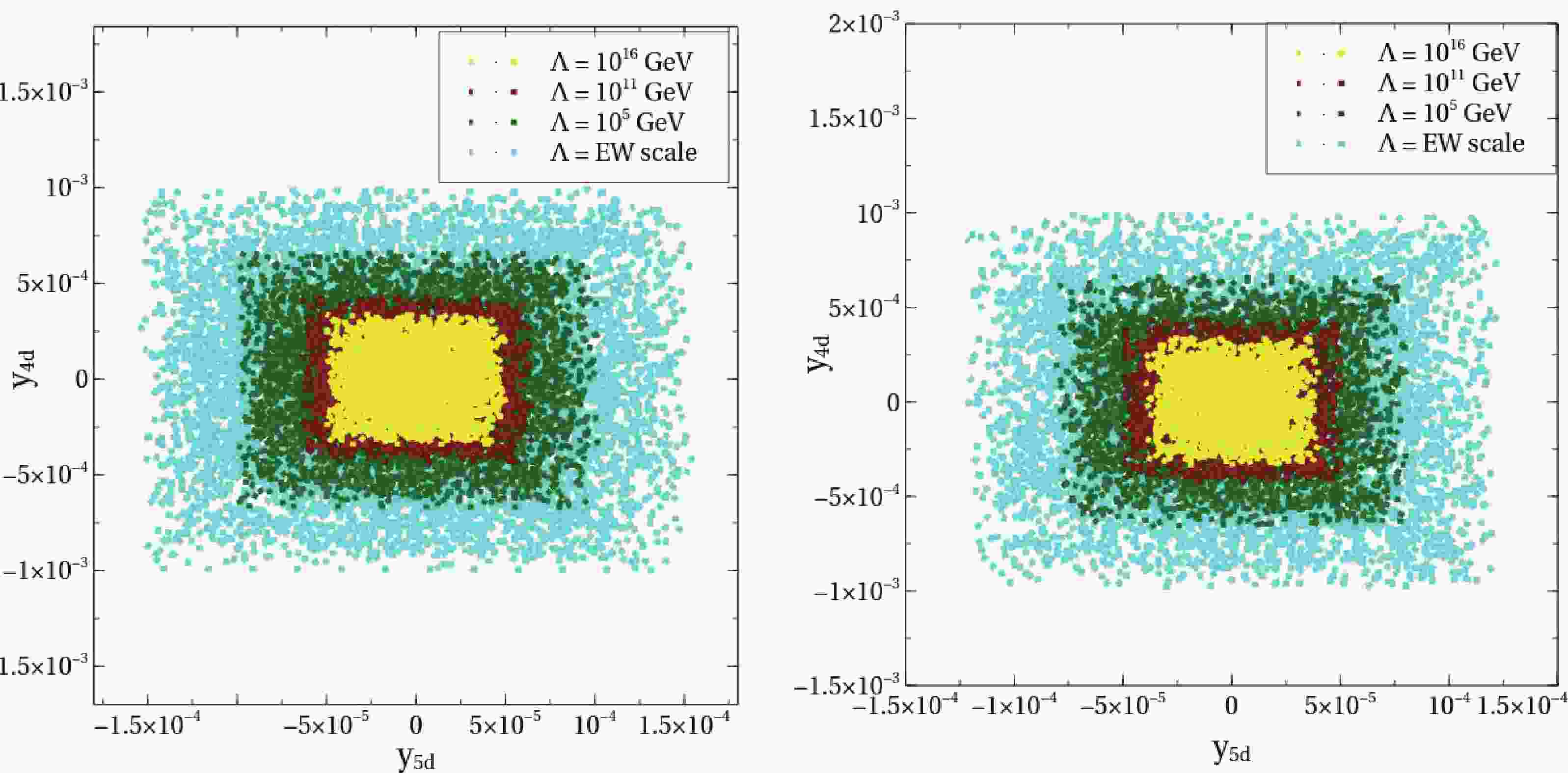
$ \beta, \gamma, \theta, \phi, \psi $ . While fixing γ, we take the flavor-changing couplings of h to the first two generations of the up and down type quarks, i.e.,$ y_{huc} $ and$ y_{hds} $ , to be zero. Thus, two benchmark points are chosen with different mixing angle values, as shown in Table 1. The values of$ y_{1f}, y_{2f}, y_{3f} $ at the EW scale are fixed by Eq. (9) and given in Table 1 for two different benchmark points BP1 and BP2. We take$ y_{4u} $ and$ y_{5u} $ to be zero at the EW scale. The corresponding values for$ y_{4d} $ and$ y_{5d} $ ($ << y_{1d}, y_{2d}, y_{3d} $ ) on the EW scale are fixed by flavor physics constraints, such as meson-mixing and meson-decays, as described in the next subsection. In Fig. 1, the cyan colored points represent the parameter space spanned by$ y_{4d} $ and$ y_{5d} $ at the EW scale for two different benchmark points.Benchmark Angle $ y_{iu} $ 

$ y_{id} $ 

BP1 $ \beta = $ 0.314159

$ y_{1u} = 0.00385 $ 

$ y_{1d} = 0.00030 $ 

$ \gamma = $ 0.839897

$ y_{2u} = 0.00794 $ 

$ y_{2d} = 0.00056 $ 

$ \theta = $ 1.20

$ y_{3u} = 0.99708 $ 

$ y_{3d} = 0.01872 $ 

$ \phi = $ 4.94

$ \psi = $ 1.82

BP2 $ \beta = $ 0.314159

$ y_{1u} = 0.00385 $ 

$ y_{1d} = 0.00030 $ 

$ \gamma = $ 1.12824

$ y_{2u} = 0.00654 $ 

$ y_{2d} = 0.00046 $ 

$ \theta = $ 2.10

$ y_{3u} = 0.99708 $ 

$ y_{3d} = 0.01872 $ 

$ \phi = $ 2.54

$ \psi = $ 1.49

Table 1. Angles and values of the Yukawa couplings
$ y_{iu} $ and$ y_{id} $ (for$ i = 1,2,3 $ ) at the electroweak scale for BP1 and BP2.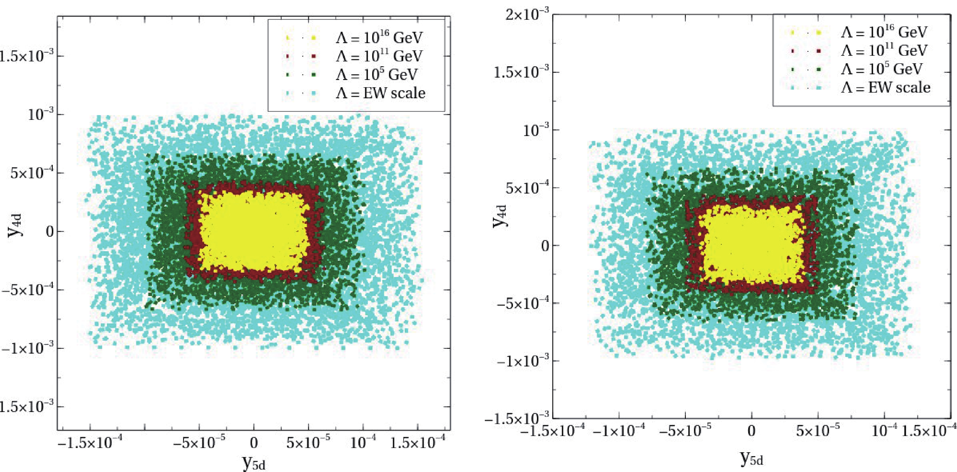
Figure 1. (color online) Parameter space spanned by
$ y_{4d} $ and$ y_{5d} $ for four different validity scales$ \Lambda = {\rm{EW-scale}}, 10^5, 10^{11}, 10^{16} $ GeV. The color coding is explained in the legends. -
In this subsection, we discuss the relevant processes contributing to the flavor physics constraints on the flavor-changing couplings to fermions.
-
The effective Hamiltonian for the process
$ B_s \rightarrow \mu^+ \mu^- $ can be calculated as [10]$\begin{aligned}[b] {\cal{H}}_{\rm{eff}} =& - \frac{G_{\rm F}}{\sqrt{2}} \frac{\alpha_{\rm{em}}}{\pi s_{\rm W}^2} V_{tb} V_{ts}^*(C_A {\cal{O}}_A + C_S {\cal{O}}_S\\& + C_P {\cal{O}}_P + C_S' {\cal{O}}_S' + C_P' {\cal{O}}_P') + {\rm{h.c.}} \, \end{aligned} $

(13) where
$G_{\rm F}$ is the Fermi constant,$ \alpha_{\rm{em}} $ is the fine structure constant,$ V_{ij} $ are the Cabibbo-Kobayashi-Masakawa (CKM) matrix elements, and$s_{\rm W} = {\rm {sin}} \theta_{\rm W}, \theta_{\rm W}$ being the Weinberg angle.The operators
$ {\cal{O}}_i $ and$ {\cal{O}}_i' $ are defined as$ {\cal{O}}_A = (\overline{s}\gamma_\mu P_L b)(\overline{\mu} \gamma^\mu \gamma_5 \mu)\,, $

(14) $ {\cal{O}}_S = (\overline{s} P_R b)(\overline{\mu} \mu) \,, $

(15) $ {\cal{O}}_P = (\overline{s} P_R b)(\overline{\mu} \gamma_5 \mu) \,, $

(16) $ {\cal{O}}_S' = (\overline{s} P_L b)(\overline{\mu} \mu) \,, $

(17) $ {\cal{O}}_P' = (\overline{s} P_L b)(\overline{\mu} \gamma_5 \mu) \,. $

(18) Here, the Wilson coefficient
$ C_A $ receives contributions from the SM only. In contrast, within the scope of the SM, the Wilson coefficients$ C_S^{\rm{SM}}, C_S^{'\rm{SM}}, C_P^{\rm{SM}}, C_P^{'\rm{SM}} $ from Higgs-penguin diagrams are highly suppressed.Therefore, we approximate
$ C_S^{\rm{SM}} = C_S^{'\rm{SM}} = C_P^{\rm{SM}} = C_P^{'\rm{SM}} = 0\,. $

(19) The NP contributions to the scalar and pseudoscalar Wilson coefficients are
$ C_S^{\rm{NP}} = - \kappa \sum\limits_{\Phi_S}\left(\frac{y_{\Phi_S sb}\; y_{\Phi_S \mu\mu}}{m_{\Phi_S}^2}\right),\; \Phi_S = h, H_1, H_2\,. $

(20) $ C_S^{'\rm{NP}} = C_S^{\rm{NP}} \,, $

(21) $ C_P^{\rm{NP}} = \kappa \sum\limits_{\Phi_P}\left(\frac{y_{\Phi_P sb}\; y_{\Phi_P \mu\mu}}{m_{\Phi_P}^2}\right),\; \Phi_P = A_1, A_2\,. $

(22) $ C_P^{'\rm{NP}} = - C_P^{\rm{NP}} \,, $

(23) where
$\kappa = \dfrac{\pi^2}{G_{\rm F}^2 m_W^2 V_{tb} V_{ts}^*}$ ,$ m_W $ is the mass of the W-boson,$ y_{\Phi_{S(P)} sb} $ is the Yukawa coupling between the scalar (pseudoscalar) and the first two generations of down quarks, and$ y_{\Phi_{S(P)} \mu \mu} $ is the Yukawa coupling between the scalar (pseudoscalar) and muons.From the Hamiltonian in Eq. (13), the branching ratio of the process
$ B_s \rightarrow \mu^+ \mu^- $ is [11, 12]$\begin{aligned}[b] {\rm{Br}}(B_s \rightarrow \mu^+ \mu^- ) =& \frac{\tau_{B_s} G_F^4 m_W^4}{8 \pi^5} |V_{tb} V_{ts}^*|^2 f_{B_s}^2 m_{B_s} m_\mu^2\\&\times \sqrt{ 1 - \frac{4 m_\mu^2}{m_{B_s}^2}} (|P|^2 + |S|^2)\,. \end{aligned} $

(24) where
$ m_{B_s} $ ,$ \tau_{B_s} $ , and$ f_{B_s} $ are the mass, lifetime, and decay constant of the$ B_s $ meson, respectively (values can be found in Ref. [13]), and$ \begin{aligned}[b] P \equiv & C_A + \frac{m_{B_s}^2}{2 m_\mu} \left(\frac{m_b}{m_b + m_s}\right) (C_P - C_P')\,, \\ S \equiv & \sqrt{ 1 - \frac{4 m_\mu^2}{m_{B_s}^2}} \frac{m_{B_s}^2}{2 m_\mu} \left(\frac{m_b}{m_b + m_s}\right) (C_S - C_S')\,, \end{aligned}$

(25) where
$ C_A = - \eta_Y Y_0 $ ,$ \eta_Y = 1.0113 $ ,$ Y_0 = \dfrac{x}{8} \Bigg(\dfrac{(4-x)}{(1-x)} + \dfrac{3 x \; {\rm{ln}}x}{(1-x)^2}\Bigg) $ ,$ x = \dfrac{m_t^2}{m_W^2} $ [14], and$ m_t $ ,$ m_b $ ,$ m_s $ , and$ m_\mu $ are the top quark, bottom quark, strange quark, and muon masses, respectively.For
$ B_s-\overline{B}_s $ oscillations, the measured branching ratio of$ B_s \rightarrow \mu^+ \mu^- $ should be calculated as a time-integrated value [15],$ \overline{{\cal{B}}}(B_s \rightarrow \mu^+ \mu^-) = \left(\frac{1 + {\cal{A}}_{\Delta \Gamma} y_s}{1 - y_s^2}\right) {\rm{Br}}(B_s \rightarrow \mu^+ \mu^-) \,. $

(26) where
$ \begin{aligned}[b] y_s =& \frac{\Gamma_s^L - \Gamma_s^H}{\Gamma_s^L + \Gamma_s^H} = \frac{\Delta \Gamma_s}{2 \Gamma_s} \,, \\ {\cal{A}}_{\Delta \Gamma} = & \frac{|P|^2 {{\rm{cos}}} (2 \phi_P - \phi_s^{NP}) - |S|^2 {{\rm{cos}}} (2 \phi_S - \phi_s^{NP}) }{|P|^2 + |S|^2} \,. \end{aligned}$

(27) Here,
$ \phi_{S(P)} $ are the phases associated with$ S(P) $ , and$ \phi_s^{\rm NP} $ is the CP phase originating from$ B_s-\overline{B}_s $ mixing. Within the scope of the SM,$ {\cal{A}}_{\Delta \Gamma} = 1 $ .$ \Gamma_s^L $ and$ \Gamma_s^H $ are the decay widths of the light and heavy mass eigenstates of$ B_s $ .Because the couplings
$ y_{\Phi_{S(P)} sb} $ and$ y_{\Phi_{S(P)} \mu \mu} $ are constrained by$ \overline{{\cal{B}}}(B_s \rightarrow \mu^+ \mu^-) $ data (Appendix B), it is clear that stringent bounds are imposed on the mixing angles and some Yukawa couplings in the down-sector.During the analysis, we use a
$ 2\sigma $ -experimental value of$ \overline{{\cal{B}}}(B_s \rightarrow \mu^+ \mu^-) $ (available in Table 2) for data fitting.Observables SM value Experimental value $ {\cal{\overline{B}}}(B_s \rightarrow \mu^+ \mu^-) $ (10

$ ^{-9}) $ 

3.66 $ \pm 0.14 $ [25]

3.09 $ ^{+0.46\; +0.15}_{-0.43\; -0.11} $ [25]

${\rm Br}(B_d \rightarrow \mu^+ \mu^-)$ (10

$ ^{-10}) $ 

1.03 $ \pm 0.05 $ [25]

1.2 $ ^{+0.8}_{-0.7}\pm 0.1 $ [25]

$ \Delta m_s $ (ps

$ ^{-1} $ )

18.3 $ \pm2.7 $ [26, 27]

17.749 $ \pm 0.019\; ({\rm{stat}})\pm 0.007\; ({\rm{syst.}}) $ [28–33]

$ \Delta m_d $ (ps

$ ^{-1} $ )

0.528 $ \pm 0.078 $ [26, 27]

0.5065 $ \pm 0.0019 $ [34]

$ \Delta m_K $ (

$ 10^{-3} $ ps

$ ^{-1} $ )

4.68 $ \pm 1.88 $ 

5.293 $ \pm 0.009 $ [13]

Table 2. Standard model prediction and experimental values of different flavor physics observables.
-
All formulae are the same as in the case of
$ B_s \rightarrow \mu^+ \mu^- $ in Subsection III.A.1 after the replacement of$ s \rightarrow d $ . Here, we also use the experimental bound on the branching ratio (quoted in Table 2) within a$ 2 \sigma $ -window. -
The effective Hamiltonian for
$ B_s-\overline{B}_s $ -mixing can be written as [16, 17]$ {\cal{H}}_{\rm{eff}}^{\Delta B = 2} = \frac{G_{\rm F}^2}{16 \pi^2} m_{W}^2 (V_{tb} V_{tq}^*)^2 \sum\limits_i C_i {\cal{O}}_i + {\rm{h.c.}} \,, $

(28) where the operators
$ {\cal{O}}_i $ can be expressed as [16, 17]$ \begin{aligned}[b] {\cal{O}}^{VLL}_1 =& (\overline{q}^\alpha \gamma_\mu P_L b^\alpha)(\overline{q}^\beta \gamma_\mu P_L b^\beta)\,, \\ {\cal{O}}^{SLL}_1 = & (\overline{q}^\alpha P_L b^\alpha)(\overline{q}^\beta P_L b^\beta) \,, \\ {\cal{O}}^{SRR}_1 =& (\overline{q}^\alpha P_R b^\alpha)(\overline{q}^\beta P_R b^\beta) \,, \\ {\cal{O}}^{LR}_2 = & (\overline{q}^\alpha P_L b^\alpha)(\overline{q}^\beta P_R b^\beta) \, \end{aligned}$

(29) α and β being the color indices (not to be confused with mixing angles).
The contribution from the SM arises via
$ {\cal{O}}^{VLL}_1 $ . The SM contribution to the transition matrix element of$ B_q-\overline{B}_q $ mixing is given by [16, 17]$\begin{aligned}[b] M_{12}^{q({\rm SM})} =& \frac{G_{\rm F}^2}{16 \pi^2} m_W^2 (V_{tb} V_{tq}^*)^2 \left[C^{VLL}_1 \langle {\cal{O}}^{VLL}_1 \rangle \right]\,, \\ =& \frac{G_{\rm F}^2 m_W^2 m_{B_q}}{12 \pi^2} S_0(x_t)\eta_{2B} |V_{tq}^* V_{tb}|^2 f_{B_q}^2 \hat{B}_{B_q}^{(1)} \,, \end{aligned} $

(30) where,
$ \begin{aligned}[b] S_0(x_t) =& \frac{4 x_t - 11 x_t^2 + x_t^3}{4(1-x_t)^2} - \frac{3 x_t^3\; {\rm{ln}} x_t}{2 (1 - x_t)^3}\,, \\ x_t = & \frac{m_t^2 (\mu_t)}{m_W^2} \,, \\ \eta_{2B} =& \left[\alpha_s (\mu_W)\right]^{\frac{6}{23}} \,, \\ \hat{B}_{B_q}^{(1)} =& 1.4 \,. \end{aligned}$

(31) The NP-contributions reflect through the remaining operators
$ {\cal{O}}^{SLL}_1 $ ,$ {\cal{O}}^{SRR}_1 $ , and$ {\cal{O}}^{LR}_2 $ generated by Higgs FCNC interactions. The corresponding Wilson coefficients contain model information and are calculated as$ \begin{aligned}[b] C^{SRR}_1 = & \frac{16 \pi^2}{G_{\rm F}^2 m_W^2 (V_{tb} V_{tq}^*)^2 }\left[ \sum\limits_{\Phi_S} \frac{y_{\Phi_S b q}^2}{m_{\Phi_S}^2} - \sum\limits_{\Phi_P} \frac{y_{\Phi_P b q}^2}{m_{\Phi_P}^2}\right] \,, \\ C^{SLL}_1 =& C^{SRR}_1 \,, \\ C^{LR}_2 =& \frac{32 \pi^2}{G_{\rm F}^2 m_W^2 (V_{tb} V_{tq}^*)^2 }\left[ \sum\limits_{\Phi_S} \frac{y_{\Phi_S b q}^2}{m_{\Phi_S}^2} + \sum\limits_{\Phi_P} \frac{y_{\Phi_P b q}^2}{m_{\Phi_P}^2}\right] \,. \end{aligned} $

(32) where
$ \Phi_S = h, H_1, H_2 $ , and$ \Phi_P = A_1, A_2 $ .The overall transition matrix element of
$ B_q-\overline{B}_q $ mixing containing SM and NP contributions is given by [16, 17],$\begin{aligned}[b] M_{12}^q =& \langle B_q |{\cal{H}}_{\rm{eff}}^{\Delta B = 2}|\overline{B}_q \rangle \,, \\ =& \frac{G_{\rm F}^2}{16 \pi^2} m_W^2 (V_{tb} V_{tq}^*)^2 \sum\limits_i C_i \langle B_q |{\cal{O}}_i|\overline{B}_q \rangle \,. \\ = & M_{12}^{q(\rm SM)} + M_{12}^{q(\rm NP)} \,, = M_{12}^{q(\rm SM)} \\&+ \frac{G_{\rm F}^2}{16 \pi^2} m_W^2 (V_{tb} V_{tq}^*)^2 \Big[C^{SLL, NP}_1 \langle {\cal{O}}^{SLL}_1 \rangle \\&+ C^{SRR, NP}_1 \langle {\cal{O}}^{SRR}_1 \rangle + C^{LR, NP}_2 \langle {\cal{O}}^{LR}_2 \rangle \Big] \,. \end{aligned} $

(33) Here, [18]
$ \begin{aligned}[b] \langle {\cal{O}}^{VLL}_1 \rangle =& c_1 f_{B_q}^2 m_{B_q}^2 B_{B_q}^{(1)} (\mu)\,, \\ \langle {\cal{O}}^{SLL}_1 \rangle =& c_2 \left(\frac{m_{B_q}}{m_b(\mu) + m_q(\mu)}\right)^2 f_{B_q}^2 m_{B_q}^2 B_{B_q}^{(2)} (\mu) \,, \\ \langle {\cal{O}}^{SRR}_1 \rangle =& \langle {\cal{O}}^{SLL}_1 \rangle \,, \\ \langle {\cal{O}}^{LR}_2 \rangle =& c_4 \left[\left(\frac{m_{B_q}}{m_b(\mu) + m_q(\mu)}\right)^2 + d_4 \right] f_{B_q}^2 m_{B_q}^2 B_{B_q}^{(4)} (\mu) \,, \end{aligned} $

(34) where
$ c_1 = {2}/{3}, \; c_2 = - {5}/{12} , \; c_4 = {1}/{2},\; d_4 = {1}/{6} , B_{B_q}^{(1,2,4)}(\mu) = $ $1 $ .$ f_{B_q} $ and$ m_{B_q} $ can be found in [18, 19].Now, the mass difference of
$ B_q-\overline{B}_q $ can be written as$ \Delta m_q = 2 |M_{12}^q| \,. $

(35) Because all Yukawa couplings are taken to be real, the CP-violation phase becomes zero.
From Eq. (32), it is evident that the mass difference
$ \Delta m_q $ is solely dependent on the Yukawa couplings$ y_{\Phi_{S(P)}bq} $ and masses$ m_{\Phi_{S(P)}} $ . The experimental constraint on$ \Delta m_q $ can be translated to some bound on the mixing angles and several of the Yukawa couplings in the down-sector. Here, we also use the$ 2\sigma $ - experimental values of$ \Delta m_q $ available in Table 2. -
For brevity, we do not present detailed formulae for
$ K_0-\overline{K}_0 $ mixing, which are similar to$ B_q-\overline{B}_q $ oscillations. The detailed formulae for$ K_0-\overline{K}_0 $ mixing can be found in Refs. [16, 20].The NP contribution to the mass difference
$ \Delta m_K $ involves the Yukawa couplings$ y_{\Phi_{S(P)} ds} $ and masses$ m_{\Phi_{S(P)}} $ . They, in turn, restrict the mixing angles and Yukawa couplings.With the hadronic uncertainties on
$ K_0-\overline{K}_0 $ mixing being relatively large [21, 22], we allow for a 50% range of$(\Delta m_K)_{\rm exp}$ (Table 2) while considering the Higgs FCNC effects on$ \Delta m_K $ . For this conservative estimate, we follow [22].The aforementioned relevant flavor physics observables are shown in Table 2.
-
The constraints on the flavor-changing Yukawa couplings in the up-sector originate from
$ D_0-\overline{D}_0 $ mixing and the process$ t \rightarrow c h $ .$ D_0-\overline{D}_0 $ mixing imposes constraints on the couplings$ y_{\Phi_{S(P)} uc} $ , similar to$ B_q-\overline{B}_q $ and$ K_0-\overline{K}_0 $ mixing in the down-sector. Because$ y_{\Phi_{S(P)} uc} $ is proportional to$ y_{2u} $ , which is fixed by the quark masses, the mixing angles are only affected by this constraint. Detailed formulae can be found in Ref. [23]. We use the$ 2 \sigma $ -allowed range for the experimental value of the mass difference$ \Delta m_{D_0-\overline{D}_0} $ (mentioned in Table 2).The process
$ t \rightarrow c h $ gives a bound on the flavor-changing coupling$ y_{hct} $ [24], which is somehow less stringent. -
After imposing the aforementioned flavor physics constraints, we obtain the parameter space spanned by
$ y_{iu} $ and$ y_{id} $ ($ i = 5 $ ) at the EW scale. Now, we can compute the RGEs of$ y_{iu(d)} $ using the quark mass matrix in Eq. (6). It should be noted in the RGEs in Appendix A that the RGE for each Yukawa coupling is dependent on both up-type and down-type Yukawa couplings. RGEs for up-type Yukawa couplings can be derived by substituting$ d \leftrightarrow u $ in the RGEs of down-type Yukawa couplings. -
In the bottom-up approach, we start from the values of
$ y_{iu(d)} $ at the EW scale, maintaining$ y_{4u} = y_{5u} = 0 $ , and study the evolution of the couplings under the RGEs up to the scale$ \Lambda = 10^5 , 10^{11}, 10^{16} $ GeV.At the EW scale,
$ y_{1u(d)}, y_{2u(d)}, y_{3u(d)} $ are fixed by the masses of the quark and mixing angles. Therefore, for a fixed benchmark point, the initial values of these couplings remain the same at the EW scale depending on the mixing angles. However, because the RGEs of these six couplings also depend on$ y_{4u(d)}, y_{5u(d)} $ , which decrease with increasing energy scale,$ y_{1u(d)}, y_{2u(d)}, y_{3u(d)} $ show a similar trend of decreasing with increasing energy scale.Figure 1 shows that an increase in the validity scale Λ constrains the allowed parameter space on the
$ y_{4d}-y_{5d} $ plane. By considering the validity of flavor physics constraints to be preliminary criteria in the choice of parameters at the EW-scale, one can conclude that the parameter space on the$ y_{4d}-y_{5d} $ plane shrinks as the scale of validity increases. Note that for appropriately small values of$ y_{4f} $ and$ y_{5f} $ , as demanded by the FCNC constraints, the RG evolution does not significantly depend on that of$ y_{1f},y_{2f},y_{3f} $ . This is apparent from the fact that β-functions for$ y_{4u},y_{4d},y_{5u},y_{5d} $ vanish when$ y_{4u} = y_{4d} = y_{5u} = y_{5d} $ = 0. This is therefore a fixed point of this theory. Thus, the allowed parameter regions in the left and right panels are not significantly different. However, there are small differences, as can be found upon careful inspection. -
In this section, we consider reverse-running of all the Yukawa couplings (
$ y_{iu(d)} , i = 5 $ ) from a higher scale, i.e.,$ 10^{16} $ GeV, to the EW scale and check whether the flavor physics constraints are satisfied at the EW scale. From Fig. 2, we find that for each benchmark point (BP1 and BP2), there are three different plots on the "$ y_{id} $ vs. Log$ _{10}\Lambda $ " plane for three different starting values of$ y_{4u} $ and$ y_{5u} $ (i.e., $ 10^{-4}, 10^{-5} $ , and$ 5 \times 10^{-6} $ ) at$ 10^{16} $ GeV. The corresponding values of$ y_{4d} $ and$ y_{5d} $ are zero to start with at$ 10^{16} $ GeV, which might be an artifact of some unknown symmetry.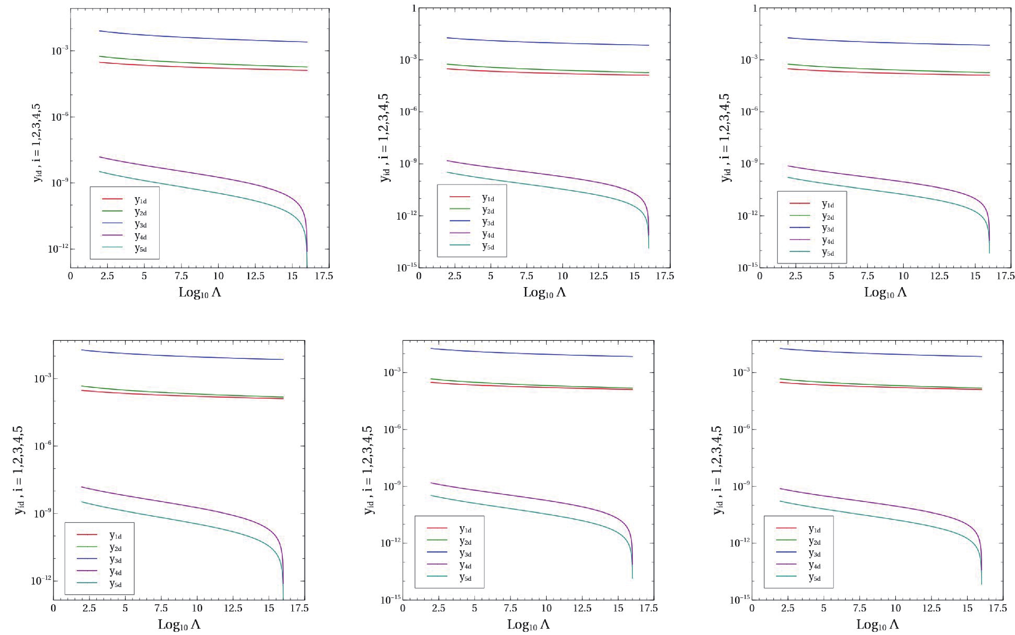
Figure 2. (color online) Upper panel :
$ y_{id} $ vs.$ {\rm{Log}}_{10}\Lambda $ plot for BP1 with three different initial values of$ y_{4u}, y_{5u} $ at$ 10^{16} $ GeV. Lower panel :$ y_{id} $ vs.$ {\rm{Log}}_{10}\Lambda $ plot for BP2 with three different initial values of$ y_{4u}, y_{5u} $ at$ 10^{16} $ GeV.As we lower the energy scale, because the RGEs are coupled mutually,
$ y_{4d}, y_{5d} $ can obtain a non-zero but still very small value, compatible with flavor physics constraints at the EW scale. The trend of the evolution of other Yukawa couplings are the same as in the bottom-up approach, i.e., the lower the energy scale, the higher the Yukawa couplings. Again, the RG evolution curves corresponding to BP1 and BP2 are not appreciably different owing to the reason explained above. -
We consider tree level FCNCs in the quark sector of the
$ S_3 $ HDM. The flavor-changing Yukawa couplings are constrained using perturbativity criteria as well as relevant flavor physics observables originating from meson-decays, meson-mixing, etc. in the up- and down-type quark sectors. It can be inferred that the constraints arising from meson mixing place more stringent bounds on the flavor-changing couplings compared to the others.Initially, we find a parameter space compatible with recent flavor physics data, spanned by several flavor-changing Yukawa couplings and mixing angles at the EW scale. Subsequently, we evolve the couplings from the EW scale via the bottom-up approach through coupled RGEs to analyze the high scale validity of the model. The trends of the evolution of all the Yukawa couplings are similar, i.e., the couplings decrease with increasing energy scale.
Finally, we start with zero values of
$ y_{4d}, y_{5d} $ at$ 10^{16} $ GeV as an artifact of some hidden symmetry and evolve them to the EW scale via reverse running. We end up with non-zero but negligible values of$ y_{4d}, y_{5d} $ generated radiatively at the EW scale, which are still compatible with all the flavor physics constraints. -
The one-loop beta RGEs of the Yukawa couplings are listed below.
$ \begin{aligned}[b]\\ 16 \pi^2 \frac{{\rm d} y_{1u}}{{\rm d}t} =& \frac{1}{2} (9 y_{1d}^2 y_{1u}-8 y_{1d} y_{2d} y_{2u}+4 y_{1l}^2 y_{1u}+15 y_{1u}^3+2 y_{1u} y_{2d}^2+6 y_{1u} y_{2u}^2+6 y_{1u} y_{3d}^2 \\& +2 y_{1u} y_{3l}^2+6 y_{1u} y_{3u}^2+2 y_{1u} y_{4u}^2+y_{1u} y_{5d}^2+y_{1u} y_{5u}^2-4 y_{3d} y_{4u} y_{5d}) + a_u y_{1u} \,, \\ 16 \pi^2 \frac{{\rm d} y_{2u}}{{\rm d}t} =& \frac{1}{2} (y_{1d}^2 y_{2u}-4 y_{1d} y_{1u} y_{2d}+3 y_{1u}^2 y_{2u}+14 y_{2d}^2 y_{2u}-4 y_{2d} y_{4d} y_{4u}+4 y_{2l}^2 y_{2u}+18 y_{2u}^3 \\& +6 y_{2u} y_{4d}^2 +2 y_{2u} y_{4l}^2+8 y_{2u} y_{4u}^2+3 y_{2u} y_{5d}^2+2 y_{2u} y_{5l}^2+7 y_{2u} y_{5u}^2) + a_u y_{2u}\,, \\ 16 \pi^2 \frac{{\rm d} y_{3u}}{{\rm d}t} =& 6 y_{1d}^2 y_{3u}-4 y_{1d} y_{4d} y_{5u}+\frac{1}{2} y_{3u} (4 y_{1l}^2+12 y_{1u}^2+3 y_{3d}^2+2 y_{3l}^2+9 y_{3u}^2 \\& +2 (y_{4d}^2+y_{4u}^2+2 y_{5u}^2)) + a_u y_{3u}\,, \\ 16 \pi^2 \frac{{\rm d} y_{_{4u}}}{{\rm d}t} =& y_{1u}^2 y_{4u}-2 y_{1u} y_{3d} y_{5d}+6 y_{2d}^2 y_{4u}-4 y_{2d} y_{2u} y_{4d}+\frac{1}{2} y_{4u} (4 y_{2l}^2+16 y_{2u}^2+y_{3d}^2+y_{3u}^2 \\ & +2 (2 y_{4d}^2+y_{4l}^2+5 y_{4u}^2+3 y_{5d}^2+y_{5l}^2+3 y_{5u}^2)) + a_u y_{4u} \,, \\ 16 \pi^2 \frac{{\rm d} y_{5u}}{{\rm d}t} = & \frac{1}{2} (y_{5u} (y_{1d}^2+y_{1u}^2+6 y_{2d}^2+4 y_{2l}^2+14 y_{2u}^2+2 y_{3u}^2+6 y_{4d}^2+2 y_{4l}^2+6 y_{4u}^2+3 y_{5d}^2+2 y_{5l}^2) \\& -4 y_{1d} y_{3u} y_{4d}+11 y_{5u}^3) + a_u y_{5u}\,, \end{aligned}$ 
$ \begin{aligned}[b] 16 \pi^2 \frac{{\rm d} y_{1d}}{{\rm d}t} = & \frac{1}{2} (15 y_{1d}^3+y_{1d} (4 y_{1l}^2+9 y_{1u}^2+6 y_{2d}^2+2 y_{2u}^2+6 y_{3d}^2+2 y_{3l}^2+6 y_{3u}^2+2 y_{4d}^2+y_{5d}^2+y_{5u}^2) \\ & -4 (2 y_{1u} y_{2d} y_{2u}+y_{3u} y_{4d} y_{5u})) + a_d y_{1d} \,, \\ 16 \pi^2 \frac{{\rm d} y_{2d}}{{\rm d}t} = & \frac{1}{2} (3 y_{1d}^2 y_{2d}-4 y_{1d} y_{1u} y_{2u}+y_{1u}^2 y_{2d}+18 y_{2d}^3+4 y_{2d} y_{2l}^2+14 y_{2d} y_{2u}^2+8 y_{2d} y_{4d}^2+2 y_{2d} y_{4l}^2 \\ & +6 y_{2d} y_{4u}^2+7 y_{2d} y_{5d}^2+2 y_{2d} y_{5l}^2+3 y_{2d} y_{5u}^2-4 y_{2u} y_{4d} y_{4u}) + a_d y_{2d}\,, \\ 16 \pi^2 \frac{{\rm d} y_{3d}}{{\rm d}t} = & 6 y_{1d}^2 y_{3d}+2 y_{1l}^2 y_{3d}+6 y_{1u}^2 y_{3d}-4 y_{1u} y_{4u} y_{5d}+\frac{9 y_{3d}^3}{2}+y_{3d} y_{3l}^2+\frac{3 y_{3d} y_{3u}^2}{2} \\& +y_{3d} y_{4d}^2+y_{3d} y_{4u}^2+2 y_{3d} y_{5d}^2 + a_d y_{3d} \,, \\ 16 \pi^2 \frac{{\rm d} y_{4d}}{{\rm d}t} =& y_{1d}^2 y_{4d}-2 y_{1d} y_{3u} y_{5u}+8 y_{2d}^2 y_{4d}-4 y_{2d} y_{2u} y_{4u}+\frac{1}{2} y_{4d} (4 y_{2l}^2+12 y_{2u}^2+y_{3d}^2+y_{3u}^2 \\& +2 (5 y_{4d}^2+y_{4l}^2+2 y_{4u}^2+3 y_{5d}^2+y_{5l}^2+3 y_{5u}^2)) + a_d y_{4d} \,, \\ 16 \pi^2 \frac{{\rm d} y_{5d}}{{\rm d}t} = & \frac{1}{2} (y_{5d} (y_{1d}^2+14 y_{2d}^2+4 y_{2l}^2+6 y_{2u}^2+2 y_{3d}^2+6 y_{4d}^2+2 y_{4l}^2+6 y_{4u}^2+11 y_{5d}^2+2 y_{5l}^2+3 y_{5u}^2) \\ & +y_{1u}^2 y_{5d}-4 y_{1u} y_{3d} y_{4u}) + a_d y_{5d} \,, \\ 16 \pi^2 \frac{{\rm d} y_{1l}}{{\rm d}t} = & \frac{1}{2} y_{1l} (12 y_{1d}^2 + 7 y_{1l}^2 + 2 (6 y_{1u}^2 + 3 y_{2l}^2 + 3 y_{3d}^2 + y_{3l}^2 + 3 y_{3u}^2 + y_{4l}^2) + y_{5l}^2) + a_l y_{1l}\,, \\ 16 \pi^2 \frac{{\rm d} y_{2l}}{{\rm d}t} = & \frac{1}{2} y_{2l} (3 y_{1l}^2 + 12 y_{2d}^2 + 10 y_{2l}^2 + 12 y_{2u}^2 + 6 y_{4d}^2 + 4 y_{4l}^2 + 6 y_{4u}^2 + 6 y_{5d}^2 + 3 y_{5l}^2 + 6 y_{5u}^2) + a_l y_{2l}\,, \\ 16 \pi^2 \frac{{\rm d} y_{3l}}{{\rm d}t} =& \frac{1}{2} y_{3l} (12 y_{1d}^2 + 4 y_{1l}^2 + 12 y_{1u}^2 + 6 y_{3d}^2 + 5 y_{3l}^2 + 6 y_{3u}^2 + 2 y_{4l}^2 + 4 y_{5l}^2) + a_l y_{3l}\,, \\ 16 \pi^2 \frac{{\rm d} y_{4l}}{{\rm d}t} = & \frac{1}{2} y_{4l} (2 y_{1l}^2 + 12 y_{2d}^2 + 8 y_{2l}^2 + 12 y_{2u}^2 + y{3l}^2 + 6 y_{4d}^2 + 6 y_{4l}^2 + 6 y_{4u}^2 + 6 y_{5d}^2 + 2 y_{5l}^2 + 6 y_{5u}^2) + a_l y_{4l}\,, \\ 16 \pi^2 \frac{{\rm d} y_{5l}}{{\rm d}t} = & \frac{1}{2} y_{5l} (y_{1l}^2 + 12 y_{2d}^2 + 6 y{2l}^2 + 12 y_{2u}^2 + 2 y_{3l}^2 + 6 y_{4d}^2 + 2 y_{4l}^2 + 6 y_{4u}^2 + 6 y_{5d}^2 + 7 y_{5l}^2 + 6 y_{5u}^2) + a_l y_{5l}\,. \end{aligned}\tag{A1}$

With
$ \begin{aligned}[b] a_d = - 8 g_s^2 - \frac{9}{4} g^2 - \frac{5}{12} g'^2 \,, \qquad\quad a_u = - 8 g_s^2 - \frac{9}{4} g^2 - \frac{17}{12} g'^2 \,,\qquad\quad a_l = - \frac{9}{4} g^2 - \frac{15}{4} g'^2 \,. \end{aligned}\tag{A2}$

-
Below, we show the interactions between the neutral
$C P$ -even scalars$ h, H_1, H_2 $ and the gauge bosons$ V = W^{\pm},Z $ .$ g_{hVV} = \big(O_{11}s_\beta c_\gamma + O_{21}s_\beta s_\gamma + O_{31} c_\beta\big) \frac{n M_V^2}{v}, \tag{B1a} $

$ g_{H_1VV} = \big(O_{12}s_\beta c_\gamma + O_{22}s_\beta s_\gamma + O_{32} c_\beta\big) \frac{n M_V^2}{v} , \tag{B1b}$

$ g_{H_2VV} = \big(O_{13}s_\beta c_\gamma + O_{23}s_\beta s_\gamma + O_{33} c_\beta\big) \frac{n M_V^2}{v} ,\tag{B1c} $

where
$ n = 2(1) $ for$ W^{\pm}(Z) $ .The flavor-conserving couplings of h with u-quarks are
$ y_{huu} = O_{31} y_{1u} - O_{21} s_\gamma y_{2u} - O_{11} c_\gamma y_{2u} , \tag{B2a}$

$ y_{hcc} = O_{31} y_{1u} + O_{21} s_\gamma y_{2u} + O_{11} c_\gamma y_{2u} , \tag{B2b}$

$ y_{htt} = \frac{O_{31}}{c_\beta} y_{3u} . \tag{B2c}$

The flavor-violating couplings with u-quarks are
$ y_{huc} = \frac{y_{2u}}{\sqrt{2}}\Big(-O_{21} c_\gamma + O_{11} s_\gamma\Big), \tag{B3a} $

$ y_{hut} = \frac{y_{5u}}{2}\Big(O_{21} \sqrt{1 + s_\gamma} - O_{11} \sqrt{1 - s_\gamma}), \tag{B3b} $

$ y_{hct} = \frac{y_{5u}}{2}\Big(O_{21} \sqrt{1 - s_\gamma} + O_{11} \sqrt{1 + s_\gamma}), \tag{B3c} $

$ y_{H_1uc} = \frac{y_{2u}}{\sqrt{2}}\Big(-O_{22} c_\gamma + O_{12} s_\gamma\Big), \tag{B3d} $

$ y_{H_1ut} = \frac{y_{5u}}{2}\Big(O_{22} \sqrt{1 + s_\gamma} - O_{12} \sqrt{1 - s_\gamma}),\tag{B3e} $

$ y_{H_1ct} = \frac{y_{5u}}{2}\Big(O_{22} \sqrt{1 - s_\gamma} + O_{12} \sqrt{1 + s_\gamma}), \tag{B3f}$

$ y_{H_2uc} = \frac{y_{2u}}{\sqrt{2}}\Big(-O_{23} c_\gamma + O_{13} s_\gamma\Big), \tag{B3g} $

$ y_{H_2ut} = \frac{y_{5u}}{2}\Big(O_{23} \sqrt{1 + s_\gamma} - O_{13} \sqrt{1 - s_\gamma}), \tag{B3h}$

$ y_{H_2ct} = \frac{y_{5u}}{2}\Big(O_{23} \sqrt{1 - s_\gamma} + O_{13} \sqrt{1 + s_\gamma}). \tag{B3i} $

The corresponding couplings for the down-sector can be obtained via the substitutions
$ u \rightarrow d $ ,$ c \rightarrow s $ , and$ t \rightarrow b $ .It is noted that the flavor-violating couplings of
$ A_1 $ ($ A_2 $ ) are the same as the corresponding couplings of$ H_1 $ ($ H_2 $ ).
Flavor-alignment in an S3-symmetric Higgs sector and its RG-behavior
- Received Date: 2022-03-31
- Available Online: 2022-12-15
Abstract: A three Higgs-doublet model exhibiting


 DownLoad: